西电数字信号处理大作业
西安电子科技大学数字信号处理上机作业

数字信号处理MATLAB上机作业M 2.21.题目The square wave and the sawtooth wave are two periodic sequences as sketched in figure ing the function stem. The input data specified by the user are: desired length L of the sequence, peak value A, and the period N. For the square wave sequence an additional user-specified parameter is the duty cycle, which is the percent of the period for which the signal is positive. Using this program generate the first 100 samples of each of the above sequences with a sampling rate of 20 kHz ,a peak value of 7, a period of 13 ,and a duty cycle of 60% for the square wave.2.程序% 用户定义各项参数参数A = input('The peak value =');L = input('Length of sequence =');N = input('The period of sequence =');FT = input('The desired sampling frequency =');DC = input('The square wave duty cycle = ');% 产生所需要的信号t = 0:L-1;T = 1/FT;x = A*sawtooth(2*pi*t/N);y = A*square(2*pi*(t/N),DC);% Plotsubplot(2,1,1)stem(t,x);ylabel('幅度');xlabel('n');subplot(2,1,2)stem(t,y);ylabel('幅度');xlabel('n');3.结果4.结果分析M 2.41.题目(a)Write a matlab program to generate a sinusoidal sequence x[n]= Acos(ω0 n+Ф) and plot thesequence using the stem function. The input data specified by the user are the desired length L, amplitude A, the angular frequency ω0 , and the phase Фwhere 0<ω0 <pi and 0<=Ф<=2pi. Using this program generate the sinusoidal sequences shown in figure 2.15. (b)Generate sinusoidal sequences with the angular frequencies given in Problem 2.22.Determine the period of each sequence from the plot and verify the result theoretically. 2.程序%用户定义的参数L = input('Desired length = ');A = input('Amplitude = ');omega = input('Angular frequency = ');phi = input('Phase = ');%信号产生n = 0:L-1;x = A*cos(omega*n + phi);stem(n,x);xlabel('n');ylabel('幅度');title(['\omega_{o} = ',num2str(omega)]);3.结果(a)ω0=0ω0=0.1πω0=0.8πω0=1.2π(b)ω0=0.14πω0=0.24πω0=0.34πω0=0.68πω0=0.75π4.结果分析M 2.51.题目Generate the sequences of problem 2.21(b) to 2.21(e) using matlab.2.程序(b)n = 0 : 99;x=sin(0.6*pi*n+0.6*pi);stem(n,x);xlabel('n');ylabel('幅度');(c)n = 0 : 99;x=2*cos(1.1*pi*n-0.5*pi)+2*sin(0.7*pi*n);stem(n,x);xlabel('n');ylabel('幅度');(d)n = 0 : 99;x=3*sin(1.3*pi*n-4*cos(0.3*pi*n+0.45*pi));stem(n,x);xlabel('n');ylabel('幅度');(e)n = 0 : 99;x=5*sin(1.2*pi*n+0.65*pi)+4*sin(0.8*pi*n)-cos(0.8*pi*n);stem(n,x);xlabel('n');ylabel('幅度');(f)n = 0 : 99;x=mod(n,6);stem(n,x);xlabel('n');ylabel('幅度');3.结果(b)(c)(d)(e)(f)4.结果分析M 2.61.题目Write a matlab program to plot a continuous-time sinusoidal signal and its sampled version and verify figure 2.19. You need to use the hold function to keep both plots.2.程序%用户定义的参数fo = input('Frequency of sinusoid in Hz = ');FT = input('Samplig frequency in Hz = ');%产生信号t = 0:0.001:1;g1 = cos(2*pi*fo*t);plot(t,g1,'-')xlabel('时间t');ylabel('幅度')holdn = 0:1:FT;gs = cos(2*pi*fo*n/FT);plot(n/FT,gs,'o');hold off3.结果4.结果分析M 3.11.题目Using program 3_1 determine and plot the real and imaginary parts and the magnitude and phase spectra of the following DTFT for various values of r and θ:G(e jω)=1, 0<r<1.1−2r(cosθ)e−jω+r2e−2jω2.程序%program 3_1%discrete-time fourier transform computatition%k=input('Number of frequency points = ');num=input('Numerator coefficients= ');den=input('Denominator coefficients= ');%computer the frequency responsew=0:pi/k:pi;h=freqz(num,den,w);%plot the frequency responsesubplot(221)plot(w/pi,real(h));gridtitle('real part')xlabel('\omega/\pi');ylabel('Amplitude') subplot(222)plot(w/pi,imag(h));gridtitle('imaginary part')xlabel('\omega/\pi');ylabel('Amplitude') subplot(223)plot(w/pi,abs(h));gridtitle('magnitude spectrum')xlabel('\omega/\pi');ylabel('magnitude') subplot(224)plot(w/pi,angle(h));gridtitle('phase spectrum')xlabel('\omega/\pi');ylabel('phase,radians')3.结果(a)r=0.8 θ=π/6(b)r=0.6 θ=π/34.结果分析M 3.41.题目Using matlab verify the following general properties of the DTFT as listed in Table 3.2:(a) Linearity, (b) time-shifting, (c) frequency-shifting, (d) differentiation-in-frequency, (e) convolution, (f) modulation, and (g) Parseval’s relation. Since all data in matlab have to be finite-length vectors, the sequences to be used to verify the properties are thus restricted to be of finite length.2.程序%先定义两个信号N = input('The length of the sequence = ');k = 0:N-1;%g为正弦信号g = 2*sin(2*pi*k/(N/2));%h为余弦信号h = 3*cos(2*pi*k/(N/2));[G,w] = freqz(g,1);[H,w] = freqz(h,1);%*************************************************************************%% 线性性质alpha = 0.5;beta = 0.25;y = alpha*g+beta*h;[Y,w] = freqz(y,1);figure(1);subplot(211),plot(w/pi,abs(Y));xlabel('\omega/\pi');ylabel('|Y(e^j^\omega)|');title('线性叠加后的频率特性');grid;% 画出Y 的频率特性subplot(212),plot(w/pi,alpha*abs(G)+beta*abs(H));xlabel('\omega/\pi');ylabel('\alpha|G(e^j^\omega)|+\beta|H(e^j^\omega)|');title('线性叠加前的频率特性');grid;% 画出alpha*G+beta*H 的频率特性%*************************************************************************% % 时移性质n0 = 10;%时移10个的单位y2 = [zeros([1,n0]) g];[Y2,w] = freqz(y2,1);G0 = exp(-j*w*n0).*G;figure(2);subplot(211),plot(w/pi,abs(G0));xlabel('\omega/\pi');ylabel('|G0(e^j^\omega)|');title('G0的频率特性');grid;% 画出G0的频率特性subplot(212),plot(w/pi,abs(Y2));xlabel('\omega/\pi');ylabel('|Y2(e^j^\omega)|');title('Y2的频率特性');grid;% 画出Y2 的频率特性%*************************************************************************% % 频移特性w0 = pi/2; % 频移pi/2r=256; %the value of w0 in terms of number of samplesk = 0:N-1;y3 = g.*exp(j*w0*k);[Y3,w] = freqz(y3,1);% 对采样的512个点分别进行减少pi/2,从而生成G(exp(w-w0))k = 0:511;w = -w0+pi*k/512;G1 = freqz(g,1,w);figure(3);subplot(211),plot(w/pi,abs(Y3));xlabel('\omega/\pi');ylabel('|Y3(e^j^\omega)|');title('Y3的频率特性');grid;% 画出Y3的频率特性subplot(212),plot(w/pi,abs(G1));xlabel('\omega/\pi');ylabel('|G1(e^j^\omega)|');title('G1的频率特性');grid;% 画出G1 的频率特性%*************************************************************************% % 频域微分k = 0:N-1;y4 = k.*g;[Y4,w] = freqz(y4,1);%在频域进行微分y0 = ((-1).^k).*g;G2 = [G(2:512)' sum(y0)]';delG = (G2-G)*512/pi;figure(4);subplot(211),plot(w/pi,abs(Y4));xlabel('\omega/\pi');ylabel('|Y4(e^j^\omega)|');title('Y4的频率特性');grid;% 画出Y4的频率特性subplot(212),plot(w/pi,abs(delG));xlabel('\omega/\pi');ylabel('|delG(e^j^\omega)|');title('delG的频率特性');grid;% 画出delG的频率特性%*************************************************************************% % 相乘性质y5 = conv(g,h);%时域卷积[Y5,w] = freqz(y5,1);figure(5);subplot(211),plot(w/pi,abs(Y5));xlabel('\omega/\pi');ylabel('|Y5(e^j^\omega)|');title('Y5的频率特性');grid;% 画出Y5的频率特性subplot(212),plot(w/pi,abs(G.*H));%频域乘积xlabel('\omega/\pi');ylabel('|G.*H(e^j^\omega)|');title('G.*H的频率特性');grid;% 画出G.*H的频率特性%*************************************************************************% % 帕斯瓦尔定理y6 = g.*h;%对于freqz函数,在0到2pi直接取样[Y6,w] = freqz(y6,1,512,'whole');[G0,w] = freqz(g,1,512,'whole');[H0,w] = freqz(h,1,512,'whole');% Evaluate the sample value at w = pi/2% and verify with Y6 at pi/2H1 = [fliplr(H0(1:129)') fliplr(H0(130:512)')]';val = 1/(512)*sum(G0.*H1);% Compare val with Y6(129) i.e sample at pi/2 % Can extend this to other points similarly% Parsevals theoremval1 = sum(g.*conj(h));val2 = sum(G0.*conj(H0))/512;% Comapre val1 with val23.结果(a)(b)(c)(d)(e)4.结果分析M 3.81.题目Using matlab compute the N-point DFTs of the length-N sequences of Problem 3.12 for N=3, 5, 7, and 10. Compare your results with that obtained by evaluating the DTFTs computed in Problem 3.12 at ω= 2pik/N, k=0, 1,……N-1.2.程序%用户定义N的长度N = input('The value of N = ');k = -N:N;y1 = ones([1,2*N+1]);w = 0:2*pi/255:2*pi;Y1 = freqz(y1, 1, w);%对y1做傅里叶变换Y1dft = fft(y1);k = 0:1:2*N;plot(w/pi,abs(Y1),k*2/(2*N+1),abs(Y1dft),'o');grid;xlabel('归一化频率');ylabel('幅度');(a)clf;N = input('The value of N = ');k = -N:N;y1 = ones([1,2*N+1]);w = 0:2*pi/255:2*pi;Y1 = freqz(y1, 1, w);Y1dft = fft(y1);k = 0:1:2*N;plot(w/pi,abs(Y1),k*2/(2*N+1),abs(Y1dft),'o');xlabel('Normalized frequency');ylabel('Amplitude');(b)%用户定义N的长度N = input('The value of N = ');k = -N:N;y1 = ones([1,2*N+1]);y2 = y1 - abs(k)/N;w = 0:2*pi/255:2*pi;Y2 = freqz(y2, 1, w);%对y1做傅里叶变换Y2dft = fft(y2);k = 0:1:2*N;plot(w/pi,abs(Y2),k*2/(2*N+1),abs(Y2dft),'o');grid;xlabel('归一化频率');ylabel('幅度');(c)%用户定义N的长度N = input('The value of N = ');k = -N:N;y3 =cos(pi*k/(2*N));w = 0:2*pi/255:2*pi;Y3 = freqz(y3, 1, w);%对y1做傅里叶变换Y3dft = fft(y3);k = 0:1:2*N;plot(w/pi,abs(Y3),k*2/(2*N+1),abs(Y3dft),'o');grid;xlabel('归一化频率');ylabel('幅度');3.结果(a)N=3N=5 N=7N=10 (b)N=3N=5 N=7N=10 (c)N=3N=5 N=7N=104.结果分析M 3.191.题目Using Program 3_10 determine the z-transform as a ratio of two polynomials in z-1 from each of the partial-fraction expansions listed below:(a)X1(z)=−2+104+z−1−82+z−1,|z|>0.5,(b)X2(z)=3.5−21−0.5z−1−3+z−11−0.25z−2,|z|>0.5,(c)X3(z)=5(3+2z−1)2−43+2z−1+31+0.81z−2,|z|>0.9,(d)X4(z)=4+105+2z−1+z−16+5z−1+z−2,|z|>0.5.2.程序% Program 3_10% Partical-Fraction Expansion to rational z-Transform %r = input('Type in the residues = ');p = input('Type in the poles = ');k = input('Type in the constants = ');[num, den] = residuez(r,p,k);disp('Numberator polynominal coefficients');disp(num) disp('Denominator polynomial coefficients'); disp(den)4.结果分析M 4.61.题目Plot the magnitude and phase responses of the causal IIR digital transfer functionH(z)=0.0534(1+z−1)(1−1.0166z−1+z−2) (1−0.683z−1)(1−1.4461z−1+0.7957z−2).What type of filter does this transfer function represent? Determine the difference equation representation of the above transfer function.2.程序b=[0.0534 -0.00088644 -0.00088644 0.0534];a=[1 -2.1291 1.7833863 -0.5434631];figure(1)freqz(b,a);figure(2)[H,w]=freqz(b,a);plot(w/pi,abs(H)),grid;xlabel('Normalized Frequency (\times\pi rad/sample)'),ylabel('Magnitude');幅度化成真值之后:4.结果分析H(z)=0.0534−0.00088644z−1−0.00088644z−2+0.0534z−31−2.1291z−1+1.7833863z−2−0.5434631z−3M 4.71.题目Plot the magnitude and phase responses of the causal IIR digital transfer functionH(z)=(1−z−1)4(1−1.499z−1+0.8482z−2)(1−1.5548z−1+0.6493z−2).2.程序b=[1 -4 6 -4 1];a=[1 -3.0538 3.8227 -2.2837 0.5472]; figure(1)freqz(b,a);figure(2)[H,w]=freqz(b,a);plot(w/pi,abs(H)),grid;xlabel('Normalized Frequency (\times\pi rad/sample)'), ylabel('Magnitude');3.结果4.结果分析。
西电信号大作业(歌曲人声消除)

信号与系统课程实践报告1内容与要求通过信号分析的方法设计一个软件或者一个仿真程序,程序的主要功能是完成对歌曲中演唱者语音的消除。
试分析软件的根本设计思路、根本原理,并通过MA TLAB程序设计语言完成设计。
更进一步地,从理论和实用的角度改善软件性能的方法和措施。
2 思路与方案歌曲的伴奏左右声道相同,人声不同。
所以通过左右声道不同处理信号,然后通过频率分析做带阻滤波滤除主要人声信号。
3 成果及展示代码:clear;clc;[X,fs]=audioread('D:\文本文档\林.wav');ts=1/fs;N=length(X)-1;t=0:1/fs:N/fs;Nfft=N;df=fs/Nfft;fk=(-Nfft/2:Nfft/2-1)*df;a1=1;a2=-1;b1=1;b2=-1;%别离左声道和右声道SoundLeft=X(:,1);SoundRight=X(:,2);%对左声道和右声道进行快速傅里叶变换SoundLeft_f=ts*fftshift(fft(SoundLeft,N));SoundRight_f=ts*fftshift(fft(SoundRight,N));%显示左右声道幅度变化figure(1)subplot(411)plot(t,SoundLeft);subplot(412)plot(t,SoundRight);%显示左右声道频率变化subplot(413)f_range=[-5000,5000,0,0.1];plot(fk,SoundLeft_f);axis(f_range);subplot(414)plot(fk,SoundRight_f);axis(f_range);NewLeft=a1*SoundLeft+a2*SoundRight; NewRight=b1*SoundLeft+b2*SoundRight; Sound(:,1)=NewLeft;Sound(:,2)=NewRight;Sound_Left_f=ts*fftshift(fft(NewLeft,N)); Sound_Right_f=ts*fftshift(fft(NewRight,N)); figure(2)subplot(411)plot(t,NewLeft);subplot(412)plot(t,NewRight);f_range=[-5000,5000,0,0.1];subplot(413)plot(fk,Sound_Left_f);axis(f_range);subplot(414)plot(fk,Sound_Right_f);axis(f_range);BP=fir1(300,[800,2200]/(fs/2));%根据左右声道差异进行滤波【800,2200】Hz CutDown=filter(BP,1,Sound);Sound_Final=Sound-0.6*abs(CutDown);Sound_Final_f=ts*fftshift(fft(Sound_Final,N));figure(3)subplot(211)plot(t,Sound_Final);subplot(212)f_range=[-5000,5000,0,0.1];plot(fk,Sound_Final_f);axis(f_range);audiowrite('D:\文本文档\林_去人声.wav',Sound_Final,fs);1歌曲原始左右声道的幅度和频率曲线2相减得到的信号幅度和频率曲线3进行消除人声处理后信号的幅度和频率曲线4 总结与感想在本次实践中,熟悉了matlab的操作,了解了很多命令。
西电DSP大作业任务报告
DSP实验课程序设计报告学院:电子工程学院学号:1202121013姓名:赵海霞指导教师:苏涛DSP实验课大作业设计一实验目的在DSP上实现线性调频信号的脉冲压缩、动目标显示(MTI)和动目标检测(MTD),并将结果与MATLAB上的结果进行误差仿真。
二实验内容2.1 MATLAB仿真设定带宽、脉宽、采样率、脉冲重复频率,用MATLAB产生16个脉冲的LFM,每个脉冲有4个目标(静止,低速,高速),依次做2.1.1 脉压2.1.2 相邻2脉冲做MTI,产生15个脉冲2.1.3 16个脉冲到齐后,做MTD,输出16个多普勒通道2.2 DSP实现将MATLAB产生的信号,在visual dsp中做脉压,MTI、MTD,并将结果与MATLAB作比较。
三实验原理3.1 线性调频线性调频脉冲压缩体制的发射信号其载频在脉冲宽度内按线性规律变化即用对载频进行调制(线性调频)的方法展宽发射信号的频谱,在大时宽的前提下扩展了信号的带宽。
若线性调频信号中心频率为f,脉宽为τ,带宽为B,幅度为A,μ为调频斜率,则其表达式如下:]212cos[)()(20t t f t rect A t x μπτ+••=;)(为矩形函数rect 在相参雷达中,线性调频信号可以用复数形式表示,即)]212(exp[)()(20t t f j t rect A t x μπτ+••= 在脉冲宽度内,信号的角频率由220μτπ-f 变化到220μτπ+f 。
3.2 脉冲压缩原理脉冲雷达信号发射时,脉冲宽度τ决定着雷达的发射能量,发射能量越大, 作用距离越远;在传统的脉冲雷达信号中,脉冲宽度同时还决定着信号的频率宽度B ,即带宽与时宽是一种近似倒数的关系。
脉冲越宽,频域带宽越窄,距离分辨率越低。
脉冲压缩的主要目的是为了解决信号的作用距离和信号的距离分辨率之间的矛盾。
为了提高信号的作用距离,我们就需要提高信号的发射功率,因此,必须提高发射信号的脉冲宽度,而为了提高信号的距离分辨率,又要求降低信号的脉冲宽度。
西安电子科大数字信号处理课后实验答案

一系统响应及稳定性的实验报告一. 实验目的:(1)掌握 求系统响应的方法。
(2)掌握时域离散系统的时域特性。
(3)分析、观察及检验系统的稳定性。
二. 实验原理与方法:1.在时域中,描写系统特性的方法是差分方程和单位脉冲响应,在频域可以用系统函数描述系统特性。
已知输入信号可以由差分方程、单位脉冲响应或系统函数求出系统对于该输入信号的响应。
在计算机上可用filter 函数求差分方程的解, conv 函数计算输入信号和系统的单位脉冲响应的线性卷积,求出系统的响应。
2.系统的时域特性指的是系统的线性时不变性质、因果性和稳定性。
3.系统的稳定性是指对任意有界的输入信号,系统都能得到有界的系统响应。
或者系统的单位脉冲响应满足绝对可和的条件。
系统的稳定性由其差分方程的系数决定。
实际中检查系统是否稳定,不可能检查系统对所有有界的输入信号,输出是否都是有界输出,或者检查系统的单位脉冲响应满足绝对可和的条件。
可行的方法是在系统的输入端加入单位阶跃序列,如果系统的输出趋近一个常数(包括零),就可以断定系统是稳定的[19]。
系统的稳态输出是指当∞→n 时,系统的输出。
如果系统稳定,信号加入系统后,系统输出的开始一段称为暂态效应,随n 的加大,幅度趋于稳定,达到稳态输出。
三.实验内容及步骤:1.编制程序,包括产生输入信号、单位脉冲响应序列的子程序,用filter 函数或conv 函数求解系统输出响应的主程序。
程序中要有绘制信号波形的功能。
2.给定一个低通滤波器的差分方程为)1(9.0)1(05.0)(05.0)(-+-+=n y n x n x n y a) 分别求出系统对)()(81n R n x =和)()(2n u n x =的响应序列,并画出其波形。
b) 求出系统的单位冲响应,画出其波形。
3.给定系统的单位脉冲响应为)()(101n R n h =)3()2(5.2)1(5.2)()(2-+-+-+=n n n n n h δδδδ 用线性卷积法分别求系统h 1(n)和h 2(n)对)()(81n R n x =的输出响应,并画出波形。
西电数字信号处理大作业
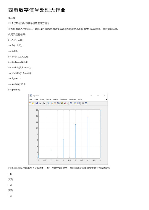
西电数字信号处理⼤作业第⼆章2.25 已知线性时不变系统的差分⽅程为若系统的输⼊序列x(x)={1,2,3,4,2,1}编写利⽤递推法计算系统零状态响应的MATLAB程序,并计算出结果。
代码及运⾏结果:>> A=[1,-0.5];>> B=[1,0,2];>> n=0:5;>> xn=[1,2,3,4,2,1];>> zx=[0,0,0];zy=0;>> zi=filtic(B,A,zy,zx);>> yn=filter(B,A,xn,zi);>> figure(1)>> stem(n,yn,'.');>> grid on;2.28图所⽰系统是由四个⼦系统T1、T2、T3和T4组成的,分别⽤单位脉冲响应或差分⽅程描述为T1:其他T2:其他T3:T4:编写计算整个系统的单位脉冲响应h(n),0≤n≤99的MATLAB程序,并计算结果。
代码及结果如下:>> a=0.25;b=0.5;c=0.25;>> ys=0;>> xn=[1,zeros(1,99)];>> B=[a,b,c];>> A=1;>> xi=filtic(B,A,ys);>> yn1=filter(B,A,xn,xi);>> h1=[1,1/2,1/4,1/8,1/16,1/32]; >> h2=[1,1,1,1,1,1];>> h3=conv(h1,h2);>> h31=[h3,zeros(1,89)]; >> yn2=yn1+h31;>> D=[1,1];C=[1,-0.9,0.81]; >> xi2=filtic(D,C,yn2,xi); >> xi2=filtic(D,C,ys);>> yn=filter(D,C,yn2,xi); >> n=0:99;>> figure(1)>> stem(n,yn,'.');>> title('单位脉冲响应'); >> xlabel('n');ylabel('yn');2.30 利⽤MATLAB画出受⾼斯噪声⼲扰的正弦信号的波形,表⽰为其中v(n)是均值为零、⽅差为1的⾼斯噪声。
西安电子科技大学-数字信号处理-试卷C答案
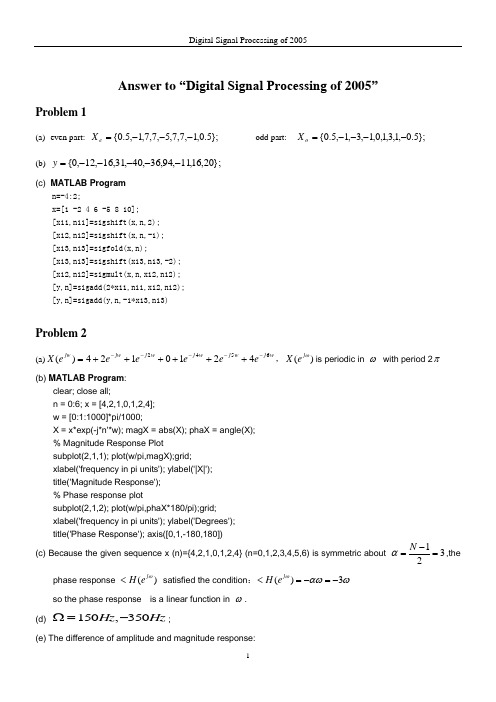
Answer to “Digital Signal Processing of 2005”Problem 1(a) even part: };5.0,1,7,7,5,7,7,1,5.0{---=e X odd part: };5.0,1,3,1,0,1,3,1,5.0{----=o X(b) };20,16,11,94,36,40,31,16,12,0{-----=y (c) MATLAB Programn=-4:2;x=[1 -2 4 6 -5 8 10]; [x11,n11]=sigshift(x,n,2); [x12,n12]=sigshift(x,n,-1); [x13,n13]=sigfold(x,n); [x13,n13]=sigshift(x13,n13,-2); [x12,n12]=sigmult(x,n,x12,n12); [y,n]=sigadd(2*x11,n11,x12,n12); [y,n]=sigadd(y,n,-1*x13,n13)Problem 2(a)w j w j w j w j jw jw e e e e e e X 65424210124)(-----++++++=,()j X e ωis periodic in ω with period 2π(b) MATLAB Program :clear; close all;n = 0:6; x = [4,2,1,0,1,2,4]; w = [0:1:1000]*pi/1000;X = x*exp(-j*n'*w); magX = abs(X); phaX = angle(X); % Magnitude Response Plotsubplot(2,1,1); plot(w/pi,magX);grid;xlabel('frequency in pi units'); ylabel('|X|'); title('Magnitude Response'); % Phase response plotsubplot(2,1,2); plot(w/pi,phaX*180/pi);grid;xlabel('frequency in pi units'); ylabel('Degrees'); title('Phase Response'); axis([0,1,-180,180])(c) Because the given sequence x (n)={4,2,1,0,1,2,4} (n=0,1,2,3,4,5,6) is symmetric about 132N α-==,the phase response ()j H e ω< satisfied the condition :()3j H e ωαωω<=-=- so the phase response is a linear function in ω.(d) 150,350Hz Hz Ω=-;(e) The difference of amplitude and magnitude response:Firstly, the amplitude response is a real function, and it may be both positive and negative. The magnitude response is always positive.Secondly, the phase response associated with the magnitude response is a discontinuous function. While the associated with the amplitude is a continuous linear function.Problem 3(a) )9.09.01/()1()(211------=z z z z HZero:0 and 1; Pole:-0.6 and 1.5; (b)1116151()212110.61 1.5H z z z--=⨯+⨯+-, 165()((0.6)(1.5))()2121n nh n u n =-+ (c) ROC : 0.6 1.5Z <<,()()()163531215212n nh n u n u n ⎛⎫⎛⎫=⨯--⨯--- ⎪ ⎪⎝⎭⎝⎭ Problem 4(a) y(n)={50,44,34,52};(b) y(n)={5,16,34,52,45,28,0}; (c) N=6;(d) MATLAB Program :Function y=circonv(x1,x2,N) If (length(x1)>N)error(“N must not be smaller than the length of sequence ”) elsex1=[x1,zeros(1,N-length(x1))]; endif(length(x2)>N)error(“N must not be smaller than the length of sequence ”)elsex2=[x2,zeros(1,N-length(x2))]; endy1=dft(x1,N).*dft(x2,N); y=idft(y,N);(e) DTFT is discrete in time domain, but continuous in frequency domain. The DFT is discrete both in time and frequency domain.The FFT is a very efficient method for calculating DFT.Problem 5(a) Direct form II uses the little delay and it can decrease the space of the compute. (b)The advantage of the linear-phase form:1. For frequency-selective filters, linear-phase structure is generally desirable to have a phase-responsethat is a linear function of frequency.2. This structure requires 50% fewer multiplications than the direct form. (c) Block diagrams are shown as under:1z -1z -1z -1z -1z -1z -()x n )n()x n1-1-Problem 6(a) we use Hamming or Blackman window to design the bandpass filter because it can provide us attenuationexceed 60dB .(b) According to Blackman window :first, Determine transition width =p s W W - ;second, Determine the type of the window according to s A ;third, Compute M using the formula MW W p s π2=- ; fourth, Compute ideal LPF2sp W W Wc +=;fifth, design the window needed, multiply point by point; sixth, determines p A R ,(c) MATLAB Program :%% Specifications about Blackman window: ws1 = 0.2*pi; % lower stopband edge wp1 = 0.3*pi; % lower passband edge wp2 = 0.6*pi; % upper passband edge ws2 = 0.7*pi; % upper stopband edge Rp = 0.5; % passband ripple As = 60; % stopband attenuation %tr_width = min((wp1-ws1),(ws2-wp2));M = ceil(6.6*pi/tr_width); M = 2*floor(M/2)+1, % choose odd M n = 0:M-1;w_ham = (hamming(M))';wc1 = (ws1+wp1)/2; wc2 = (ws2+wp2)/2; hd = ideal_lp(wc2,M)-ideal_lp(wc1,M); h = hd .* w_ham;[db,mag,pha,grd,w] = freqz_m(h,1); delta_w = pi/500;Asd = floor(-max(db([1:floor(ws1/delta_w)+1]))), % Actual AttnRpd = -min(db(ceil(wp1/delta_w)+1:floor(wp2/delta_w)+1)), % Actual passband ripple (5) %%% Filter Response Plotssubplot(2,2,1); stem(n,hd); title('Ideal Impulse Response: Bandpass'); axis([-1,M,min(hd)-0.1,max(hd)+0.1]); xlabel('n'); ylabel('hd(n)') set(gca,'XTickMode','manual','XTick',[0;M-1],'fontsize',10) subplot(2,2,2); stem(n,w_ham); title('Hamming Window'); axis([-1,M,-0.1,1.1]); xlabel('n'); ylabel('w_ham(n)')set(gca,'XTickMode','manual','XTick',[0;M-1],'fontsize',10) set(gca,'YTickMode','manual','YTick',[0;1],'fontsize',10)subplot(2,2,3); stem(n,h); title('Actual Impulse Response: Bandpass'); axis([-1,M,min(hd)-0.1,max(hd)+0.1]); xlabel('n'); ylabel('h(n)') set(gca,'XTickMode','manual','XTick',[0;M-1],'fontsize',10)subplot(2,2,4); plot(w/pi,db); title('Magnitude Response in dB');axis([0,1,-As-30,5]); xlabel('frequency in pi units'); ylabel('Decibels') set(gca,'XTickMode','manual','XTick',[0;0.3;0.4;0.5;0.6;1])set(gca,'XTickLabelMode','manual','XTickLabels',['0';'0.3';'0.4';'0.5';'0.6';'1'],... 'fontsize',10)set(gca,'TickMode','manual','YTick',[-50;0])set(gca,'YTickLabelMode','manual','YTickLabels',['-50';'0']);gridProblem 7Firstly, we use the given specifications ofs p s p A R ,,,ωω to design an analog lowpass IIR filter.Secondly, we change the analog lowpass IIR filter into the analog highpass IIR filter. Thirdly, we change the analog highpass IIR filter into the digital highpass IIR filter.。
数字信号处理实验报告(西电)
数字信号处理实验报告班级:****姓名:郭**学号:*****联系方式:*****西安电子科技大学电子工程学院绪论数字信号处理起源于十八世纪的数学,随着信息科学和计算机技术的迅速发展,数字信号处理的理论与应用得到迅速发展,形成一门极其重要的学科。
当今数字信号处理的理论和方法已经得到长足的发展,成为数字化时代的重要支撑,其在各个学科和技术领域中的应用具有悠久的历史,已经渗透到我们生活和工作的各个方面。
数字信号处理相对于模拟信号处理具有许多优点,比如灵活性好,数字信号处理系统的性能取决于系统参数,这些参数很容易修改,并且数字系统可以分时复用,用一套数字系统可以分是处理多路信号;高精度和高稳定性,数字系统的运算字符有足够高的精度,同时数字系统不会随使用环境的变化而变化,尤其使用了超大规模集成的DSP 芯片,简化了设备,更提高了系统稳定性和可靠性;便于开发和升级,由于软件可以方便传送,复制和升级,系统的性能可以得到不断地改善;功能强,数字信号处理不仅能够完成一维信号的处理,还可以试下安多维信号的处理;便于大规模集成,数字部件具有高度的规范性,对电路参数要求不严格,容易大规模集成和生产。
数字信号处理用途广泛,对其进行一系列学习与研究也是非常必要的。
本次通过对几个典型的数字信号实例分析来进一步学习和验证数字信号理论基础。
实验一主要是产生常见的信号序列和对数字信号进行简单处理,如三点滑动平均算法、调幅广播(AM )调制高频正弦信号和线性卷积。
实验二则是通过编程算法来了解DFT 的运算原理以及了解快速傅里叶变换FFT 的方法。
实验三是应用IRR 和FIR 滤波器对实际音频信号进行处理。
实验一●实验目的加深对序列基本知识的掌握理解●实验原理与方法1.几种常见的典型序列:0()1,00,0(){()()(),()sin()j n n n n u n x n Aex n a u n a x n A n σωωϕ+≥<====+单位阶跃序列:复指数序列:实指数序列:为实数 正弦序列:2.序列运算的应用:数字信号处理中经常需要将被加性噪声污染的信号中移除噪声,假定信号 s(n)被噪声d(n)所污染,得到了一个含噪声的信号()()()x n s n d n =+。
(1077)数字信号处理大作业1
h=fft(x,1024);%做1024点的快速傅里叶变换,满足频域抽样定理
ff=1000*(0:511)/1024;%将数字频率转换为模拟频率,单位为Hz
plot(ff,abs(h(1:512)));%显示信号的幅度谱,由于对称性,只显示一半
答:
\
西南大学网络与继续教育学院课程考试答题卷
2016年6月
课程名称【编号】:数字信号处理【1077】类别:网教专升本
专业:电气工程及其自动化
(横线以下为答题区)
答题不需复制题目,写明题目编号,按题目顺序答题
一、简答题。
1.答:
二、计算题。
1.答:
三、编程题。
1.答:t= -1:0.01:1;%以0.01秒周期进行抽样,并加矩形窗截断,满足抽样定理
- 1、下载文档前请自行甄别文档内容的完整性,平台不提供额外的编辑、内容补充、找答案等附加服务。
- 2、"仅部分预览"的文档,不可在线预览部分如存在完整性等问题,可反馈申请退款(可完整预览的文档不适用该条件!)。
- 3、如文档侵犯您的权益,请联系客服反馈,我们会尽快为您处理(人工客服工作时间:9:00-18:30)。
第二章2.25 已知线性时不变系统的差分方程为y(n)=−12y(n−1)+x(n)+2x(n−2)若系统的输入序列x(x)={1,2,3,4,2,1}编写利用递推法计算系统零状态响应的MATLAB程序,并计算出结果。
代码及运行结果:>> A=[1,-0.5];>> B=[1,0,2];>> n=0:5;>> xn=[1,2,3,4,2,1];>> zx=[0,0,0];zy=0;>> zi=filtic(B,A,zy,zx);>> yn=filter(B,A,xn,zi);>> figure(1)>> stem(n,yn,'.');>> grid on;2.28图所示系统是由四个子系统T1、T2、T3和T4组成的,分别用单位脉冲响应或差分方程描述为T1:h 1(n )={1,12,14,18,116,132,n =0,1,2,3,4,50, 其他T2: h 2(n )={1,1,1,1,1,1,n =0,1,2,3,4,50, 其他T3:y 3(n )=14x (n )+12x (n −1)+14x(n −2)T4:y (n )=0.9y (n −1)−0.81y (n −2)+v (n )+v(n −1)编写计算整个系统的单位脉冲响应h(n),0≤n ≤99的MATLAB 程序,并计算结果。
代码及结果如下:>> a=0.25;b=0.5;c=0.25; >> ys=0;>> xn=[1,zeros(1,99)]; >> B=[a,b,c]; >> A=1;>> xi=filtic(B,A,ys);>> yn1=filter(B,A,xn,xi);>> h1=[1,1/2,1/4,1/8,1/16,1/32]; >> h2=[1,1,1,1,1,1]; >> h3=conv(h1,h2);>> h31=[h3,zeros(1,89)];>> yn2=yn1+h31;>> D=[1,1];C=[1,-0.9,0.81]; >> xi2=filtic(D,C,yn2,xi); >> xi2=filtic(D,C,ys); >> yn=filter(D,C,yn2,xi); >> n=0:99; >> figure(1)>> stem(n,yn,'.'); >> title('单位脉冲响应'); >> xlabel('n');ylabel('yn');2.30 利用MATLAB画出受高斯噪声干扰的正弦信号的波形,表示为x(n)=10sin(0.02πn)+v(n), 0≪n≪100=N其中v(n)是均值为零、方差为1的高斯噪声。
代码及结果如下:>> N=100;>> n=0:N;>> xn=10*sin(0.02*pi*n);>> R=randn(1,N+1);>> x=xn+R;>> figure(2);>>plot(n,x,'.'),title('受高斯噪声干扰的正弦信号'),xlabel('n'),ylabel('x');第三章3.47 利用Matlab 工具箱函数zplane(b,a),画出下列Z 变换的零极点分布图,并给出所有可能的收敛域及对应序列的特性(左边序列,右边序列,双边序列)。
(1)12181533325644162)(2342341-+-+++++=z z z z z z z z z X>> b=[2,16,44,56,32]; >> a=[3,3,-15,18,-12]; >> zplane(b,a)(2)65610204.874.2698.1768.84)(2342342+++--+--=z z z z z z z z z X>> b=[4,-8.68,-17.98,26.74,-8.04]; >> a=[1,-2,10,6,65]; >> zplane(b,a)3.53 利用Matlab 语言,画出下列无限长脉冲响应系统的幅频响应特性曲线和相频响应特性曲线,并指出系统的类型。
(1))61.088.01)(4.01()1()(2112111-----+---=z z z z z z H >> syms z;>> ps=z^-1*(1-z^-1)^2; >> ps1=expand(ps) ps1 =1/z - 2/z^2 + 1/z^3 >> syms z;>> ps = (1 - 0.4*z^ - 1)*(1 - 0.88*z^ - 1 + 0.61*z^ - 2); >> ps1=expand(ps) ps1 =481/(500*z^2) - 32/(25*z) - 61/(250*z^3) + 1 >> a=[1,-32/25,481/500,-61/250]; >> b=[0,1,-2,1];>> [H,w]=freqz(b,a,'whole');>> subplot(2,1,1),plot(w/pi,abs(H));>> xlabel('\omega/\pi');ylabel('|H(e^j^\omega)|') >> subplot(2,1,2),plot(w/pi,angle(H)/pi);>> xlabel('\omega/\pi');ylabel('\phi(\omega)/\pi')(2) )7957.04461.1.1)(683.01()0166.11)(1(0534.0)(21122112------+-+-+=z z z z z z z H>> syms z;>> ps=0.0534*(1+z^-1)*(1-1.0166*z^-1+z^-2)^2; >> ps1=expand(ps) ps1 =6676839363/(125000000000*z^2) - 689661/(12500000*z) + 6676839363/(125000000000*z^3) - 689661/(12500000*z^4) + 267/(5000*z^5) + 267/5000>> syms z;>> ps=(1-0.683*z^-1)*(1-1.4461*z^-1+0.7957*z^-2);>> ps1=expand(ps)ps1 =17833863/(10000000*z^2) - 21291/(10000*z) - 5434631/(10000000*z^3) + 1>> a=[1,- 21291/10000,17833863/10000000, - 5434631/10000000,0,0];>> b=[267/5000,- 689661/12500000,6676839363/125000000000,6676839363/125000000000,- 689661/12500000,267/5000];>> [H,w]=freqz(b,a,'whole');>> subplot(2,1,1),plot(w/pi,abs(H));>> xlabel('\omega/\pi');ylabel('|H(e^j^\omega)|')>> subplot(2,1,2),plot(w/pi,angle(H)/pi);>> xlabel('\omega/\pi');ylabel('\phi(\omega)/\pi')(3))6493.05548.11)(8482.0499.11()1()(2121413-----+-+--=z z z z z z H>> syms z;>>ps=(1-z^-1)^4; >>ps1=expand(ps) ps1 =6/z^2 - 4/z - 4/z^3 + 1/z^4 + 1 >> syms z;>> ps=(1-1.499*z^-1+0.8482*z^-2)*(1-1.5548*z^-1+0.6493*z^-2); >> ps1=expand(ps) ps1 =9570363/(2500000*z^2) - 15269/(5000*z) - 114604103/(50000000*z^3) + 27536813/(50000000*z^4) + 1>> a=[1,- 15269/5000,9570363/2500000,- 114604103/50000000,27536813/50000000]; >> b=[1,-4,6,-4,1];>> [H,w]=freqz(b,a,'whole');>> subplot(2,1,1),plot(w/pi,abs(H));>> xlabel('\omega/\pi');ylabel('|H(e^j^\omega)|') >> subplot(2,1,2),plot(w/pi,angle(H)/pi);>> xlabel('\omega/\pi');ylabel('\phi(\omega)/\pi')第四章4.32 已知两个序列分别为x 1(n )={2,1,1,2,n =0,1,2,30, 其他x 2(n )={1,−1,−1,1, n =0,1,2,30 其他利用MATLAB ,采用离散傅里叶变换计算出x 1(n)与x 2(n)的4点循环卷积。