Mathematic简明教程
mathematica教程第一章Mathematica基础知识

启动Mathematica后, 屏幕上出现称为Notebook 的Mathematica 系统集成界面:
Mathematica在用户区输入的内容被 Mathematica用一个具有 扩展名为 “.ma” 的文件名来纪录,该文件名是退出 Mathematica时保存在用户区输入内容的默认文件名,一般是 文件名:“Newnb-1.ma” 。
看磁盘中的安装文件Setup; 用鼠标双击安装文件Setup, 屏幕上出现一些选择对话框; 用鼠标点击所有选择对话框的OK按钮或键入字母y, 则系统就
在你的计算机上安装了Mathematica数学软件。 Mathematica 的安装成功后, 系统会在Windows【开始】菜
单的【程序】子菜单中加入启动Mathematica命令的图标, 用 鼠标单击它就可以启动Mathematica系统,见下图:
为精确数参与计算和公式推导。
1.2.2Mathematica数的运算符
数的运算有:加、减、乘、除和乘方,它们在Mathematica 中的符号为:加(+)、减(-)、乘(*)、除(/)和 乘方(^) 。 不同类型的数参与运算,其结果的类型为:
如果运算数有复数,则计算结果为复数类型; 如果运算数没有复数,但有实数,则计算结果为实数类型
f(imin, jmin +m)}, {f(imin+1, jmin) ,f(imin+1, jmin +1), f(imin+1, jmin +2), ……, f(imin+1 , jmin +m)}, …… {f(imin+n, jmin) ,f(imin+n, jmin +1),f(imin+n, jmin +2), ……,f(imin +n, jmin +m)} 其中: imax – 1 imin + n imax , jmax – 1 jmin +m jmax
mathematic教程
6
Plot 的用法, 只要在文本框中键入 Plot, 按回车键后显示 Plot 函数的详细用法和例题的窗 口,如图 7。
图7 如果已经确知 Mathematica 中有具有某个功能的函数,但不知具体函数名,可以点击 Built-in Functions 按钮,再按功能分类从粗到细一步一步找到具体的函数,例如,要找 画一元函数图形的函数,点击 Built-in Functions →Graphics and Sound→2D Plots→ Plot,找到 Plot 的帮助信息(如图 7)。
3.1 3.2 3.3 多项式运算:多项的四则运算,多项式的化简等 方程求解:求解一般方程,条件方程,方程数值解以及方程组的求解 求积求和:求积与求和
第 4 章 函数作图
4.1 4.2 4.3 4.4 4.5 二维函数作图:一般函数的作图,参数方程的绘图 二维图形元素:点,线等图形元素的使用 图形样式:图形的样式,对图形进行设置 图形的重绘和组合:重新显示所绘图形,将多个图形组合在一起 三维图形的绘制:三维图形的绘制,三维参数方程的图形,三维图形的 设置
Notebook 窗口,系统暂时取名 Untitled-1,直到用户保存时重新命名为止。
图1 输入 1+1,然后按下 Shif+Enter 键,这时系统开始计算并输出计算结果,并给输入和 输出附上次序标识 In[1]和 Out[1],注意 In[1]是计算后才出现的;再输入第二个表达式, 要求系统将一个二项式 x5 + y5 展开,按 Shift+Enter 输出计算结果后,系统分别将其标识 为 In[2]和 Out[2],如图 2。
x
x2
Ctrl +2 x
Ctrl+_ 2
Mathematic简单教程
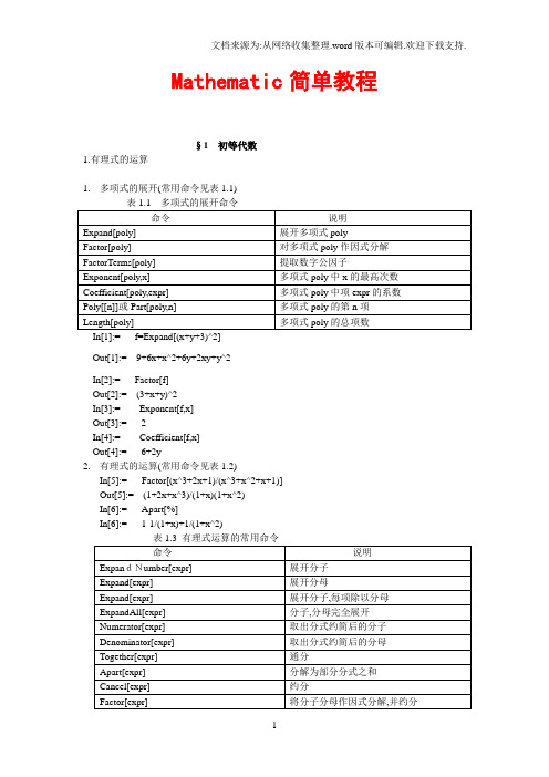
Mathematic简单教程§1 初等代数1.有理式的运算1.多项式的展开(常用命令见表1.1)In[1]:= f=Expand[(x+y+3)^2]Out[1]:= 9+6x+x^2+6y+2xy+y^2In[2]:= Factor[f]Out[2]:= (3+x+y)^2In[3]:= Exponent[f,x]Out[3]:= 2In[4]:= Coefficient[f,x]Out[4]:= 6+2y2.有理式的运算(常用命令见表1.2)In[5]:= Factor[(x^3+2x+1)/(x^3+x^2+x+1)]Out[5]:= (1+2x+x^3)/(1+x)(1+x^2)In[6]:= Apart[%]In[6]:= 1-1/(1+x)+1/(1+x^2)3.多项式的代数运算(常用命令见表1.3)In[7]:=PolynomialQuotient[1+x^2,x+1,x]Out[7]:=-1+xIn[8]: =PolynomialGCD[x^2+2X+1,x^3+1,x^5+1]Out[8]:=1+x1.2 方程求解In[1]:=Solve[a*x+b==0,x]Out[1]={{x->-b/a}}In[2]:=Reduce[a*x+b==0,x]Out[2]= b==0&&a==0\\a≠0&&x==-b/aIn[3]: = FindRoot[Sin[x]==0,{x,3}]Out[3]= {x->3.14159}In[4]:= FindRoot[Sin[x]==0,{x,{6,6.5}}]Out[4]= {x->6.28319}In[5]:= FindRoot[{2^x+y^2==4,x^2+Sin[y]==1},{x,0},{y,0}]2微积分In[1]: = Limit[Sin[x]/x,x->0]Out[1]=1In[2]:=DI[Sin[n*x],x]Out[2]=nCos[nx]微积分的常用命令如表1.5所示,下面是一些例子。
mathematica简明使用教程

mathematica简明使用教程Mathematica是一种强大的数学软件,广泛应用于科学研究、工程计算和数据分析等领域。
本文将简要介绍Mathematica的使用方法,帮助读者快速上手。
一、安装和启动Mathematica我们需要下载并安装Mathematica软件。
在安装完成后,可以通过桌面图标或开始菜单中的快捷方式来启动Mathematica。
二、界面介绍Mathematica的界面分为菜单栏、工具栏、输入区域和输出区域四部分。
菜单栏提供了各种功能选项,工具栏包含了常用的工具按钮,输入区域用于输入代码或表达式,而输出区域则显示执行结果。
三、基本操作1. 输入和输出在输入区域输入代码或表达式后,按下Shift+Enter键即可执行,并在输出区域显示结果。
Mathematica会自动对输入进行求解或计算,并返回相应的输出结果。
2. 变量定义可以使用等号“=”来定义变量。
例如,输入“a = 3”,然后执行,就会将3赋值给变量a。
定义的变量可以在后续的计算中使用。
3. 函数调用Mathematica内置了许多常用的数学函数,可以直接调用使用。
例如,输入“Sin[π/2]”,然后执行,就会返回正弦函数在π/2处的值。
4. 注释和注解在代码中添加注释可以提高代码的可读性。
在Mathematica中,可以使用“(*注释内容*)”的格式来添加注释。
四、数学运算Mathematica支持各种数学运算,包括基本的加减乘除,以及更复杂的求导、积分、矩阵运算等。
下面简要介绍几个常用的数学运算:1. 求导可以使用D函数来求导。
例如,输入“D[Sin[x], x]”,然后执行,就会返回正弦函数的导数。
2. 积分可以使用Integrate函数来进行积分运算。
例如,输入“Integrate[x^2, x]”,然后执行,就会返回x的平方的不定积分。
3. 矩阵运算Mathematica提供了丰富的矩阵运算函数,可以进行矩阵的加减乘除、转置、求逆等操作。
mathematica简明教程

6、定义变量
Mathematica系统里定义的变量是以字 母开头的字母数字串表示,没有长度限 制 。变量名不能以数字开头。如x2可以 作为变量名。但是2x却是2*x的意思。 一般的格式为:
1) 2)
x=value :表示把值value赋给x x=y=value:表示把值value赋给x和y
7、清除变量
(1)常用函数的命令格式
三角函数 :Sin[x],Cos[x] ,Tan[x] ,Cot[x] 等 反三角函数 :ArcSin[x] ,ArcCos[x] , ArcTan[x]等 双曲函数与反双曲函数 :Sinh[x] ,Cosh[x] , Tanh[x],ArcSinh[x],ArcCosh[x],ArcTanh[x] 指数函数E^x(或Exp[x]),指数函数a^x 对数函数ln x用Log[x],以a为底的对数函数用 Log[a,x] 平方根函数 :Sqrt[x] ,绝对值函数 :Abs[x] 最大值函数:Max[a,b,c] 最小值函数:Min[a,b,c]
1197388020 5713814277 4740573255 4261354898 5943198204 0405273437 5 9251031023 1501362932 1
3、浮点数(实数)
浮点数的运算符与整数、有理数的运算符一样。两 个浮点数运算或一个浮点数与一个整数(有理数) 运算,得到的结果都是浮点数.Mathematica可以将 整数、有理数转换为浮点数,可以得到它们的任意 位有效数字的浮点表示,转换是用一个系统函数: 大写的N[x,n].如 N[237/4683, 50]:表示取 237/4683的50位近似值。方括号中的两项用逗号分 隔开,第一项是被取值的数或式子,第二项是要求 的近似值位数 。如果只想求近似值而不关心位数, 可以写 N[237/4683]或237/4683 //N
Mathematica使用教程
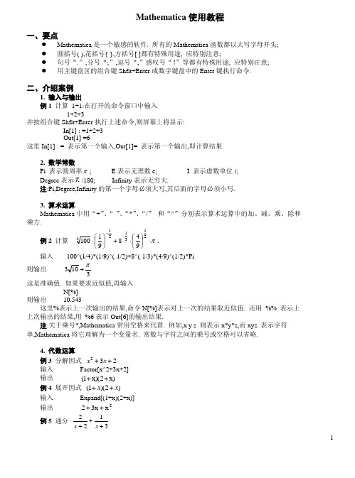
Mathematica 使用教程一、要点● Mathematica 是一个敏感的软件. 所有的Mathematica 函数都以大写字母开头;● 圆括号( ),花括号{ },方括号[ ]都有特殊用途, 应特别注意;● 句号“.”,分号“;”,逗号“,”感叹号“!”等都有特殊用途, 应特别注意;● 用主键盘区的组合键Shfit+Enter 或数字键盘中的Enter 键执行命令.二、介绍案例1. 输入与输出例1 计算 1+1:在打开的命令窗口中输入1+2+3并按组合键Shfit+Enter 执行上述命令,则屏幕上将显示:In[1] : =1+2+3Out[1] =6这里In[1] : = 表示第一个输入,Out[1]= 表示第一个输出,即计算结果.2. 数学常数Pi 表示圆周率π; E 表示无理数e; I 表示虚数单位i ;Degree 表示π/180; Infinity 表示无穷大.注:Pi,Degree,Infinity 的第一个字母必须大写,其后面的字母必须小写.3. 算术运算Mathematica 中用“+”、“-”、“*”、“/” 和“^”分别表示算术运算中的加、减、乘、除和乘方.例2 计算 π⋅⎪⎭⎫ ⎝⎛⋅+⎪⎭⎫ ⎝⎛⋅--213121494891100.输入 100^(1/4)*(1/9)^(-1/2)+8^(-1/3)*(4/9)^(1/2)*Pi则输出 3103π+这是准确值. 如果要求近似值,再输入N[%]则输出 10.543这里%表示上一次输出的结果,命令N[%]表示对上一次的结果取近似值. 还用 %% 表示上上次输出的结果,用 %6表示Out[6]的输出结果.注:关于乘号*,Mathematica 常用空格来代替. 例如,x y z 则表示x*y*z,而xyz 表示字符串,Mathematica 将它理解为一个变量名. 常数与字符之间的乘号或空格可以省略.4. 代数运算例3 分解因式 232++x x输入 Factor[x^2+3x+2]输出 )x 2)(x 1(++例4 展开因式 )2)(1(x x ++输入 Expand[(1+x)(2+x)]输出 2x x 32++例5 通分 3122+++x x输入 Together[1/(x+3)+2/(x+2)]输出 )x 3)(x 2(x 38+++ 例6 将表达式)3)(2(38x x x +++ 展开成部分分式 输入 Apart[(8+3x)/((2+x)(3+x))]输出 3x 12x 2+++ 例7 化简表达式 )3)(1()2)(1(x x x x +++++输入 Simplify[(1+x)(2+x)+(1+x)(3+x)] 输出 2x 2x 75++三、部分函数1. 内部函数Mathematica 系统内部定义了许多函数,并且常用英文全名作为函数名,所有函数名的第一个字母都必须大写,后面的字母必须小写. 当函数名是由两个单词组成时,每个单词的第一个字母都 必须大写,其余的字母必须小写. Mathematica 函数(命令)的基本格式为函数名[表达式,选项]下面列举了一些常用函数: 算术平方根x Sqrt[x]指数函数x eExp[x] 对数函数x a logLog[a,x] 对数函数x lnLog[x] 三角函数Sin[x], Cos[x], Tan[x], Cot[x], Sec[x], Csc[x] 反三角函数 ArcSin[x], ArcCos[x], ArcTan[x],ArcCot[x], AsrcSec[x], ArcCsc[x]双曲函数 Sinh[x], Cosh[x], Tanh[x],反双曲函数 ArcSinh[x], ArcCosh[x], ArcTanh[x]四舍五入函数 Round[x] (*取最接近x 的整数*)取整函数 Floor[x] (*取不超过x 的最大整数*)取模 Mod[m,n] (*求m/n 的模*)取绝对值函数 Abs[x]n 的阶乘 n!符号函数 Sign[x]取近似值 N[x,n] (*取x 的有n 位有效数字的近似值,当n 缺省时,n 的默认值为6*)例8 求π的有6位和20位有效数字的近似值.输入 N[Pi] 输出 3.14159输入 N[Pi, 20] 输出 3.1415926535897932285注:第一个输入语句也常用另一种形式:输入 Pi//N 输出 3.14159例9 计算函数值(1) 输入 Sin[Pi/3] 输出23(2) 输入 ArcSin[.45] 输出 0.466765(3) 输入 Round[-1.52] 输出 -2例10 计算表达式 )6.0arctan(226sin 2ln 1132+-+-e π 的值输入 1/(1+Log[2])*Sin[Pi/6]-Exp[-2]/(2+2^(2/3))*ArcTan[.6]输出 0.2749212. 自定义函数在Mathematica 系统内,由字母开头的字母数字串都可用作变量名,但要注意其中不能包含空格或标点符号.变量的赋值有两种方式. 立即赋值运算符是“=”,延迟赋值运算符是“: =”. 定义函数使用的符号是延迟赋值运算符“: =”.例11 定义函数 12)(23++=x x x f ,并计算)2(f ,)4(f ,)6(f .输入Clear[f,x]; (*清除对变量f 原先的赋值*)f[x_]:=x^3+2*x^2+1; (*定义函数的表达式*)f[2] (*求)2(f 的值*)f[x]/.{x->4} (*求)4(f 的值,另一种方法*)x=6; (*给变量x 立即赋值6*)f[x] (*求)6(f 的值,又一种方法*)输出1797289注:本例1、2、5行的结尾有“;”,它表示这些语句的输出结果不在屏幕上显示.四、解方程在Mathematica 系统内,方程中的等号用符号“==”表示. 最基本的求解方程的命令为Solve[eqns, vars]它表示对系数按常规约定求出方程(组)的全部解,其中eqns 表示方程(组),vars 表示所求未知变量.例12 解方程0232=++x x输入 Solve[x^2+3x+2==0, x]输出 }}1x {},2x {{-→-→例13 解方程组 ⎩⎨⎧=+=+10dy cx by ax 输入 Solve[{a x + b y == 0,c x + d y ==1}, {x,y}]输出 ⎭⎬⎫⎩⎨⎧⎭⎬⎫⎩⎨⎧+-→-→ad bc a y ,ad bc b x 例14 解无理方程a x x =++-11输入 Solve[Sqrt[x-1]+ Sqrt[x+1] == a, x]输出 ⎪⎭⎪⎬⎫⎪⎩⎪⎨⎧⎪⎭⎪⎬⎫⎪⎩⎪⎨⎧+→24a 4a 4x很多方程是根本不能求出准确解的,此时应转而求其近似解. 求方程的近似解的方法有两种,一种是在方程组的系数中使用小数,这样所求的解即为方程的近似解;另一种是利用下列专门用于求方程(组)数值解的命令:NSolve[eqns, vars] (*求代数方程(组)的全部数值解*)FindRoot[eqns, {x, x0}, {y, y0}Λ,]后一个命令表示从点),,(00Λy x 出发找方程(组)的一个近似解,这时常常需要利用图像法先大致确定所求根的范围,是大致在什么点的附近.例15 求方程013=-x 的近似解输入 NSolve[x^3-1== 0, x]输出 {{→x -0.5-0.866025ii},{→x -0.5+0.866025ii},{→x 1.}}输入 FindRoot[x^3-1==0,{x, .5}]输出 {→x 1.}下面再介绍一个很有用的命令:Eliminate[eqns, elims] (*从一组等式中消去变量(组)elims*)例16从方程组 ⎪⎩⎪⎨⎧=+=-+-+=++11)1()1(1222222y x z y x z y x 消去未知数y 、z .输入Eliminate[{x^2+y^2+z^2 ==1,x^2+(y-1)^2 + (z-1)^2 ==1, x + y== 1},{y, z}]输出 0x 3x 22==+-注:上面这个输入语句为多行语句,它可以像上面例子中那样在行尾处有逗号的地方将行与行隔开, 来迫使Mathematica 从前一行继续到下一行在执行该语句. 有时候多行语句的意义不太明 确,通常发生在其中有一行本身就是可执行的语句的情形,此时可在该行尾放一个继续的记号“\”, 来迫使Mathematica 继续到下一行再执行该语句.五、保存与退出Mathematica 很容易保存Notebook 中显示的内容,打开位于窗口第一行的File 菜单,点击Save后得到保存文件时的对话框,按要求操作后即可把所要的内容存为 *.nb 文件. 如果只想保存全部 输入的命令,而不想保存全部输出结果,则可以打开下拉式菜单Kernel,选中Delete All Output,然后 再执行保存命令. 而退出Mathematica 与退出Word 的操作是一样的.六、查询与帮助查询某个函数(命令)的基本功能,键入“?函数名”,想要了解更多一些,键入“??函数名”,例如,输入?Plot则输出Plot[f,{x,xmin,xmax}] generates a plot of f as a functionof x from xmin to xmax. Plot[{f1,f2,…},{x,xmin,xmax}] plots several functions fi它告诉了我们关于绘图命令“Plot ”的基本使用方法.例17 在区间]1,1[-上作出抛物线2x y =的图形.输入 Plot[x^2,{x,-1,1}]则输出-1-0.50.510.20.40.60.81例18 π.输入 Plot[{Sin[x],Cos[x]},{x,0,2Pi}]则输出123456-1-0.50.51??Plot则Mathematica 会输出关于这个命令的选项的详细说明,请读者试之.此外,Mathematica 的Help 菜单中提供了大量的帮助信息,其中Help 菜单中的第一项HelpBrowser(帮助游览器)是常用的查询工具,读者若想了解更多的使用信息,则应自己通过Help 菜单去学习.编辑本段Mathematica 基本运算a+mathematica 数学实验(第2版)b+c 加a-b 减a b c 或a*b*c 乘a/b 除-a 负号a^b 次方Mathematica 数字的形式256 整数2.56 实数11/35 分数2+6I 复数常用的数学常数Pi 圆周率,π=3.141592654…E 尤拉常数,e=2.71828182…Degree 角度转换弧度的常数,Pi/180I 虚数,其值为√-1Infinity 无限大指定之前计算结果的方法% 前一个运算结果%% 前二个运算结果%%…%(n个%) 前n个运算结果%n 或Out[n] 前n个运算结果复数的运算指令a+bI 复数Conjugate[a+bI] 共轭复数Re[z], Im[z] 复数z的实数/虚数部分Abs[z] 复数z的大小或模数(Modulus)Arg[z] 复数z的幅角(Argument)Mathematica 输出的控制指令expr1; expr2; expr3 做数个运算,但只印出最後一个运算的结果expr1; expr2; expr3; 做数个运算,但都不印出结果expr; 做运算,但不印出结果编辑本段常用数学函数Sin[x],Cos[x],Tan[x],Cot[x],Sec[x],Csc[x] 三角函数,其引数的单位为弪度Sinh[x],Cosh[x],Tanh[x],… 双曲函数ArcSin[x],ArcCos[x],ArcTan[x] 反三角函数ArcCot[x],ArcSec[x],ArcCsc[x]Arc Sinh[x],ArcCosh[x],ArcTanh[x],… 反双曲函数Sqrt[x] 根号Exp[x] 指数Log[x] 自然对数Log[a,x] 以a为底的对数Abs[x] 绝对值Round[x] 最接近x的整数Floor[x] 小於或等於x的最大整数Ceiling[x] 大於或等於x的最小整数Mod[a,b] a/b所得的馀数n! 阶乘Random[] 0至1之间的随机数(最新版本已经不用这个函数,改为使用RandomReal[])Max[a,b,c,...],Min[a,b,c,…] a,b,c,…的极大/极小值编辑本段数之设定x=a 将变数x的值设为ax=y=b 将变数x和y的值均设为bx=. 或Clear[x] 除去变数x所存的值变数使用的一些法则xy 中间没有空格,视为变数xyx y x乘上y3x 3乘上xx3 变数x3x^2y 为x^2 y次方运算子比乘法的运算子有较高的处理顺序编辑本段四个常用处理代数的指令Expand[expr] 将expr展开Factor[expr] 将expr因式分解Simplify[expr] 将expr化简成精简的式子FullSimplify[expr] Mathematica 会尝试更多的化简公式,将expr化成更精简的式子编辑本段多项式/分式转换的函数ExpandAll[expr] 把算是全部展开Together[expr] 将expr各项通分在并成一项Apart[expr] 把分式拆开成数项分式的和Apart[expr,var] 视var以外的变数为常数,将expr拆成数项的和Cancel[expr] 把分子和分母共同的因子消去编辑本段分母/分子的运算Denominator[expr] 取出expr的分母Numerator[expr] 取出expr的分子ExpandDenominator[expr] 展开expr的分母ExpandNumerator[expr] 展开expr的分子编辑本段多项式的另二种转换函数Collect[expr,x] 将expr表示成x的多项式,如Collect[expr,{x,y,…}] 将expr分别表示成x,y,…的多项式FactorTerms[expr] 将expr的数值因子提出,如4x+2=2(2x+1)FactorTerms[expr,x] 将expr中把所有不包含x项的因子提出FactorTerms[expr,{x,y,…}] 将expr中把所有不包含{x,y,...}项的因子提出编辑本段三角函数、双曲函数和指数的运算TrigExpand[expr] 将三角函数展开TrigFactor[expr] 将三角函数所组成的数学式因式分解TrigReduce[expr] 将相乘或次方的三角函数化成一次方的基本三角函数之组合ExpToTrig[expr] 将指数函数化成三角函数或双曲函数TrigToExp[expr] 将三角函数或双曲函数化成指数函数复数、次方乘积之展开ComplexExpand[expr] 假设所有的变数都是实数来对expr展开ComplexExpand[expr,{x,y,…}] 假设x,y,..等变数均为复数来对expr展开PowerExpand[expr] 将多项式项次、系数与最高次方之取得Coefficient[expr,form] 於expr中form的系数Exponent[expr,form] 於expr中form的最高次方Part[expr,n] 或expr[[n]] 在expr项中第n个项代换运算子expr/.x->value 将expr里所有的x均代换成valueexpr/.{x->value1,y->value2,…} 执行数个不同变数的代换expr/.{{x->value1},{x->value2},…} 将expr代入不同的x值expr//.{x->value1,y->value2,…} 重复代换到expr不再改变为止求解方程式的根Solve[lhs==rhs,x] 解方程式lhs==rhs,求xNsolve[lhs==rhs,x] 解方程式lhs==rhs的数值解Solve[{lhs1==rhs1,lhs2==rhs2,…},{x,y,…}] 解联立方程式,求x,y,…NSolve[{lhs1==rhs1,lhs2==rhs2,…},{x,y,…}] 解联立方程式的数值解FindRoot[lhs==rhs,{x,x0}] 由初始点x0求lhs==rhs的根Mathematica 的四种括号(term) 圆括号,括号内的term先计算f[x] 方括号,内放函数的引数{x,y,z} 大括号或串列括号,内放串列的元素p[[i ]] 或Part[p,i] 双方括号,p的第i项元素p[[i,j]] 或Part[p,i,j] p的第i项第j个元素缩短Mathematica输出的指令expr//Short 显示一行的计算结果Short[expr,n] 显示n行的计算结果Command; 执行command,但不列出结果查询Mathematica的物件?Command 查询Command的语法及说明??Command 查询Command的语法和属性及选择项?Aaaa* 查询所有开头为Aaaa的物件函数的定义、查询与清除f[x_]= expr 立即定义函数f[x]f[x_]:= expr 延迟定义函数f[x]f[x_,y_,…] 函数f有两个以上的引数?f 查询函数f的定义Clear[f] 或f=. 清除f的定义Remove[f] 将f自系统中清除掉含有预设值的Patterna_+b_. b的预设值为0,即若b从缺,则b以0代替x_ y_ y的预设值为1x_^y_ y的预设值为1条件式的自订函数lhs:=rhs/;condition 当condition成立时,lhs才会定义成rhsIf指令If[test,then,else] 若test为真,则回应then,否则回应elseIf[test,then,else,unknow] 同上,若test无法判定真或假时,则回应unknow 极限Limit[expr,x->c] 当x趋近c时,求expr的极限Limit[expr,x->c,Direction->1]Limit[expr,x->c,Direction->-1]微分D[f,x] 函数f对x作微分D[f,x1,x2,…] 函数f对x1,x2,…作微分D[f,{x,n}] 函数f对x微分n次D[f,x,NonConstants->{y,z,…}] 函数f对x作微分,将y,z,…视为x的函数全微分Dt[f] 全微分dfDt[f,x] 全微分Dt[f,x1,x2,…] 全微分Dt[f,x,Constants->{c1,c2,…}] 全微分,视c1,c2,…为常数不定积分Integrate[f,x] 不定积分∫f dx定积分Integrate[f,{x,xmin,xmax}] 定积分Integrate[f,{x,xmin,xmax},{y,ymin,ymax}] 定积分数列之和与积Sum[f,{i,imin,imax}] 求和Sum[f,{i,imin,imax,di}] 求数列和,引数i以di递增Sum[f,{i,imin,imax},{j,jmin,jmax}]Product[f,{i,imin,imax}] 求积Product[f,{i,imin,imax,di}] 求数列之积,引数i以di递增Product[f,{i,imin,imax},{j,jmin,jmax}]函数之泰勒展开式Series[expr,{x,x0,n}] 对expr於x0点作泰勒级数展开至(x-x0)n项Series[expr,{x,x0,m},{y,y0,n}] 对x0和y0展开关系运算子a==b 等於a>b 大於a>=b 大於等於a<b 小於a<=b 小於等於a!=b 不等於逻辑运算子!p notp||q||… orp&&q&&… andXor[p,q,…] exclusive orLogicalExpand[expr] 将逻辑表示式展开基本二维绘图指令Plot[f,{x,xmin,xmax}]画出f在xmin到xmax之间的图形Plot[{f1,f2,…},{x,xmin,xmax}]同时画出数个函数图形Plot[f,{x,xmin,xmax},option->value]指定特殊的绘图选项,画出函数f的图形Plot[]几种常用选项的指令选项预设值说明AspectRatio 1/GoldenRatio 图形高和宽之比例,高/宽Axes True 是否把坐标轴画出AxesLabel Automatic 为坐标轴贴上标记,若设定为AxesLabel->{?ylabel?},则为y轴之标记。
数学软件Mathematica详解教程

生成 n 元列表 {expr,expr,...,expr}
{expr|i 在列表 list 中变化}
Table[expr,{i,a,b,h}] {expr|i 在 Range[a,b,h]中变化}
Table 中的 expr 一般给的是通项公式
RandomInteger[range,n] 生成 n 个伪随机整数,range 表示取值范围
ToExpression[str]
ToString[expr]
转化为表达式
将表达式转化为字符串
更多字符串相关函数参见 “参考资料中心”
26
列表
列表
是 Mathematica 的基本对象,可用来表示集合,数组等 分为标准列表和稀疏列表
标准列表: 用大括号括起来的有限个元素,元素之间用逗号分隔
求最大值
求最小值
19
常用初等函数
Re[x], Im[x]
Conjugate[x] Arg[x]
提取实部和虚部
取共轭 辐角
Mod[m,n]
Quotient[m,n] Sin[x], Cos[x], ... ArcSin[x], ArcCos[x], ... Sinh, Cosh, ...,
m 除以 n 的余数
In[1]:= Clear[x,y]; In[2]:= f=2*x+y; In[3]:= f./{x->2,y->3} (* f(2,3) 的值 *)
In[3]:= f./{2->5}
(*把 2 替换成 5*)
15
数的基本运算
Mathematica 中的实数分精确数和双精度数
N[x,n] N[x] IntegerPart[x] FractionalPart[x] Floor[x] Round[x] Ceil[x] Precision[expr] x 的带 n 位有效数字的近似值 x 的双精度近似值 整数部分 小数部分 取整:不大于 x 的最大整数 取整:四舍五入 取整:不小于 x 的最小整数 显示计算精度
Mathematica 简明教程
A Tutorial Introduction to MathematicaAims and Objectives•To provide a tutorial guide to Mathematica.•To give practical experience in using the package.•To promote self-help using the online help facilities.•To provide a concise reference source for experienced users.On completion of this chapter the reader should be able to•use Mathematica as a tool;•produce simple Mathematica notebooks;•access some Mathematica commands and notebooks over the World Wide Web.It is assumed that the reader is familiar with either the Windows or UNIX platform.This book was prepared using Mathematica(Version6.0)but most pro-grams should work under earlier and later versions of the package.Note that the online version of the Mathematica commands for this book will be written using the most up-to-date version of the package.The command lines and programs listed in this chapter have been chosen to allow the reader to become familiar with Mathematica within a few hours.They20.A Tutorial Introduction to Mathematicaprovide a concise summary of the type of commands that will be used throughout the text.New users should be able to start on their own problems after completing the chapter,and experienced users shouldfind this chapter an excellent source of reference.Of course,there are many Mathematica textbooks on the market for those who require further applications or more detail.If you experience any problems there are several options for you to take. There is an excellent index within Mathematica,and Mathematica commands, notebooks,programs,and output can also be viewed in color over the Web at Mathematica’s Information Center:/infocenter/Books/AppliedMathematics/The notebookfiles can be found at the links Calculus Analysis and Dynamical Systems.Download the zipped notebookfiles and Extract the relevantfiles from the archive onto your computer.0.1A Quick Tour of MathematicaTo start Mathematica,simply double-click on the Mathematica icon.In the UNIX environment,one types mathematica as a shell command.The author has used the Windows platform in the preparation of this material.When Mathematica starts up,a blank notebook appears on the computer screen entitled Untitled-1and some palettes with buttons may appear alongside.Some examples of palettes are given in Figure0.1.The buttons on the palettes serve essentially as additional keys on the user keyboard.Input to the Mathematica notebook can either be performed by typing in text commands or pointing and clicking on the symbols provided by various palettes and subpalettes.As many of the Mathematica programs in subsequent chapters of this book are necessarily text based,the author has decided to present the material using commands in their text format.However,the use of palettes can save some time in typing,and the reader may wish to experiment with the“clicking on palettes’’approach.Mathematica even allows users to create their own palettes;again readers mightfind this useful.Mathematica notebooks can be used to generate full publication-quality doc-uments.In fact,all of the Mathematica help pages have been created with interac-tive notebooks.The Help menu also includes an online version of the Mathematica book[1].The author recommends a brief tour of some of the help pages to give the reader an idea of how the notebooks can be used.For example,click on the Help toolbar at the top of the Mathematica graphical user interface and scroll down to Help browser....Simply type in Solve and ENTER.An interactive Mathemat-ica notebook will be opened showing the syntax,some related commands,and examples of the Solve command.The interactive notebooks from each chapter of this book can be downloaded from Mathematica’s Information Center:/infocenter/Books/AppliedMathematics/0.1.A Quick Tour of Mathematica3(a)(b)(c)(d)Figure0.1:Some Mathematica palettes:(a)Basic input palette.(b)Technical symbols,shapes,and icons.(c)Relational operators.(d)Relational arrows.The author has provided the reader with a tutorial introduction to Mathematica in Sections0.2,0.3,and0.4.Each tutorial should take no more than one hour to complete.The author highly recommends that new users go through these tutorials line by line;however,readers already familiar with the package will probably use Chapter0as reference material only.Tutorial One provides a basic introduction to the Mathematica package. Thefirst command line shows the reader how to input comments,which are extremely useful when writing long or complicated programs.The reader will type in(*This is a comment*)and then type SHIFT-ENTER or SHIFT-RETURN (hold down the SHIFT key and press ENTER).Mathematica will label thefirst input with In[1]:=(*This is a comment*).Note that no output is given for a comment.The second input line is simple arithmetic.The reader types 2+3-36/2+2ˆ3,and types SHIFT-ENTER to compute the result.Mathematica labels the second input with In[2]:=2+3-36/2+2ˆ3,and labels the corre-sponding output Out[2]=-5.As the reader continues to input new command40.A Tutorial Introduction to Mathematicalines,the input and output numbers change accordingly.This allows users to easily label input and output that may be useful later in the notebook.Note that all of the built-in Mathematica functions begin with capital letters and that the arguments are always enclosed in square brackets.Tutorial Two contains graphic commands and commands used to solve simple differential equations.Tutorial Three pro-vides a simple introduction to the Manipulate command and programming with Mathematica.The tutorials are intended to give the reader a concise and efficient intro-duction to the Mathematica package.Many more commands are listed in other chapters of the book,where the output has been included.Of course,there are many Mathematica textbooks on the market for those who require further appli-cations or more detail.A list of textbooks is given in the reference section of this chapter.0.2Tutorial One:The Basics(One Hour)There is no need to copy the comments,they are there to help you.Click on the Mathematica icon and copy the commands.Hold down the SHIFT key and press ENTER at the end of a line to see the answer or use a semicolon to suppress the output.You can interrupt a calculation at any time by typing ALT-COMMA or COMMAND-COMMA.A working Mathematica notebook of Tutorial One can be downloaded from the Mathematica Information Center,as indicated at the start of the chapter.Mathematica Command Lines CommentsIn[1]:=(*This is a comment*)(*Helps when writingprograms.*)In[2]:=2+3-36/2+2ˆ3(*Simple arithmetic.*)In[3]:=23*7(*Use space or*tomultiply.*)In[4]:=2/3+4/5(*Fraction arithmetic.*)In[5]:=2/3+4/5//N(*Approximate decimal.*)In[6]:=Sqrt[16](*Square root.*)In[7]:=Sin[Pi](*Trigonometric function.*) In[8]:=z1=1+2I;z2=3-4*I;z3=z1-z2/z1(*Complex arithmetic.*)In[9]:=ComplexExpand[Exp[z1]](*Express in form x+iy.*)In[10]:=Factor[xˆ3-yˆ3](*Factorize.*)In[11]:=Expand[%](*Expand the last resultgenerated.*)In[12]:=f=mu x(1-x)/.{mu->4,x->0.2}(*Evaluate f when mu=4andx=0.2.*)In[13]:=Clear[mu,x](*Clear values.*)0.2.Tutorial One:The Basics(One Hour)5In[14]:=Simplify[(xˆ3-yˆ3)/(x-y)](*Simplify an expression.*) In[15]:=Dt[xˆ2-3x+6,x](*Total differentiation.*)In[16]:=D[xˆ3yˆ5,{x,2},{y,3}](*Partial differentiation.*) In[17]:=Integrate[Sin[x]Cos[x],x](*Indefinite integration.*) In[18]:=Integrate[Exp[-xˆ2],{x,0,Infinity}](*Definite integration.*)In[19]:=Sum[1/nˆ2,{n,1,Infinity}](*An infinite sum.*)In[20]:=Solve[xˆ2-5x+6==0,x](*Solving equations.Rootsare in a list.*)In[21]:=Solve[xˆ2-5x+8==0,x](*A quadratic with complexroots.*)In[22]:=Abs[x]/.Out[21](*Find the modulus of theroots(see Out[21]).*)In[23]:=Solve[{xˆ2+yˆ2==1,x+3y==0}](*Solving simultaneousequations.*)In[24]:=Series[Exp[x],{x,0,5}](*Taylor series expansion.*) In[25]:=Limit[x/Sin[x],x->0](*Limits.*)In[26]:=f=Function[x,4x(1-x)](*Define a function.*)In[27]:=f[0.2](*Evaluate f(0.2).*)In[28]:=fofof=Nest[f,x,3](*Calculates f(f(f(x))).*)In[29]:=fnest=NestList[f,x,4](*Generates a list ofcomposite functions.*)In[30]:=fofofof=fnest[[4]](*Extract the4th elementof the list.*)In[31]:=u=Table[2i-1,{i,5}](*List the first5oddnatural numbers.*)In[32]:=%ˆ2(*Square the elements ofthe last result generated.*) In[33]:=a={2,3,4};b={5,6,7};(*Two vectors.*)In[34]:=3a(*Scalar multiplication.*)In[35]:=a.b(*Dot product.*)In[36]:=Cross[a,b](*Cross product.*)In[37]:=Norm[a](*Norm of a vector.*)In[38]:=A={{1,2},{3,4}};B={{5,6},{7,8}};(*Two matrices.*)In[39]:=A.B-B.A(*Matrix arithmetic.*)In[40]:=MatrixPower[A,3](*Powers of a matrix.*)In[41]:=Inverse[A](*The inverse of a matrix.*) In[42]:=Det[B](*The determinant of amatrix.*)60.A Tutorial Introduction to MathematicaIn[43]:=Tr[B](*The trace of a matrix.*) In[44]:=M={{1,2,3},{4,5,6},{7,8,9}}(*A matrix.*)In[45]:=Eigenvalues[M](*The eigenvalues of amatrix.*)In[46]:=Eigenvectors[M](*The eigenvectors of amatrix.*)In[47]:=LaplaceTransform[tˆ3,t,s](*Laplace transform.*)In[48]:=InverseLaplaceTransform[6/sˆ4,s,t](*Inverse Laplacetransform.*)In[49]:=FourierTransform[tˆ4Exp[-tˆ2],t,w](*Fourier transform.*)In[50]:=InverseFourierTransform[%,w,t](*Inverse Fouriertransform.*)In[51]:=Quit[](*Terminates Mathematicakernel session.*)0.3Tutorial Two:Plots and Differential Equations(One Hour)Mathematica has excellent graphical capabilities and many solutions of nonlinear systems are best portrayed graphically.The graphs produced from the input text commands listed below may be found in the Tutorial Two Notebook which can be downloaded from the Mathematica Information Center.Plots in other chapters of the book are referred to in many of the Mathematica programs at the end of each chapter.(*Plotting graphs.*)(*Set up the domain and plot a simple function.*)In[1]:=Plot[Sin[x],{x,-Pi,Pi}](*Plot two curves on one graph.*)In[2]:=Plot[{Cos[x],Exp[-.1x]Cos[x]},{x,0,60}](*Plotting with labels.*)In[3]:=Plot[Exp[-.1t]Sin[t],{t,0,60},AxesLabel->{"t","Current"},PlotRange->{-1,1}](*Contour plot with shading.*)In[4]:=ContourPlot[yˆ2/2-xˆ2/2+xˆ4/4,{x,-2,2},{y,-2,2}](*Contour plot with no shading.*)In[5]:=ContourPlot[yˆ2/2-xˆ2/2+xˆ4/4,{x,-2,2},{y,-2,2},0.3.Tutorial Two:Plots and Differential Equations(One Hour)7ContourShading->False](*Contour plot with20contours.*)In[6]:=ContourPlot[yˆ2/2-xˆ2/2+xˆ4/4,{x,-2,2},{y,-2,2}, Contours->20](*Surface plot.*)In[7]:=Plot3D[yˆ2/2-xˆ2/2+xˆ4/4,{x,-2,2},{y,-2,2}](*A parametric plot.*)In[8]:=ParametricPlot[{tˆ3-4t,tˆ2},{t,-3,3}](*3-D parametric curve.*)In[9]:=ParametricPlot3D[{Sin[t],Cos[t],t/3},{t,-10,10}](*Load the package and plot an implicit curve.*)In[10]:=<<Graphics‘ImplicitPlot‘In[11]:=ImplicitPlot[2xˆ2+3yˆ2==12,{x,-3,3},{y,-3,3}](*Solve a simple separable differential equation.*)In[12]:=DSolve[x’(t)==-x[t]/t,x[t],t](*Solve an initial value problem(IVP).*)In[13]:=DSolve[{x’(t)==-t/x[t],x[0]==1},x[t],t](*Solve a second-order ordinary differential equation (ODE).*)In[14]:=DSolve[{x’’[t]+5x’[t]+6x[t]==10Sin[t],x[0]==0, x’[0]==0},x[t],t](*Solve a system of two ODEs.*)In[15]:=DSolve[{x’[t]==3x[t]+4y[t],y’[t]==-4x[t]+3y[t]}, {x[t],y[t]},t](*Solve a system of three ODEs.*)In[16]:=DSolve[{x’[t]==x[t],y’[t]==y[t],z’[t]==-z[t]}, {x[t],y[t],z[t]},t](*Solve an IVP using numerical methods and plot a solution curve.*)In[17]:=u=NDSolve[{x’[t]==x[t](.1-.01x[t]),x[0]==50}, x,{t,0,100}]In[18]:=Plot[Evaluate[x[t]/.u],{t,0,100},PlotRange->All](*Plot a phase plane portrait.*)In[19]:=v=NDSolve[{x’[t]==.1x[t]+y[t],y’[t]==-x[t]+.1y[t], x[0]==.01,y[0]==0},{x[t],y[t]},{t,0,50}]80.A Tutorial Introduction to MathematicaIn[20]:=ParamericPlot[{x[t],y[t]}/.v,{t,0,50},PlotRange->All,PlotPoints->1000](*Plot a three-dimensional phase portrait.*)In[21]:=w=NDSolve[{x’[t]==z[t]-x[t],y’[t]==-y[t],z’[t] ==z[t]-17x[t]+16,x[0]==.8,y[0]==.8,z[0]==.8},{x[t],y[t],z[t]},{t,0,20}]In[22]:=ParametricPlot3D[Evaluate[{x[t],y[t],z[t]}/.w], {t,0,20},PlotPoints->1000,PlotRange->All](*A stiff van der Pol system of ODEs.*)In[23]:=Needs["DifferentialEquations‘InterpolatingFunctionAnatomy‘"];In[24]:=vanderpol=NDSolve[{Derivative[1][x][t]==y[t],Derivative[1][y][t]==1000*(1-x[t]ˆ2)*y[t]-x[t],x[0]==2,y[0]==0},{x,y},{t,5000}];In[25]:=T=First[InterpolatingFunctionCoordinates[First[x/.vanderpol]]];In[26]:=ListPlot[Transpose[{x[T],y[T]}/.First[vanderpol]], PlotRange->All]0.4The Manipulate Command and SimpleMathematica ProgramsSections0.1,0.2,and0.3illustrate the interactive nature of Mathematica.More involved tasks will require more code.Note that Mathematica is very different from procedural languages such as C,Pascal,or Fortran.An afternoon spent browsing through the pages listed at the Mathematica Information Center will convince readers of this fact.The Manipulate command is new in Version6.0and is very useful in the field of dynamical systems.Manipulate[expr,{u,u min,u max}]generates a version of expr with controls added to allow interactive manipulation of the value of u.The Manipulate CommandOn execution of the Manipulate command a parameter slider appears in the note-book.Solutions change as the slider is moved left and right.(*Example1:Solving simultaneous equations as the parameter a varies.See Exercise6in Chapter 3.*)In[1]:=Manipulate[Solve[{x(1-y-a x)==0,y(-1+x-a y)==0}], {a,0,1}](*Showing the solution lying wholly in the first quadrant.*) In[2]:=Manipulate[Plot[{1-a x,(x-1)/a},{x,0,2}],{a,0.01,1}]0.4.The Manipulate Command and Simple Mathematica Programs 9(*Example 2:Evaluating functions of functions to the fifth iteration.*)In[3]:=f=Function[x,4x (1-x)];In[4]:=Manipulate[Expand[Nest[f,x,d]],{d,1,5,1}](*Stepsof 1.*)(*Example 3:Solving a differential equation as twoparameters vary.In this case,the damping and restoring terms when modeling a simple pendulum.*)In[5]:=Manipulate[DSolve[{x’’[t]+b x’[t]+c x[t]==0,x[0]==1,x’[0]==0},x[t],t],{b,0,2},{c,0,5}](*The solution curves.*)In[6]:=Manipulate[soln=NDSolve[{x’’[t]+b x’[t]+c x[t]==0,x[0]==1,x’[0]==0},x[t],{t,0,100}];Plot[Evaluate[x[t]/.soln],{t,0,100},PlotRange->All],{b,0,5},{c,0,5}]Many Manipulate demonstrations are available from the Wolfram Demon-strations Project:/Simple Mathematica ProgramsEach Mathematica program is displayed between horizontal lines and kept short to aid in understanding;the output is also included.Modules and local variables.Aglobal variable t is unaffected by the local variable t used in a module.In[1]:=Norm3d[a_,b_,c_]=Module[{t},t=Sqrt[aˆ2+bˆ2+cˆ2]]Out [1]= a 2+b 2+c 2In[2]:=Norm3d[3,4,5]Out [2]=5√2The Do command.The first ten terms of the Fibonacci sequence.In[3]:=F[1]=1;F[2]=1;Nmax=10;In[4]:=Do[F[i]=F[i-1]+F[i-2],{i,3,Nmax}]In[5]:=Table[F[i],{i,1,Nmax}]Out [5]={1,1,2,3,5,8,13,21,34,55}100.A Tutorial Introduction to MathematicaIf,then,else construct.In[6]:=Num=1000;If[Num>0,Print["Num is positive"],If[Num==0, Print["Num is zero"],Print["Num is negative"]]]Out[6]=Num is positiveConditional statements with more than two alternatives.In[7]:=r[x_]=Switch[Mod[x,3],0,a,1,b,2,c]Out[7]=Switch[Mod[x,3],0,a,1,b,2,c]In[8]:=r[7]Out[8]=bWhich.Defining the tent function.In[9]:=T[x_]=Which[0<=x<1/2,mu x,1/2<=x<=1,mu(1-x)]Out[9]=Which[0≤x<1/2,mu x,1/2≤x≤1,mu(1−x)]In[10]:=T[4/5]Out[10]=mu5For pute f(x),f(f(x)),and f(f(f(x))).In[11]:=For[i=1;t=x,i<4,i++,t=mu t(1-t);Print[Factor[t]]] Out[11]=−mu(−1+x)x−mu2(−1+x)x(1−mu x+mu x2)−mu3(−1+x)x(1−mu x+mu x2)(1−mu2x+mu2x2+mu3x2−2mu3x3+mu3x4)Plotting solution curves.Solutions to the pendulum problem.See Figure0.2. In[12]:=ode1[x0_,y0_]:=NDSolve[{x’[t]==y[t],y’[t]==-25x[t], x[0]==x0,y[0]==y0},{x[t],y[t]},{t,0,6}];In[13]:=sol1[1]=ode1[1,0];In[14]:=ode2[x0_,y0_]:=NDSolve[{x’[t]==y[t],y’[t]==-2y[t]-25x[t],x[0]==x0,y[0]==y0},{x[t],y[t]},{t,0,6}];In[15]:=sol2[1]=ode2[1,0];In[16]:=p1=Plot[Evaluate[Table[{x[t]}/.sol1[i],{i,1}]], {t,0,6},PlotRange->All,PlotPoints->100,PlotStyle->Dashing[{.02}]];0.5.Hints for Programming 11123456t10.50.51xFigure 0.2:Harmonic and damped motion of a pendulum.In[17]:=p2=Plot[Evaluate[Table[{x[t]}/.sol2[i],{i,1}]],{t,0,6},PlotRange->All,PlotPoints->100];In[18]:=Show[{p1,p2},PlotRange->All,AxesLabel->{"t","x"},Axes->True,TextStyle->{FontSize->15}]0.5Hints for ProgrammingThe Mathematica language contains very powerful commands,which means that some complex programs may contain only a few lines of code.Of course,the only way to learn programming is to sit down and try it yourself.This section has been included to point out common errors and give advice on how to troubleshoot.Remember to check the help and index pages in Mathematica and the Web if the following does not help you with your particular problem.Common typing errors.The author strongly advises new users to type Tutorials One,Two,and Three into their own notebooks.This should reduce typing errors.•Type SHIFT-ENTER at the end of every command line.•If a command line is ended with a semicolon,the output will not be displayed.•Make sure brackets,parentheses,etc.,match up in correct pairs.•Remember that all of the built-in Mathematica functions begin with capital letters and that the arguments are always enclosed in square brackets.•Remember Mathematica is case sensitive.•Check the syntax;type ?Solve to list syntax for the Solve command,for example.120.A Tutorial Introduction to MathematicaProgramming tips.The reader should use the Mathematica programs listed in Section 0.4to practice simple programming techniques.•It is best to clear values at the start of a large program.•Use comments throughout a program.You will find them extremely useful in the future.•Use Modules or Blocks to localize variables.This is especially useful for very large programs.•If a program involves a large number of iterations,for example,50,000,then run it for three iterations first and list all output.•If the computer is not responding hold ALT-COMMA or COMMAND-COMMA and try reducing the size of the problem.•Read the error message printed by Mathematica and click on More…if necessary.•Find a similar Mathematica program in a book or on the Web,and edit it to meet your needs.•Check which version of Mathematica you are using.The syntax of some commands may have altered.0.6Mathematica Exercises1.Evaluate the following:(a)4+5−6;(b)312;(c)sin (0.1π);(d)(2−(3−4(3+7(1−(2(3−5))))));(e)25−34×23.2.Given thatA =⎛⎝12−10103−12⎞⎠,B =⎛⎝123112012⎞⎠,C =⎛⎝21101−1422⎞⎠,determine the following:(a)A +4BC ;(b)the inverse of each matrix if it exists;0.6.Mathematica Exercises 13(c)A 3;(d)the determinant of C ;(e)the eigenvalues and eigenvectors of B .3.Given that z 1=1+i ,z 2=−2+i ,and z 3=−i ,evaluate the following:(a)z 1+z 2−z 3;(b)z 1z 2z 3;(c)e z 1;(d)ln (z 1);(e)sin (z 3).4.Evaluate the following limits if they exist:(a)lim x →0sin x x ;(b)lim x →∞x 3+3x 2−52x 3−7x;(c)lim x →πcos x +1x −π;(d)lim x →0+1x;(e)lim x →02sinh x −2sin xcosh x −1.5.Find the derivatives of the following functions:(a)y =3x 3+2x 2−5;(b)y =√1+x 4;(c)y =e x sin x cos x ;(d)y =tanh x ;(e)y =x ln x .6.Evaluate the following definite integrals:(a) 1x =03x 3+2x 2−5dx ;(b) ∞x =11x 2dx ;(c) ∞−∞e −x 2dx ;(d) 101√xdx ;(e)2πsin (1/t)t 2dt .7.Graph the following:140.A Tutorial Introduction to Mathematica(a)y=3x3+2x2−5;(b)y=e−x2,for−5≤x≤5;(c)x2−2xy−y2=1;(d)z=4x2e y−2x4−e4y for−3≤x≤3and−1≤y≤1;(e)x=t2−3t,y=t3−9t for−4≤t≤4.8.Solve the following differential equations:(a)dydx =x2y,given that y(1)=1;(b)dydx =−yx,given that y(2)=3;(c)dydx =x2y3,given that y(0)=1;(d)d2xdt2+5dxdt+6x=0,given that x(0)=1and˙x(0)=0;(e)d2xdt2+5dxdt+6x=sin(t),given that x(0)=1and˙x(0)=0.9.Carry out100iterations on the recurrence relationx n+1=4x n(1−x n),given that(a)x0=0.2and(b)x0=0.2001.List thefinal10iterates in each case.10.Type?While to read the help page on the While e a whileloop to program Euclid’s algorithm forfinding the greatest common divisor of two e your program tofind the greatest common divisor of 12,348and14,238.Recommended Textbooks[1]S.Wolfram,The Mathematica Book,6th ed.(electronic),Wolfram Media,Champaign,IL,2007;included with Mathematica®Version6.0.[2]D.McMahon and D.M.Topa,A Beginner’s Guide to Mathematica,Chapmanand Hall,London,CA,2006.[3]G.Baumann,Mathematica for Theoretical Physics:Classical Mechanicsand Nonlinear Dynamics,Springer-Verlag,New York,2005.[4]G.Baumann,Mathematica for Theoretical Physics:Electrodynamics,Quan-tum Mechanics,General Relativity,and Fractals,Springer-Verlag,New York,2005.[5]M.Trott,The Mathematica Guidebook for Numerics,Springer-Verlag,NewYork,2005.Recommended Textbooks15 [6]M.Trott,The Mathematica Guidebook for Symbolics,Springer-Verlag,NewYork,2005.[7]M.Trott,The Mathematica Guidebook:Graphics,Springer-Verlag,NewYork,2004.[8]M.Trott,The Mathematica Guidebook:Programming,Springer-Verlag,New York,2004.[9]E.Don,Schaum’s Outline of Mathematica,McGraw–Hill,New York,2000.。
- 1、下载文档前请自行甄别文档内容的完整性,平台不提供额外的编辑、内容补充、找答案等附加服务。
- 2、"仅部分预览"的文档,不可在线预览部分如存在完整性等问题,可反馈申请退款(可完整预览的文档不适用该条件!)。
- 3、如文档侵犯您的权益,请联系客服反馈,我们会尽快为您处理(人工客服工作时间:9:00-18:30)。
Out[2]= 2469 1111
实数是用浮点数表示的,Mathematica 实数的有效位可取任意位数,是一种具有任意精
确度的近似实数,当然在计算的时候也可以控制实数的精度。实数有两种表示方法:一种是
小数,另外一种是用指数方法表示的。如:
In[3]:=0.239998
Out[3]=0.23998
In[4]:=0.12*10^11 Out[4]=0.12*10^11
1.3 Mathematica 的联机帮助系统
用 Mathematica 的过程中,常常需要了解一个命令的详细用法,或者想知系统中是否有 完成某一计算的命令,联机帮助系统永远是最详细、最方便的资料库。
1.获取函数和命令的帮助
在 Notebook 界面下,用 ?或 ?? 可向系统查询运算符、函数和命令的定义和用法,获 取简单而直接的帮助信息。 例如,向系统查询作图函数 Plot 命令的用法 ?Plot 系统将给 出调用 Plot 的格式以及 Plot 命令的功能(如果用两个问号 “??”, 则信息会更详细一 些)。? Plot* 给出所有以 Plot 这四个字母开头的命令。
1.2 表达式的输入
Mathematica 提供了多种输入数学表达式的方法。除了用键盘输入外, 还可以使用工 具样或者快捷方式健入运算符、矩阵或数学表达式。
1. 数学表达式二维格式的输入
Mathematic 担提供了两种格式的数学表达式。形如 x/(2+3x)+y*(x-w)的称为一维格式,
形如 x y 的称为二维格式。 2 3x x w
实数也可以与整数,有理数进行混合运算,结果还是一个实数。
In[5]:=2+1/4+0.5
Out[5]=2.75
小数表示
复数是由实部和虚部组成,实部和虚部可以用整数、实数、有理数表示。在 Mathematica
你可以使用快捷方式输入二维格式,也可用基本输入工具栏输入二维格式。下面列出了
用快捷方式输入二维格式的方法:
数学运算
数学表达式
按键
分式
x
2
n 次方
xnBiblioteka x Ctrl+/ 2 x Ctrl+^ n
开 2 次方
x
Ctrl +2 x
下标
x2
x Ctrl+_ 2
(x 1)4
例如输入数学表达式
,可以按如下顺序输入按键:
如果知道具体的函数名,但不知其详细使用说明,可以在命令按钮 Goto 右边的文本框中键
入函数名,按回 车键后就 显示有关函 数的定义、 例题和相关 联的章节 。例如,要 查找函数
Plot 的用法,只要在文本框中键入 Plot,按回车键后显示 Plot 函数的详细用法和例题的窗 口,如图 7。
图7 如果已经确知 Mathematica 中有具有某个功能的函数,但不知具体函数名,可以点击 Built-in Functions 按钮,再按功能分类从粗到细一步一步找到具体的函数,例如,要找 画一元函数图形的函数,点击 Built-in Functions →Graphics and Sound→2D Plots→ Plot,找到 Plot 的帮助信息(如图 7)。
图3 一个表达式只有准确无误,方能得出正确结果。学会看系统出错信息能帮助我们较快找 出错误,提高工作效率。 完成各种计算后,点击“文件”“退出” 退出,如果文件未存盘, 系统提示用户存盘,文件名以“.nb”作为后缀,称为 Notebook 文件。以后想使用本次保存 的结果时可以通过“文件”“打开”菜单读入,也可以直接双击它,系统自动调用 Mathematica 将它打开。
取 到 事半 功 倍的 效果 。 这些 函数 分 为两 类, 一类 是 数学 意义 上 的函 数, 如 :绝 对值 函 数 Abs[x],正弦函数 Sin[x],余弦函数 Cos[x],以 e 为底的对数函数 Log[x],以 a 为底的对 数 函 数 Log[a,x] 等 ; 第 二 类 是 命 令 意 义 上 的 函 数 , 如 作 函 数 图 形 的 函 数 Plot[f[x],{x,xmin,xmax}],解方程函数 Solve[eqn,x],求导函数 D[f[x],x]等。
8.1 运算符和一些特殊符号:常用的和不常用一些运算符号 8.2 系统常数:系统定义的一些常量及其意义 8.3 代数运算:表达式相关的一些运算函数 8.4 解方程:和方程求解有关的一些操作 8.5 微积分相关函数:关于求导,积分,泰勒展开等相关的函数 8.6 多项式函数:多项式的相关函数 8.7 随机函数:能产生随机数的函数函数 8.8 数值函数:和数值处理相关的函数,包括一些常用的数值算法 8.9 表相关函数:创建表,表元素的操作,表的操作函数 8.10 绘图函数:二维绘图,三维绘图,绘图设置,密度图,图元,着色,图
Getting Started/Demos 初学者入门指南/多种演示
Tour
漫游 Mathematic
Front End
菜单命令的快捷键,二维输入格式等
Master Index
按字母命令给出命令、函数和选项的索引表
如果要查找 Mathematica 中具有某个功能的函数,可以通过帮助菜单中的 Mahematica
第 2 章 Mathematica 的基本量
2.1 数据类型和常数
1.数值类型
在 Mathematic 中,基本的数值类型有四种:整数、有理数、实数和复数。
如果你的计算机的内存足够大,Mathemateic 可以表示任意长度的精确实数,而不受所
用的计算机字长的影响。整数与整数的计算结果仍是精确的整数或是有理数。例如 2 的 100
必 须 注 意的是: Mathematica 严格区分大小写,一般地,内建函数的首写字母必须大写,有时一个函数 名是由 几个 单词构 成, 则每 个单词 的首 写字 母也必 须大 写, 如:求 局部 极小 值函数 FindMinimum[f[x],{x,x0}等。第二点要注意的是,在 Mathematica 中,函数名和自变量之 间的分隔符是用方括号“[ ]”,而不是一般数学书上用的圆括号“( )”,初学者很容易犯这 类错误。 如果输入了不合语法规则的表达式,系统会显示出错信息,并且不给出计算结果,例如: 要画正弦函数在区间[-10,10]上的图形,输入 plot[Sin[x],{x,-10,10}],则系统提示“可 能有拼写错误, 新符号‘plot’ 很像已经存在的符号‘Plot’”, 实际上,系统作图命令 “Plot” 第一 个字 母必 须大 写, 一般 地,系 统内 建函 数首 写字 母都 要大 写。 再输入 Plot[Sin[x],{x,-10,10} ,系统又提示缺少右方括号,并且将不配对的括号用紫色显示, 如图 3。
次方是一个 31 位的整数:
ln[1]:=2^100 Out[1]=1267650600228228229401496703205376
在 Mathematica 中允许使用分数,也就是用有理数表示化简过的分数。当两个整数相除
而又不能整除时,系统就用有理数来表示,即有理数是由两个整数的比来组成如:
In[2]:=12345/5555
2x y
(,x,+,1,),Ctrl+ ^,+,4,→,Ctrl+/,Ctrl+2,2,x,+,y 另外也可从“文件”菜单中激活“控制面板”“Basic Input”工具栏,也可输入,并且
使用工具栏可输入更复杂的数学表达式,如下图 4。
图4
图5
2.特殊字符的输入
MathemMatica 还提供了用以输入各种特殊符号的工具栏。基本输入工具栏包含了常用 的特殊字符(上图),只要单击这些字符按钮即可输入。若要输入其它的特殊字符或运算符号, 必须使用从“文件”菜单中激活“控制面板”“Complete Characters”工具栏,如上图 5, 单击符号后即可输入。
3.1 多项式运算:多项的四则运算,多项式的化简等 3.2 方程求解:求解一般方程,条件方程,方程数值解以及方程组的求解 3.3 求积求和:求积与求和
第 4 章 函数作图
4.1 二维函数作图:一般函数的作图,参数方程的绘图 4.2 二维图形元素:点,线等图形元素的使用 4.3 图形样式:图形的样式,对图形进行设置 4.4 图形的重绘和组合:重新显示所绘图形,将多个图形组合在一起 4.5 三维图形的绘制:三维图形的绘制,三维参数方程的图形,三维图形的
图2 在 Mathematica 的 Notebook 界面下,可以用这种交互方式完成各种运算,如函数作图, 求极限、解方程等,也可以用它编写像 C 那样的结构化程序。在 Mathematica 系统中定义了 许多功能强大的函数,我们称之为内建函数(built-in function), 直接调用这些函数可以
形显示等函数 8.11 流程控制函数
第 1 章 Mathematica 概述
1.1 Mathematica 的启动和运行
Mathematica 是美国 Wolfram 研究公司生产的一种数学分析型的软件,以符号计算见长, 也具有高精度的数值计算功能和强大的图形功能。
假设在 Windows 环境下已安装好 Mathematica5.0,启动 Windows 后,在“开始”菜单
2.1 数据类型和常量:mathematica 中的数据类型和基本常量 2.2 变量:变量的定义,变量的替换,变量的清除等 2.3 函数:函数的概念,系统函数,自定义函数的方法 2.4 表:表的创建,表元素的操作,表的应用 2.5 表达式:表达式的操作 2.6 常用符号:经常使用的一些符号的意义
第 3 章 Mathematica 的基本运算
设置
第 5 章 微积分的基本操作
5.1 函数的极限:如何求函数的极限 5.2 导数与微分:如何求函数的导数,微分 5.3 定积分与不定积分:如何求函数的不定积分和定积分,以及数值积分 5.4 多变量函数的微分:如何求多元函数的偏导数,微分 5.5 多变量函数的积分:如何计算重积分 5.6 无穷级数:无穷级数的计算,敛散性的判断