0909121405-雷亦恺-模式识别与机器学习实验报告(ex01&ex02)
模式识别 实验报告一

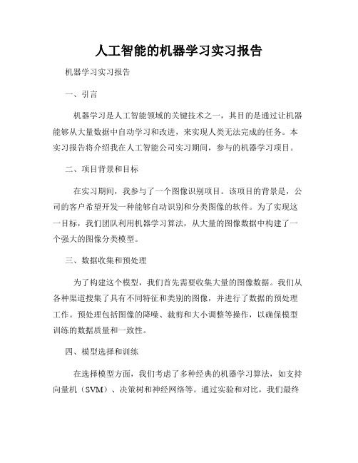
402
132
识别正确率
73.36
84.87
99.71
70.31
82.89
86.84
结果分析:
实验中图像3的识别率最高,图像1和图像2的识别率次之。图像1和图像2的分辨率相对图像3更低,同时图像2有折痕影响而图像1则有大量噪声。通过阈值处理能较好的处理掉图像1的噪声和图像2的折痕,从而使得图像1的识别率有所提升,而图像2的识别率变化不大。从而可以得出结论,图像3和图像2识别率不同的原因主要在于图像分辨率,而图像2和图像1识别率的不同则在于噪声干扰。
实验报告
题目
模式识别系列实验——实验一字符识别实验
内容:
1.利用OCR软件对文字图像进行识别,了解图像处理与模式识别的关系。
2.利用OCR软件对文字图像进行识别,理解正确率的概念。
实验要求:
1.利用photoshop等软件对效果不佳的图像进行预处理,以提高OCR识别的正确率。
2.用OCR软件对未经预处理和经过预处理的简体和繁体中文字符图像进行识别并比较正确率。
图像4内容既有简体又有繁体,从识别结果中可了解到错误基本处在繁体字。
遇到的问题及解决方案:
实验中自动旋转几乎没效果,所以都是采用手动旋转;在对图像4进行识别时若采用系统自己的版面分析,则几乎识别不出什么,所以实验中使用手动画框将诗的内容和标题及作者分开识别。
主要实验方法:
1.使用汉王OCR软件对所给简体和繁体测试文件进行识别;
2.理,再次识别;
实验结果:
不经过图像预处理
经过图像预处理
实验图像
图像1
图像2
图像3
图像4
图像1
图像2
字符总数
458
人工智能的机器学习实习报告
人工智能的机器学习实习报告机器学习实习报告一、引言机器学习是人工智能领域的关键技术之一,其目的是通过让机器能够从大量数据中自动学习和改进,来实现人类无法完成的任务。
本实习报告将介绍我在人工智能公司实习期间,参与的机器学习项目。
二、项目背景和目标在实习期间,我参与了一个图像识别项目。
该项目的背景是,公司的客户希望开发一种能够自动识别和分类图像的软件。
为了实现这一目标,我们团队利用机器学习算法,从大量的图像数据中构建了一个强大的图像分类模型。
三、数据收集和预处理为了构建这个模型,我们首先需要收集大量的图像数据。
我们从各种渠道搜集了具有不同特征和类别的图像,并进行了数据的预处理工作。
预处理包括图像的降噪、裁剪和大小调整等操作,以确保模型训练的数据质量和一致性。
四、模型选择和训练在选择模型方面,我们考虑了多种经典的机器学习算法,如支持向量机(SVM)、决策树和神经网络等。
通过实验和对比,我们最终选择了卷积神经网络(CNN)作为我们的模型。
CNN在图像分类方面表现卓越,能够准确地识别不同的图像特征。
在模型训练阶段,我们使用了大量的图像数据作为输入,并将其分为训练集和验证集。
通过多次迭代训练和调整网络参数,我们不断提高模型的准确性和泛化能力。
最终,我们得到了一个优秀的图像分类模型。
五、模型评估和改进为了评估我们的模型,我们使用测试集对其进行了验证和评测。
我们比较了模型的预测结果与真实标签之间的差异,并计算了准确率、召回率和F1值等指标。
通过评估结果,我们发现模型在大部分图像上都表现出色,但在某些特殊场景下存在一定的识别误差。
针对这些问题,我们对模型进行了改进和优化。
我们尝试了增加训练数据、调整网络结构、改进数据预处理等方法,以进一步提高模型的性能。
经过数次迭代和改进,我们成功降低了模型的误差率,准确度得到了显著提升。
六、实际应用和展望在项目结束后,我们将开发的图像识别系统应用于客户的实际场景中。
通过与客户的合作和反馈,我们不断改进和优化系统,以满足客户的需求。
模式识别实验报告(一二)

信息与通信工程学院模式识别实验报告班级:姓名:学号:日期:2011年12月实验一、Bayes 分类器设计一、实验目的:1.对模式识别有一个初步的理解2.能够根据自己的设计对贝叶斯决策理论算法有一个深刻地认识3.理解二类分类器的设计原理二、实验条件:matlab 软件三、实验原理:最小风险贝叶斯决策可按下列步骤进行: 1)在已知)(i P ω,)(i X P ω,i=1,…,c 及给出待识别的X 的情况下,根据贝叶斯公式计算出后验概率:∑==cj iii i i P X P P X P X P 1)()()()()(ωωωωω j=1,…,x2)利用计算出的后验概率及决策表,按下面的公式计算出采取ia ,i=1,…,a 的条件风险∑==cj j jii X P a X a R 1)(),()(ωωλ,i=1,2,…,a3)对(2)中得到的a 个条件风险值)(X a R i ,i=1,…,a 进行比较,找出使其条件风险最小的决策ka ,即()()1,min k i i aR a x R a x ==则ka 就是最小风险贝叶斯决策。
四、实验内容假定某个局部区域细胞识别中正常(1ω)和非正常(2ω)两类先验概率分别为 正常状态:P (1ω)=; 异常状态:P (2ω)=。
现有一系列待观察的细胞,其观察值为x :已知先验概率是的曲线如下图:)|(1ωx p )|(2ωx p 类条件概率分布正态分布分别为(-2,)(2,4)试对观察的结果进行分类。
五、实验步骤:1.用matlab 完成分类器的设计,说明文字程序相应语句,子程序有调用过程。
2.根据例子画出后验概率的分布曲线以及分类的结果示意图。
3.最小风险贝叶斯决策,决策表如下:结果,并比较两个结果。
六、实验代码1.最小错误率贝叶斯决策 x=[] pw1=; pw2=; e1=-2; a1=; e2=2;a2=2;m=numel(x); %得到待测细胞个数pw1_x=zeros(1,m); %存放对w1的后验概率矩阵 pw2_x=zeros(1,m); %存放对w2的后验概率矩阵results=zeros(1,m); %存放比较结果矩阵for i = 1:m%计算在w1下的后验概率pw1_x(i)=(pw1*normpdf(x(i),e1,a1))/(pw1*normpdf(x(i),e1,a1)+pw2*normp df(x(i),e2,a2)) ;%计算在w2下的后验概率pw2_x(i)=(pw2*normpdf(x(i),e2,a2))/(pw1*normpdf(x(i),e1,a1)+pw2*normp df(x(i),e2,a2)) ;endfor i = 1:mif pw1_x(i)>pw2_x(i) %比较两类后验概率result(i)=0; %正常细胞elseresult(i)=1; %异常细胞endenda=[-5::5]; %取样本点以画图n=numel(a);pw1_plot=zeros(1,n);pw2_plot=zeros(1,n);for j=1:npw1_plot(j)=(pw1*normpdf(a(j),e1,a1))/(pw1*normpdf(a(j),e1,a1)+pw2*no rmpdf(a(j),e2,a2));%计算每个样本点对w1的后验概率以画图pw2_plot(j)=(pw2*normpdf(a(j),e2,a2))/(pw1*normpdf(a(j),e1,a1)+pw2*no rmpdf(a(j),e2,a2));endfigure(1);hold onplot(a,pw1_plot,'co',a,pw2_plot,'r-.');for k=1:mif result(k)==0plot(x(k),,'cp'); %正常细胞用五角星表示elseplot(x(k),,'r*'); %异常细胞用*表示end;end;legend('正常细胞后验概率曲线','异常细胞后验概率曲线','正常细胞','异常细胞');xlabel('样本细胞的观察值');ylabel('后验概率');title('后验概率分布曲线');grid onreturn%实验内容仿真:x = [, ,,, , ,, , , ,,,,,,, ,,,,,,, ]disp(x);pw1=;pw2=;[result]=bayes(x,pw1,pw2);2.最小风险贝叶斯决策x=[]pw1=; pw2=;m=numel(x); %得到待测细胞个数R1_x=zeros(1,m); %存放把样本X判为正常细胞所造成的整体损失R2_x=zeros(1,m); %存放把样本X判为异常细胞所造成的整体损失result=zeros(1,m); %存放比较结果e1=-2;a1=;e2=2;a2=2;%类条件概率分布px_w1:(-2,) px_w2(2,4)r11=0;r12=2;r21=4;r22=0;%风险决策表for i=1:m%计算两类风险值R1_x(i)=r11*pw1*normpdf(x(i),e1,a1)/(pw1*normpdf(x(i),e1,a1)+pw2*norm pdf(x(i),e2,a2))+r21*pw2*normpdf(x(i),e2,a2)/(pw1*normpdf(x(i),e1,a1) +pw2*normpdf(x(i),e2,a2));R2_x(i)=r12*pw1*normpdf(x(i),e1,a1)/(pw1*normpdf(x(i),e1,a1)+pw2*norm pdf(x(i),e2,a2))+r22*pw2*normpdf(x(i),e2,a2)/(pw1*normpdf(x(i),e1,a1) +pw2*normpdf(x(i),e2,a2));endfor i=1:mif R2_x(i)>R1_x(i) %第二类比第一类风险大result(i)=0; %判为正常细胞(损失较小),用0表示elseresult(i)=1; %判为异常细胞,用1表示endenda=[-5::5] ; %取样本点以画图n=numel(a);R1_plot=zeros(1,n);R2_plot=zeros(1,n);for j=1:nR1_plot(j)=r11*pw1*normpdf(a(j),e1,a1)/(pw1*normpdf(a(j),e1,a1)+pw2*n ormpdf(a(j),e2,a2))+r21*pw2*normpdf(a(j),e2,a2)/(pw1*normpdf(a(j),e1, a1)+pw2*normpdf(a(j),e2,a2))R2_plot(j)=r12*pw1*normpdf(a(j),e1,a1)/(pw1*normpdf(a(j),e1,a1)+pw2*n ormpdf(a(j),e2,a2))+r22*pw2*normpdf(a(j),e2,a2)/(pw1*normpdf(a(j),e1, a1)+pw2*normpdf(a(j),e2,a2))%计算各样本点的风险以画图endfigure(1);hold onplot(a,R1_plot,'co',a,R2_plot,'r-.');for k=1:mif result(k)==0plot(x(k),,'cp');%正常细胞用五角星表示elseplot(x(k),,'r*');%异常细胞用*表示end;end;legend('正常细胞','异常细胞','Location','Best');xlabel('细胞分类结果');ylabel('条件风险');title('风险判决曲线');grid onreturn%实验内容仿真:x = [, ,,, , ,, , , ,,,,,,, ,,,,,,, ]disp(x);pw1=;pw2=;[result]=bayes(x,pw1,pw2);七、实验结果1.最小错误率贝叶斯决策后验概率曲线与判决显示在上图中后验概率曲线:带红色虚线曲线是判决为异常细胞的后验概率曲线青色实线曲线是为判为正常细胞的后验概率曲线根据最小错误概率准则,判决结果显示在曲线下方:五角星代表判决为正常细胞,*号代表异常细胞各细胞分类结果(0为判成正常细胞,1为判成异常细胞):0 0 0 0 0 0 0 0 0 0 0 0 0 1 0 1 1 1 0 0 0 1 0 12. 最小风险贝叶斯决策风险判决曲线如上图所示:带红色虚线曲线是异常细胞的条件风险曲线;青色圆圈曲线是正常细胞的条件风险曲线根据贝叶斯最小风险判决准则,判决结果显示在曲线下方:五角星代表判决为正常细胞,*号代表异常细胞各细胞分类结果(0为判成正常细胞,1为判成异常细胞):1 0 0 0 0 0 0 0 0 0 0 0 1 1 0 1 1 1 0 0 0 1 0 1八、实验分析由最小错误率的贝叶斯判决和基于最小风险的贝叶斯判决得出的图形中的分类结果可看出,样本、在前者中被分为“正常细胞”,在后者中被分为“异常细胞”,分类结果完全相反。
人工智能与机器学习实习报告
人工智能与机器学习实习报告1. 引言在当今数字化时代,人工智能(Artificial Intelligence,简称AI)和机器学习(Machine Learning)技术正日益成为各行各业的关键支撑。
本报告旨在总结我在人工智能与机器学习实习中所学到的知识和经验,包括相关概念、应用案例以及实践项目。
2. 人工智能概述人工智能指的是让机器能够模仿和执行类似人类智能的任务。
它可以通过机器学习技术不断学习和优化,从而提供更加智能化的解决方案。
人工智能在图像识别、语音识别、自然语言处理等领域展现出巨大的应用潜力。
3. 机器学习基础机器学习是人工智能的核心技术之一,其通过训练模型使机器能够从数据中学习并做出预测或决策。
常见的机器学习算法包括监督学习、无监督学习和强化学习。
监督学习通过训练数据集中的标签信息来进行学习,而无监督学习则是从无标签的数据中自动发现模式和结构。
4. 人工智能与机器学习应用案例4.1 图像识别技术在人工智能中的应用图像识别技术通过分析和识别图像中的特征来实现自动识别,广泛应用于人脸识别、物体检测、图像检索等领域。
人脸识别技术在安全监控、身份认证等场景中得到广泛应用,物体检测和图像检索技术在电商、医疗等领域也发挥了重要作用。
4.2 语音识别技术在人工智能中的应用语音识别技术通过将声音转化为可理解的文本或命令,实现人机交互的无缝衔接。
它广泛应用于智能助理、智能家居、手机语音输入等领域。
语音助手如Siri、小爱同学等已经成为现代人们生活中不可或缺的一部分。
4.3 自然语言处理技术在人工智能中的应用自然语言处理技术通过对人类语言进行分析和处理,使计算机能够理解和生成自然语言。
它在搜索引擎、智能客服、机器翻译等领域有广泛应用。
自然语言处理的发展为人们提供了更加便捷和高效的信息交流方式。
5. 人工智能与机器学习实践项目在实习期间,我参与了一个基于机器学习的智能推荐系统项目。
通过对用户历史行为数据的分析和建模,我们提供了个性化的推荐服务,帮助用户发现他们可能感兴趣的内容。
模式识别与智能信息处理实践实验报告

模式识别与智能信息处理实践实验报告
一、实验目的
本次实验的目的是:实现基于Matlab的模式识别与智能信息处理。
二、实验内容
1.对实验图片进行处理
根据实验要求,我们选取了两张图片,一张是原始图片,一张是锐化处理后的图片。
使用Matlab的imtool命令进行处理,实现对图片锐化、模糊处理、边缘检测、图像增强等功能。
2.基于模式识别算法进行图像分类
通过Matlab的k-means算法和PCA算法对实验图片进行图像分类,实现对图像数据特征提取,并将图像分类结果可视化。
3.使用智能信息处理技术处理实验数据
使用Matlab的BP网络算法,对实验图片进行处理,并实现实验数据的智能信息处理,以获得准确的分类结果。
三、实验结果
1.图片处理结果
2.图像分类结果
3.智能信息处理结果
四、总结
本次实验中,我们利用Matlab进行模式识别与智能信息处理的实践,实现了对图片的处理,图像分类,以及智能信息处理,从而获得准确的分
类结果。
《模式识别》实验报告-贝叶斯分类
《模式识别》实验报告-贝叶斯分类一、实验目的通过使用贝叶斯分类算法,实现对数据集中的样本进行分类的准确率评估,熟悉并掌握贝叶斯分类算法的实现过程,以及对结果的解释。
二、实验原理1.先验概率先验概率指在不考虑其他变量的情况下,某个事件的概率分布。
在贝叶斯分类中,需要先知道每个类别的先验概率,例如:A类占总样本的40%,B类占总样本的60%。
2.条件概率后验概率指在已知先验概率和条件概率下,某个事件发生的概率分布。
在贝叶斯分类中,需要计算每个样本在各特征值下的后验概率,即属于某个类别的概率。
4.贝叶斯公式贝叶斯公式就是计算后验概率的公式,它是由条件概率和先验概率推导而来的。
5.贝叶斯分类器贝叶斯分类器是一种基于贝叶斯定理实现的分类器,可以用于在多个类别的情况下分类,是一种常用的分类方法。
具体实现过程为:首先,使用训练数据计算各个类别的先验概率和各特征值下的条件概率。
然后,将测试数据的各特征值代入条件概率公式中,计算出各个类别的后验概率。
最后,取后验概率最大的类别作为测试数据的分类结果。
三、实验步骤1.数据集准备本次实验使用的是Iris数据集,数据包含150个Iris鸢尾花的样本,分为三个类别:Setosa、Versicolour和Virginica,每个样本有四个特征值:花萼长度、花萼宽度、花瓣长度、花瓣宽度。
2.数据集划分将数据集按7:3的比例分为训练集和测试集,其中训练集共105个样本,测试集共45个样本。
计算三个类别的先验概率,即Setosa、Versicolour和Virginica类别在训练集中出现的频率。
对于每个特征值,根据训练集中每个类别所占的样本数量,计算每个类别在该特征值下出现的频率,作为条件概率。
5.测试数据分类将测试集中的每个样本的四个特征值代入条件概率公式中,计算出各个类别的后验概率,最后将后验概率最大的类别作为该测试样本的分类结果。
6.分类结果评估将测试集分类结果与实际类别进行比较,计算分类准确率和混淆矩阵。
模式识别实验报告1_简单线性分类实验_实验报告(例)
二、实验环境、内容和方法
环境:windows XP,matlab R2007a
内容:有两类样本(如鲈鱼和鲑鱼),每个样本有两个特征(如长度和亮度),每类有若干个(比如20个)样本点,假设每类样本点服从二维正态分布,自己随机给出具体数据,计算每类数据的均值点,并且把两个均值点连成一线段,用垂直平分该线段的直线作为分类边界。再根据该分类边界对一随机给出的样本判别类别。并画出相应的图形。
方法:线性分类器
三、实验过程描述
1.首先用正态分布normrnd产生两类样本,每类样本两个特征。用不同的均值(ax,ay)=(18,8),(bx,by)=(12,20)。并画出两类样本点。
2.然后,求判别分界线y=k*x+b中的k,b的值。分界线垂直于两类样本的均值点的连线。K,b的值分别为:
k=-(bx-ax)/(by-ay)
y2(:,1) = normrnd(by,6,1,20);
%分解线为y=k*x+b
k=-(bx-ax)/(by-ay);%计算类样本均值连线垂直平分线的斜率k
b=(ay+by)/2+(bx^2-ax^2)/(2*by-2*ay);%计算b的值
figure;%画点
plot(x1,y1,'om',...
实验报告(例子)
课程名称:模式识别实验名称:简单线性分类
提交时间:
专业:计算机应用技术年级:2009级姓名:
一、实验目的和要求
目的:设计简单的线性分类器,了解模式识别的基本方法。
要求:
1.产生两类样本,每类样本两个特征。
2.计算每类数据的均值点,并且把两个均值点连成一线段,用垂直平分该线段的直线作为分类边界。
模式识别实验报告
模式识别实验报告关键信息项:1、实验目的2、实验方法3、实验数据4、实验结果5、结果分析6、误差分析7、改进措施8、结论1、实验目的11 阐述进行模式识别实验的总体目标和期望达成的结果。
111 明确实验旨在解决的具体问题或挑战。
112 说明实验对于相关领域研究或实际应用的意义。
2、实验方法21 描述所采用的模式识别算法和技术。
211 解释选择这些方法的原因和依据。
212 详细说明实验的设计和流程,包括数据采集、预处理、特征提取、模型训练和测试等环节。
3、实验数据31 介绍实验所使用的数据来源和类型。
311 说明数据的规模和特征。
312 阐述对数据进行的预处理操作,如清洗、归一化等。
4、实验结果41 呈现实验得到的主要结果,包括准确率、召回率、F1 值等性能指标。
411 展示模型在不同数据集或测试条件下的表现。
412 提供可视化的结果,如图表、图像等,以便更直观地理解实验效果。
5、结果分析51 对实验结果进行深入分析和讨论。
511 比较不同实验条件下的结果差异,并解释其原因。
512 分析模型的优点和局限性,探讨可能的改进方向。
6、误差分析61 研究实验中出现的误差和错误分类情况。
611 分析误差产生的原因,如数据噪声、特征不充分、模型复杂度不足等。
612 提出减少误差的方法和建议。
7、改进措施71 根据实验结果和分析,提出针对模型和实验方法的改进措施。
711 描述如何优化特征提取、调整模型参数、增加训练数据等。
712 预测改进后的可能效果和潜在影响。
8、结论81 总结实验的主要发现和成果。
811 强调实验对于模式识别领域的贡献和价值。
812 对未来的研究方向和进一步工作提出展望。
在整个实验报告协议中,应确保各项内容的准确性、完整性和逻辑性,以便为模式识别研究提供有价值的参考和借鉴。
机器学习实验报告完整
机器学习实验报告完整摘要:本实验报告旨在探究机器学习算法在数据集上的表现,并评估不同算法的性能。
我们使用了一个包含许多特征的数据集,通过对数据进行预处理和特征选择,进行了多个分类器的比较实验。
实验结果显示,不同的机器学习算法在不同数据集上的表现存在差异,但在对数据进行适当预处理的情况下,性能可以有所改善。
引言:机器学习是一种通过计算机程序来自动学习并改善性能的算法。
机器学习广泛应用于各个领域,例如医学、金融和图像处理等。
在本实验中,我们比较了常用的机器学习算法,并评估了它们在一个数据集上的分类性能。
方法:1. 数据集我们使用了一个包含1000个样本和20个特征的数据集。
该数据集用于二元分类任务,其中每个样本被标记为正类(1)或负类(0)。
2. 预处理在进行实验之前,我们对数据集进行了预处理。
预处理的步骤包括缺失值填充、异常值处理和数据归一化等。
缺失值填充使用常用的方法,例如均值或中位数填充。
异常值处理采用了离群点检测算法,将异常值替换为合理的值。
最后,我们对数据进行了归一化处理,以确保不同特征的尺度一致。
3. 特征选择为了提高分类性能,我们进行了特征选择。
特征选择的目标是从原始特征中选择出最相关的特征子集。
我们使用了常见的特征选择方法,如相关性分析和特征重要性排序。
通过这些方法,我们选取了最具判别能力的特征子集。
4. 算法比较在本实验中,我们选择了四种常见的机器学习算法进行比较:决策树、逻辑回归、支持向量机(SVM)和随机森林。
我们使用Python编程语言中的机器学习库进行实验,分别训练了这些算法,并使用交叉验证进行评估。
评估指标包括准确率、召回率、F1值和ROC曲线下方的面积(AUC)。
结果与讨论:通过对比不同算法在数据集上的性能,我们得出以下结论:1. 决策树算法在本实验中表现欠佳,可能是由于过拟合的原因。
决策树算法可以生成高度解释性的模型,但在处理复杂数据时容易陷入过拟合的状态。
2. 逻辑回归算法表现较好,在数据集上获得了较高的准确率和F1值。
模式识别学习报告(团队)
模式识别学习报告(团队)
简介
本报告是我们团队就模式识别研究所做的总结和讨论。
模式识别是一门关于如何从已知数据中提取信息并作出决策的学科。
在研究过程中,我们通过研究各种算法和技术,了解到模式识别在人工智能、机器研究等领域中的重要性并进行实践操作。
研究过程
在研究过程中,我们首先了解了模式识别的基本概念和算法,如KNN算法、朴素贝叶斯算法、决策树等。
然后我们深入研究了SVM算法和神经网络算法,掌握了它们的实现和应用场景。
在实践中,我们使用了Python编程语言和机器研究相关的第三方库,比如Scikit-learn等。
研究收获
通过研究,我们深刻认识到模式识别在人工智能、机器研究领域中的重要性,了解到各种算法和技术的应用场景和优缺点。
同时我们也发现,在实践中,数据的质量决定了模型的好坏,因此我们需要花费更多的时间来处理数据方面的问题。
团队讨论
在研究中,我们也进行了很多的团队讨论和交流。
一方面,我们优化了研究方式和效率,让研究更加有效率;另一方面我们还就机器研究的基本概念和算法的前沿发展进行了讨论,并提出了一些有趣的问题和方向。
总结
通过学习和团队讨论,我们深刻认识到了模式识别在人工智能和机器学习领域中的核心地位,并获得了实践经验和丰富的团队协作经验。
我们相信这些学习收获和经验会在今后的学习和工作中得到很好的应用。
- 1、下载文档前请自行甄别文档内容的完整性,平台不提供额外的编辑、内容补充、找答案等附加服务。
- 2、"仅部分预览"的文档,不可在线预览部分如存在完整性等问题,可反馈申请退款(可完整预览的文档不适用该条件!)。
- 3、如文档侵犯您的权益,请联系客服反馈,我们会尽快为您处理(人工客服工作时间:9:00-18:30)。
中南大学模式识别与机器学习实验报告班级计科1203 学号 0909121405 姓名雷亦恺指导老师梁毅雄Programming Exercise 1: Linear RegressionIntroductionIn this exercise, you will implement linear regression and get to see it work on data.Before starting on this programming exercise, we strongly recommend watching the video lectures and completing the review questions for the associated topics. To get started with the exercise, you will need to download the starter code and unzip its contents to the directory where you wish to complete the exercise.If needed, use the cd command in Octave to change to this directory before starting this exercise.You can also find instructions for installing Octave on the \Octave Installation" page on the course website.Files included in this exerciseex1.m - Octave script that will help step you through the exerciseex1 multi.m - Octave script for the later parts of the exerciseex1data1.txt - Dataset for linear regression with one variableex1data2.txt - Dataset for linear regression with multiple variablessubmit.m - Submission script that sends your solutions to our servers[*] warmUpExercise.m - Simple example function in Octave[*] plotData.m - Function to display the dataset[*] computeCost.m - Function to compute the cost of linear regression[*] gradientDescent.m - Function to run gradient descent[$] computeCostMulti.m - Cost function for multiple variables[$] gradientDescentMulti.m - Gradient descent for multiple variables[$] featureNormalize.m - Function to normalize features[$] normalEqn.m - Function to compute the normal equations* indicates les you will need to complete$ indicates extra credit exercisesThroughout the exercise, you will be using the scripts ex1.m and ex1 multi.m. These scripts set up the dataset for the problems and make calls to functions that you will write. You do not need to modify either of them.You are only required to modify functions in other les, by following the instructions in this assignment.For this programming exercise, you are only required to complete the rst part of the exercise to implement linear regression with one variable.The second part of the exercise, which you may complete for extra credit, coverslinear regression with multiple variables.根据实验内容补全代码后如下:(1)computeCost.mfunction J = computeCost(X, y, theta)%COMPUTECOST Compute cost for linear regression% J = COMPUTECOST(X, y, theta) computes the cost of using theta as the% parameter for linear regression to fit the data points in X and y% Initialize some useful valuesm = length(y); % number of training examples% You need to return the following variables correctlyJ = 0;% ====================== YOUR CODE HERE ====================== % Instructions: Compute the cost of a particular choice of theta% You should set J to the cost.res = X*theta - y;J = (res’ * res) / m*0.5;%============================================================== ===========end(2)plotData.mfunction plotData(x, y)%PLOTDATA Plots the data points x and y into a new figure% PLOTDATA(x,y) plots the data points and gives the figure axes labels of% population and profit.% ====================== YOUR CODE HERE ====================== % Instructions: Plot the training data into a figure using the% "figure" and "plot" commands. Set the axes labels using% the "xlabel" and "ylabel" commands. Assume the% population and revenue data have been passed in% as the x and y arguments of this function.%% Hint: You can use the 'rx' option with plot to have the markers% appear as red crosses. Furthermore, you can make the% markers larger by using plot(..., 'rx', 'MarkerSize', 10);figure; % open a new figure windowplot(x,y,’rx’,’MarkerSize’,10);xlabel(‘profit in $10,000s’);ylabel(‘Population of City in 10,0000s’);% ============================================================end(3)warmUpExercise.mfunction A = warmUpExercise()%WARMUPEXERCISE Example function in octave% A = WARMUPEXERCISE() is an example function that returns the 5x5 identity matrixA = [];% ============= YOUR CODE HERE ==============% Instructions: Return the 5x5 identity matrix% In octave, we return values by defining which variables% represent the return values (at the top of the file)% and then set them accordingly.A=eye(5);% ===========================================end(4)featureNormalize.mfunction [X_norm, mu, sigma] = featureNormalize(X)%FEATURENORMALIZE Normalizes the features in X% FEATURENORMALIZE(X) returns a normalized version of X where% the mean value of each feature is 0 and the standard deviation% is 1. This is often a good preprocessing step to do when% working with learning algorithms.% You need to set these values correctlyX_norm = X;mu = zeros(1, size(X, 2));sigma = zeros(1, size(X, 2));% ====================== YOUR CODE HERE ====================== % Instructions: First, for each feature dimension, compute the mean% of the feature and subtract it from the dataset,% storing the mean value in mu. Next, compute the% standard deviation of each feature and divide% each feature by it's standard deviation, storing% the standard deviation in sigma.%% Note that X is a matrix where each column is a% feature and each row is an example. You need% to perform the normalization separately for% each feature.%% Hint: You might find the 'mean' and 'std' functions useful.%mu = mean(X_norm);sigma = std(X_norm);X_norm = (X_norm - repmat(mu, size(X,1), 1)) ./repmat(sigma , size(X, 1), 1);% ============================================================ end(5)computeCostMulti.mfunction J = computeCostMulti(X, y, theta)%COMPUTECOSTMULTI Compute cost for linear regression with multiple variables% J = COMPUTECOSTMULTI(X, y, theta) computes the cost of using theta as the% parameter for linear regression to fit the data points in X and y% Initialize some useful valuesm = length(y); % number of training examples% You need to return the following variables correctlyJ = 0;% ====================== YOUR CODE HERE ====================== % Instructions: Compute the cost of a particular choice of theta% You should set J to the cost.res = X*theta - y;J = (res’ * res ) /m *0.5;%============================================================== ===========End(6)gradientDescent.mfunction [theta, J_history] = gradientDescent(X, y, theta, alpha, num_iters)%GRADIENTDESCENT Performs gradient descent to learn theta% theta = GRADIENTDESENT(X, y, theta, alpha, num_iters) updates theta by % taking num_iters gradient steps with learning rate alpha% Initialize some useful valuesm = length(y); % number of training examplesJ_history = zeros(num_iters, 1);for iter = 1:num_iters% ====================== YOUR CODE HERE ======================% Instructions: Perform a single gradient step on the parameter vector% theta.%% Hint: While debugging, it can be useful to print out the values% of the cost function (computeCost) and gradient here.%theta =theta - alpha / m *((X*theta - y))’* X)’;%============================================================ % Save the cost J in every iterationJ_history(iter) = computeCost(X, y, theta);endend(7)gradientDescentMulti.mfunction [theta, J_history] = gradientDescentMulti(X, y, theta, alpha, num_iters) %GRADIENTDESCENTMULTI Performs gradient descent to learn theta% theta = GRADIENTDESCENTMULTI(x, y, theta, alpha, num_iters) updates theta by% taking num_iters gradient steps with learning rate alpha% Initialize some useful valuesm = length(y); % number of training examplesJ_history = zeros(num_iters, 1);for iter = 1:num_iters% ====================== YOUR CODE HERE ======================% Instructions: Perform a single gradient step on the parameter vector% theta.%% Hint: While debugging, it can be useful to print out the values% of the cost function (computeCostMulti) and gradient here.%t = ((X*theta - y)’ *X);theta = theta - alpha /m * t;%============================================================ % Save the cost J in every iterationJ_history(iter) = computeCostMulti(X, y, theta);endend(8)normalEqn.mfunction [theta] = normalEqn(X, y)%NORMALEQN Computes the closed-form solution to linear regression% NORMALEQN(X,y) computes the closed-form solution to linear% regression using the normal equations.theta = zeros(size(X, 2), 1);% ====================== YOUR CODE HERE ====================== % Instructions: Complete the code to compute the closed form solution% to linear regression and put the result in theta.%theta = pinv(X’ *X)*X’ *y;% ---------------------- Sample Solution ----------------------% -------------------------------------------------------------% ============================================================ end总体运行结果如图所示:Programming Exercise 2: Logistic RegressionIntroductionIn this exercise, you will implement logistic regression and apply it to two different datasets. Before starting on the programming exercise, we strongly recommend watching the video lectures and completing the review questions for the associated topics.To get started with the exercise, you will need to download the starter code and unzip its contents to the directory where you wish to complete the exercise. If needed, use the cd command in Octave to change to this directory before starting this exercise.You can also find instructions for installing Octave on the \Octave Installation" page on the course website.Files included in this exerciseex2.m - Octave script that will help step you through the exerciseex2 reg.m - Octave script for the later parts of the exerciseex2data1.txt - Training set for the rst half of the exerciseex2data2.txt - Training set for the second half of the exercisesubmitWeb.m - Alternative submission scriptsubmit.m - Submission script that sends your solutions to our servers mapFeature.m - Function to generate polynomial features plotDecisionBounday.m - Function to plot classier's decision boundary[*] plotData.m - Function to plot 2D classication data[*] sigmoid.m - Sigmoid Function[*] costFunction.m - Logistic Regression Cost Function[*] predict.m - Logistic Regression Prediction Function[*] costFunctionReg.m - Regularized Logistic Regression Cost* indicates les you will need to completeThroughout the exercise, you will be using the scripts ex2.m and ex2 reg.m. These scripts set up the dataset for the problems and make calls to functions that you will write. You do not need to modify either of them. You are only required to modify functions in other les, by following the instructions inthis assignment.根据实验内容补全代码后如下:(1)plotData.mfunction plotData(X, y)%PLOTDATA Plots the data points X and y into a new figure% PLOTDATA(x,y) plots the data points with + for the positive examples% and o for the negative examples. X is assumed to be a Mx2 matrix.% Create New Figurefigure; hold on;% ====================== YOUR CODE HERE ====================== % Instructions: Plot the positive and negative examples on a% 2D plot, using the option 'k+' for the positive% examples and 'ko' for the negative examples.%positive = find (y == 1);negative = find (y==0);plot (X(positive, 1), X(positive,2), ‘k+’, ‘MarkerSize’, 7 ,’LineWidth’,2);plot (X(negative, 1), X(negative,2), ‘ko’, ‘MarkerFaceColor’, ‘y’ ,’MarkSize’,7);%============================================================== ===========hold off;end(2)Sigmoid.mfunction g = sigmoid(z)%SIGMOID Compute sigmoid functoon% J = SIGMOID(z) computes the sigmoid of z.% You need to return the following variables correctlyg = zeros(size(z));% ====================== YOUR CODE HERE ====================== % Instructions: Compute the sigmoid of each value of z (z can be a matrix,% vector or scalar).g = 1./(1+exp(-z));%=============================================================end(3)costFunction.mfunction [J, grad] = costFunction(theta, X, y)%COSTFUNCTION Compute cost and gradient for logistic regression% J = COSTFUNCTION(theta, X, y) computes the cost of using theta as the% parameter for logistic regression and the gradient of the cost% w.r.t. to the parameters.% Initialize some useful valuesm = length(y); % number of training examples% You need to return the following variables correctlyJ = 0;grad = zeros(size(theta));% ====================== YOUR CODE HERE ====================== % Instructions: Compute the cost of a particular choice of theta.% You should set J to the cost.% Compute the partial derivatives and set grad to the partial % derivatives of the cost w.r.t. each parameter in theta%Hypothesis = sigmoid (X*theta);J=1/m*sum(-y.*log(hypothesis)-(1-y).*log(1-hypothesis))+0.5*lambda/m*(theta (2:end)’*theta(2:end));n = size(X,2);grad(1) = 1/m*dot(hypothesis-y,X(:,1));for i =2 : ngrad(i) = 1/m*dot(hypothesis - y,X(:,i))+lambda /m * theta(i);% Note: grad should have the same dimensions as theta%%=============================================================end(4)Predict.mfunction p = predict(theta, X)%PREDICT Predict whether the label is 0 or 1 using learned logistic%regression parameters theta% p = PREDICT(theta, X) computes the predictions for X using a% threshold at 0.5 (i.e., if sigmoid(theta'*x) >= 0.5, predict 1)m = size(X, 1); % Number of training examples% You need to return the following variables correctlyp = zeros(m, 1);% ====================== YOUR CODE HERE ====================== % Instructions: Complete the following code to make predictions using% your learned logistic regression parameters.% You should set p to a vector of 0's and 1's%p= sigmoid(X*theta) >= 0.5;%============================================================== ===========end(5)costFunctionReg.mfunction [J, grad] = costFunctionReg(theta, X, y, lambda)%COSTFUNCTIONREG Compute cost and gradient for logistic regression with regularization% J = COSTFUNCTIONREG(theta, X, y, lambda) computes the cost of using% theta as the parameter for regularized logistic regression and the% gradient of the cost w.r.t. to the parameters.% Initialize some useful valuesm = length(y); % number of training examples% You need to return the following variables correctlyJ = 0;grad = zeros(size(theta));% ====================== YOUR CODE HERE ====================== % Instructions: Compute the cost of a particular choice of theta.% You should set J to the cost.% Compute the partial derivatives and set grad to the partial% derivatives of the cost w.r.t. each parameter in theta hypothesis = sigmoid (X*theta);J=1/m*sum(-y.*log(hypothesis)-(1-y).*log(1-hypothesis))+0.5*lambda/m*(theta (2:end)’*theta(2:end));n = size(X,2);grad(1) = 1/m*dot(hypothesis-y,X(:,1));for i =2 : ngrad(i) = 1/m*dot(hypothesis - y,X(:,i))+lambda /m * theta(i);%============================================================= End运行后结果如下:。