Stata软件操作教程(15)
使用Stata进行数据分析的教程
使用Stata进行数据分析的教程第一章:介绍StataStata是一种统计软件,经常被研究人员和学者用于数据分析和统计建模。
它提供了强大的数据处理和分析功能,可以应用于不同领域的研究项目。
本章介绍了Stata的基本功能和特点,包括数据管理、数据操作和Stata的界面等。
1.1 Stata的起源和发展Stata最初是由James Hardin和William Gould创建的,旨在为统计学家和社会科学研究人员提供一个数据分析工具。
随着时间的推移,Stata得到了广泛的应用,并逐渐发展成为一种强大的统计软件。
1.2 Stata的功能和特点Stata提供了许多数据处理和分析函数,包括描述性统计、回归分析、因子分析和生存分析等。
它还具有数据的管理功能,可以导入、导出和编辑数据文件。
Stata的界面友好,并且支持批处理和交互模式。
第二章:数据管理与准备在进行数据分析之前,首先需要准备和管理数据集。
本章将详细介绍Stata中的数据导入、数据清洗和数据变换等操作。
2.1 数据导入与导出Stata可以导入各种格式的数据文件,包括CSV、Excel和SPSS 等。
同时,Stata也支持将分析结果导出为不同的格式,如PDF和HTML等。
2.2 数据清洗和缺失值处理在实际研究中,数据常常存在缺失值和异常值。
Stata提供了处理缺失值和异常值的方法,可以通过删除、替换或插补来处理这些问题。
2.3 数据变换和指标构造数据变换是指将原始数据转化为适合分析的形式,常见的变换包括对数变换、差分和标准化等。
指标构造是指根据已有变量构造新的变量,如计算平均值和构造虚拟变量等。
第三章:描述性统计和数据可视化描述性统计是对数据集的基本统计特征进行总结和分析,而数据可视化则是通过图表和图形展示数据的特征和关系。
本章将介绍在Stata中进行描述性统计和数据可视化的方法。
3.1 中心趋势和离散程度的度量通过计算平均值、中位数和众数等指标来描述数据的中心趋势。
stata入门教程
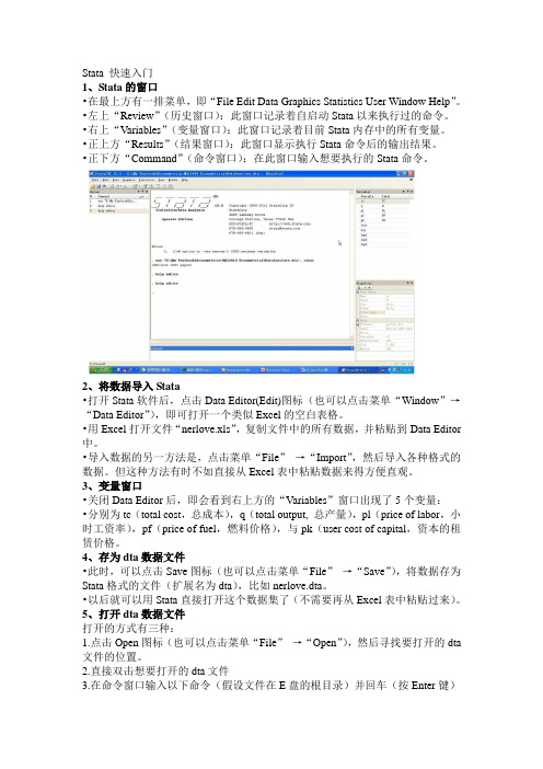
Stata 快速入门1、Stata的窗口•在最上方有一排菜单,即“File Edit Data Graphics Statistics User Window Help”。
•左上“Review”(历史窗口):此窗口记录着自启动Stata以来执行过的命令。
•右上“Variables”(变量窗口):此窗口记录着目前Stata内存中的所有变量。
•正上方“Results”(结果窗口):此窗口显示执行Stata命令后的输出结果。
•正下方“Command”(命令窗口):在此窗口输入想要执行的Stata命令。
2、将数据导入Stata•打开Stata软件后,点击Data Editor(Edit)图标(也可以点击菜单“Window”→“Data Editor”),即可打开一个类似Excel的空白表格。
•用Excel打开文件“nerlove.xls”,复制文件中的所有数据,并粘贴到Data Editor 中。
•导入数据的另一方法是,点击菜单“File”→“Import”,然后导入各种格式的数据。
但这种方法有时不如直接从Excel表中粘贴数据来得方便直观。
3、变量窗口•关闭Data Editor后,即会看到右上方的“Variables”窗口出现了5个变量:•分别为tc(total cost,总成本),q(total output, 总产量),pl(price of labor,小时工资率),pf(price of fuel,燃料价格),与pk(user cost of capital,资本的租赁价格。
4、存为dta数据文件•此时,可以点击Save图标(也可以点击菜单“File”→“Save”),将数据存为Stata格式的文件(扩展名为dta),比如nerlove.dta。
•以后就可以用Stata直接打开这个数据集了(不需要再从Excel表中粘贴过来)。
5、打开dta数据文件打开的方式有三种:1.点击Open图标(也可以点击菜单“File”→“Open”),然后寻找要打开的dta 文件的位置。
stata简明教程

几个简单的例子 di use sysuse sum scatter gen
举例:画出Y=X2的曲线图
drop _all (drop data from memory) set obs 100 (make 100 observations) gen x = _n (x = 1, 2, 3, .., 100) gen y = x^2 (y = 2, 4, 9, .., 10000) scatter y x (make a graph)
命令格式简介
stata命令格式
[by varlist:] command [varlist] [=exp] [if exp] [in range] [weight] [, options]
1。Command 命令动词,经常用缩写。 2。varlist 表示一个变量或者多个变量,多 个变量之间用空格隔开。如 sum price weight
添加标签
打开wage1数据文件。 1。为整个数据添加标签:例如,将数据命名为“工 资表”。
菜单:Data->Labels->Label dataset 命令:label data “工资表“ 2。为变量增加标签,例如,给变量wage增加标签 “年工资总额” 菜单:Data->Labels->Label variables 命令 label variable wage “年工资总额”
summarize---sum describe------des 得到正确命令缩写的简单方法:看help。
几条最简单的命令
use 打开数据文件,一般加clear选型清空 内存中现有数据。 sysuse 打开系统数据文件。 describe 描述数据 edit 利用数据编辑器进行数据编辑 list 类似于edit,但只能显示不能修改数据。
stata入门常用命令
stata入门常用命令Stata是一种统计分析软件,在社会科学、医学等研究领域很常用。
以下是Stata入门常用命令:1.数据加载use "文件路径":加载Stata数据,文件路径为数据文件所在的路径。
describe:显示数据集的变量名、数据类型、缺失值和数据分布等。
2.变量处理generate 变量名=表达式:生成新变量(如指数变量),并可以使用算数、统计和逻辑运算。
replace 变量名=新值:替换某变量中的指定值(如缺失值)为新值。
drop 变量名:删除数据集中的变量。
rename 旧变量名 = 新变量名...:将变量改名。
recode 变量名(包含的值) = 新值:根据变量取值对其离散化。
3.数据子集sort 变量名...:按指定变量排序数据。
by 变量名:...:在一个或多个变量上划分数据集,然后对每个子集应用命令。
if (条件):指定一个条件,只选取满足条件的数据记录。
merge 命令:将两个或多个数据集根据指定变量进行合并。
4.数据汇总summarize:按变量计算数值统计(如平均值、标准差、中位数和四分位数)。
tabulate 变量名:对变量进行交叉分析,并产生表格输出。
5.数据可视化histogram 变量名:绘制直方图。
scatter 变量名1 变量名2:绘制散点图。
graph 命令:绘制多种类型的图表,例如线图和条形图。
6.线性回归regress 因变量自变量1 自变量2...:通过最小二乘法拟合多元线性回归模型。
test 命令:进行t检验、F检验、方差分析等统计检验。
predict 新变量名:计算回归模型的预测值或残差值,并存储在新的变量中。
7.度量方法计算correlate 命令:计算并存储所有变量的相关系数矩阵。
haase 命令:计算哈斯变换矩阵。
Inflate 命令:计算一个变量的方差膨胀因子和条件数。
8.模态分析(模拟)simulate 命令:用随机抽样模拟数据,计算一个或多个变量的特定函数或方程,并存储结果。
Stata软件使用指南说明书

18Learning more about StataWhere to go from hereYou now know plenty enough to use Stata.There is still much,much more to learn because Stata is a rich environment for doing statistical analysis and data management.What should you do to learn more?•Get an interesting dataset and play with Stata.e the menus and dialog system to experiment with commands.Notice what commandsshow up in the Results window.You willfind that Stata’s simple and consistent commandsyntax will make the commands easy to read so that you will know what you have doneand easy to remember so that typing some commands will be faster than using menus.b.Play with graphs and the Graph Editor.•If you venture into the Command window,you willfind that many things will go faster.You will alsofind that it is possible to make mistakes where you cannot understand why Stata is balking.a.Try help commandname or Help>Stata command...and entering the command name.b.Look at the command syntax and the examples in the helpfile,and compare themwith what you pare them closely:small typographical errors make commandsimpossible for Stata to parse.•Explore Stata by selecting Help>Search....You will uncover many statistical routines that could be of great use.•Look through the Combined subject table of contents in the Stata Index.•Read and work your way through the User’s Guide.It is designed to be read from cover to cover,and it contains most of the information you need to become an expert Stata user.It is well worth reading.If you are not this ambitious and instead prefer to sample the User’s Guide and the references,there is some advice later in this chapter for you.•Browse through the reference manuals to read about statistical methods you like to use,making use of the links to jump to other topics.The reference manuals are not meant to be read from cover to cover—they are meant to be referred to as you would an encyclopedia.You canfind the datasets used in the examples in the manuals by selecting File>Example datasets...and then clicking on Stata18manual datasets.Doing so will enable you to work through the examples quickly.•Stata has much information,including answers to frequently asked questions(FAQ s),at https:///support/faqs/.•There are many useful links to Stata resources at https:///links/.Be sure to look at these materials because many outstanding resources about Stata are listed here.•Join Statalist,a forum devoted to discussion of Stata and statistics.•Read The Stata Blog:Not Elsewhere Classified at https:// to read articles written by people at Stata about all things Stata.•Visit Stata on Facebook at https:///statacorp,join Stata on Instagram at https:///statacorp,find Stata on LinkedIn at https:///company/statacorp,and follow Stata on Twitter at https:///stata to keep up with Stata.•Subscribe to the Stata Journal,which contains reviewed papers,regular columns,book reviews, and other material of interest to researchers applying statistics in a variety of disciplines.Visit https://.12[GSM]18Learning more about Stata•Many supplementary books about Stata are available.Visit the Stata Bookstore athttps:///bookstore/.•Take a Stata NetCourse R .NetCourse101is an excellent choice for learning about Stata.See https:///netcourse/for course information and schedules.•Attend a classroom or a web-based training course taught by StataCorp.Visithttps:///training/classroom-and-web/for course information and schedules.•View a webinar led by Stata developers.Visit https:///training/webinar/for the current list of topics and schedule.•Watch Stata videos at https:///user/statacorp.Suggested reading from the User’s Guide and reference manuals The User’s Guide is designed to be read from cover to cover.The reference manuals are designed as references to be sampled when necessary.Ideally,after reading this Getting Started manual,you should read the User’s Guide from cover to cover,but you probably want to become at least somewhat proficient in Stata right away.Here isa suggested reading list of sections from the User’s Guide and the reference manuals to help you onyour way to becoming a Stata expert.This list covers fundamental features and points you to some less obvious features that you might otherwise overlook.Basic elements of Stata[U]11Language syntax[U]12Data[U]13Functions and expressionsData management[U]6Managing memory[U]22Entering and importing data[D]import—Overview of importing data into Stata[D]append—Append datasets[D]merge—Merge datasets[D]compress—Compress data in memory[D]frames intro—Introduction to framesGraphics[G]Stata Graphics Reference ManualReproducible research[U]16Do-files[U]17Ado-files[U]13.5Accessing coefficients and standard errors[U]13.6Accessing results from Stata commands[U]21Creating reports[RPT]Dynamic documents intro—Introduction to dynamic documents[RPT]putdocx intro—Introduction to generating Office Open XML(.docx)files[RPT]putexcel—Export results to an Excelfile[RPT]putpdf intro—Introduction to generating PDFfiles[R]log—Echo copy of session tofile[GSM]18Learning more about Stata3Useful features that you might overlook[U]29Using the Internet to keep up to date[U]19Immediate commands[U]24Working with strings[U]25Working with dates and times[U]26Working with categorical data and factor variables[U]27Overview of Stata estimation commands[U]20Estimation and postestimation commands[R]estimates—Save and manipulate estimation resultsBasic statistics[R]anova—Analysis of variance and covariance[R]ci—Confidence intervals for means,proportions,and variances[R]correlate—Correlations of variables[D]egen—Extensions to generate[R]regress—Linear regression[R]predict—Obtain predictions,residuals,etc.,after estimation[R]regress postestimation—Postestimation tools for regress[R]test—Test linear hypotheses after estimation[R]summarize—Summary statistics[R]table intro—Introduction to tables of frequencies,summaries,and command results [R]tabulate oneway—One-way table of frequencies[R]tabulate twoway—Two-way table of frequencies[R]ttest—t tests(mean-comparison tests)Matrices[U]14Matrix expressions[U]18.5Scalars and matrices[M]Mata Reference ManualProgramming[U]16Do-files[U]17Ado-files[U]18Programming Stata[R]ml—Maximum likelihood estimation[P]Stata Programming Reference Manual[M]Mata Reference ManualSystem values[R]set—Overview of system parameters[P]creturn—Return c-class values4[GSM]18Learning more about StataInternet resourcesThe Stata website(https://)is a good place to get more information about Stata.You willfind answers to FAQ s,ways to interact with other users,official Stata updates,and other useful information.You can also join Statalist,a forum devoted to discussion of Stata and statistics.You will alsofind information on Stata NetCourses R ,which are interactive courses offered over the Internet that vary in length from a few weeks to eight weeks.Stata also offers in-person and web-based training sessions,as well as webinars on Stata features.Visit https:///learn/ for more information.At the website is the Stata Bookstore,which contains books that we feel may be of interest to Stata users.Each book has a brief description written by a member of our technical staff explaining why we think this book may be of interest.We suggest that you take a quick look at the Stata website now.You can register your copy of Stata online and request a free subscription to the Stata News.Visit https:// for information on books,manuals,and journals published by Stata Press.The datasets used in examples in the Stata manuals are available from the Stata Press website.Also visit https:// to read about the Stata Journal,a quarterly publication containing articles about statistics,data analysis,teaching methods,and effective use of Stata’s language.Visit Stata’s official blog at https:// for news and advice related to the use of Stata.The articles appearing in the blog are individually signed and are written by the same people who develop,support,and sell Stata.The Stata Blog:Not Elsewhere Classified also has links to other blogs about Stata,written by Stata users around the world.Follow Stata on Facebook at https:///statacorp,Twitter at https:///stata, Instagram at https:///statacorp,and LinkedIn athttps:///company/statacorp.You may also follow Stata on Twitter athttps:///stata fr or https:///stata es.These are good ways to stay up-to-the-minute with the latest Stata information.Watch short example videos of using Stata on YouTube at https:///user/statacorp.See[GSM]19Updating and extending Stata—Internet functionality for details on accessing official Stata updates and free additions to Stata on the Stata website.[GSM]18Learning more about Stata5 Stata,Stata Press,and Mata are registered trademarks of StataCorp LLC.Stata andStata Press are registered trademarks with the World Intellectual Property Organization®of the United Nations.Other brand and product names are registered trademarks ortrademarks of their respective companies.Copyright c 1985–2023StataCorp LLC,College Station,TX,USA.All rights reserved.。
STATA面板数据模型操作命令讲解
STATA面板数据模型操作命令讲解1. xtset:该命令用于设置面板数据模型的数据结构。
在使用面板数据模型命令之前,需要先使用xtset命令来指定数据集的面板结构。
例如,如果数据集中包含一列代表时间(年份)和一列代表个体(公司),则可以使用以下命令指定数据结构:2. xtreg:该命令用于估计面板数据模型的普通最小二乘回归系数。
以下是xtreg命令的一般形式:xtreg dependent_var independent_vars, options其中,dependent_var是依赖变量,independent_vars是自变量,options是可选参数。
通过指定options参数,可以对估计结果进行调整和控制,例如指定固定效应、随机效应或混合效应模型。
3. xtreg, fe:该命令用于估计固定效应模型。
固定效应模型是一种控制个体固定效应的面板数据模型。
使用以下命令可以估计固定效应模型:xtreg dependent_var independent_vars, fe通过指定fe参数,可以估计固定效应模型,并控制除个体固定效应以外的其他混杂效应。
4. xtreg, re:该命令用于估计随机效应模型。
随机效应模型是一种允许个体固定效应和随机效应的面板数据模型。
使用以下命令可以估计随机效应模型:xtreg dependent_var independent_vars, re通过指定re参数,可以估计随机效应模型,并考虑个体固定效应和随机效应对因变量的影响。
5. xtreg, mle:该命令用于估计混合效应模型。
混合效应模型是一种允许个体固定效应和随机效应的面板数据模型,并且可以对效应参数进行最大似然估计。
使用以下命令可以估计混合效应模型:xtreg dependent_var independent_vars, mle通过指定mle参数,可以估计混合效应模型,并通过最大似然估计法对参数进行估计。
stata操作指南
stata操作指南计量经济学stata操作(实验课)第一章stata基本知识1、stata窗口介绍2、基本操作(1)窗口锁定:Edit-preferences-general preferences-windowing-lock splitter (2)数据导入(3)打开文件:use E:\example.dta,clear(4)日期数据导入:gen newvar=date(varname, “ymd”)format newvar %td 年度数据gen newvar=monthly(varname, “ym”)format newvar %tm 月度数据gen newvar=quarterly(varname, “yq”)format newvar %tq 季度数据(5)变量标签Label variable tc ` “total output” ’(6)审视数据describelist x1 x2list x1 x2 in 1/5list x1 x2 if q>=1000drop if q>=1000keep if q>=1000(6)考察变量的统计特征summarize x1su x1 if q>=10000su q,detailsutabulate x1correlate x1 x2 x3 x4 x5 x6(7)画图histogram x1, width(1000) frequency kdensity x1scatter x1 x2twoway (scatter x1 x2) (lfit x1 x2) twoway (scatter x1 x2) (qfit x1 x2) (8)生成新变量gen lnx1=log(x1)gen q2=q^2gen lnx1lnx2=lnx1*lnx2gen larg=(x1>=10000)rename larg largeg large=(q>=6000)replace large=(q>=6000)drop ln*(8)计算功能display log(2)(9)线性回归分析regress y1 x1 x2 x3 x4vce #显示估计系数的协方差矩阵reg y1 x1 x2 x3 x4,noc #不要常数项reg y1 x1 x2 x3 x4 if q>=6000reg y1 x1 x2 x3 x4 if largereg y1 x1 x2 x3 x4 if large==0reg y1 x1 x2 x3 x4 if ~large predict yhatpredict e1,residualdisplay 1/_b[x1]test x1=1 # F检验,变量x1的系数等于1test (x1=1) (x2+x3+x4=1) # F联合假设检验test x1 x2 #系数显著性的联合检验testnl _b[x1]= _b[x2]^2(10)约束回归constraint def 1 x1+x2+x3=1cnsreg y1 x1 x2 x3 x4,c(1)cons def 2 x4=1cnsreg y1 x1 x2 x3 x4,c(1-2)(11)stata的日志File-log-begin-输入文件名log off 暂时关闭log on 恢复使用log close 彻底退出(12)stata命令库更新Update allhelp command第二章有关大样本ols的stata命令及实例(1)ols估计的稳健标准差reg y x1 x2 x3,robust(2)实例use example.dta,clearreg y1 x1 x2 x3 x4test x1=1reg y1 x1 x2 x3 x4,rtestnl _b[x1]=_b[x2]^2第三章最大似然估计法的stata命令及实例(1)最大似然估计help ml(2)LR检验lrtest #对面板数据中的异方差进行检验(3)正态分布检验sysuse auto #调用系统数据集auto.dtahist mpg,normalkdensity mpg,normalqnorm mpg*手工计算JB统计量sum mpg,detaildi (r(N)/6)*((r(skewness)^2)+[(1/4)*(r(kurtosis)-3)^2]) di chi2tail(自由度,上一步计算值)*下载非官方程序ssc install jb6jb6 mpg*正态分布的三个检验sktest mpgswilk mpgsfrancia mpg*取对数后再检验gen lnmpg=log(mpg)kdensity lnmpg, normaljb6 lnmpgsktest lnmpg第四章处理异方差的stata命令及实例(1)画残差图rvfplotrvfplot varname*例题use example.dta,clearreg y x1 x2 x3 x4rvfplot # 与拟合值的散点图rvfplot x1 # 画残差与解释变量的散点图(2)怀特检验estat imtest,white*下载非官方软件ssc install whitetst(3)BP检验estat hettest #默认设置为使用拟合值estat hettest,rhs #使用方程右边的解释变量estat hettest [varlist] #指定使用某些解释变量estat hettest,iidestat hettest,rhs iidestat hettest [varlist],iid(4)WLSreg y x1 x2 x3 x4 [aw=1/var]*例题quietly reg y x1 x2 x3 x4predict e1,resgen e2=e1^2gen lne2=log(e2)reg lne2 x2,nocpredict lne2fgen e2f=exp(lne2f)reg y x1 x2 x3 x4 [aw=1/e2f](5)stata命令的批处理(写程序)Window-do-file editor-new do-file#WLS for examplelog using E:\wls_example.smcl,replaceset more offuse E:\example.dta,clearreg y x1 x2 x3 x4predict e1,resgen e2=e1^2g lne2=log(e2)reg lne2 x2,nocpredict lne2fg e2f=exp(lne2f)*wls regressionreg y x1 x2 x3 x4 [aw=1/e2f]log closeexit第五章处理自相关的stata命令及实例(1)滞后算子/差分算子tsset yearl.l2.D.D2.LD.(2)画残差图scatter e1 l.e1ac e1pac e1(3)BG检验estat bgodfrey(默认p=1)estat bgodfrey,lags(p)estat bgodfrey,nomiss0(使用不添加0的BG检验)(4)Ljung-Box Q检验reg y x1 x2 x3 x4predict e1,residwntestq e1wntestq e1,lags(p)* wntestq指的是“white noise test Q”,因为白噪声没有自相关(5)DW检验做完OLS回归后,使用estat dwatson(6)HAC稳健标准差newey y x1 x2 x3 x4,lag(p)reg y x1 x2 x3 x4,cluster(varname)(7)处理一阶自相关的FGLSprais y x1 x2 x3 x4 (使用默认的PW估计方法)prais y x1 x2 x3 x4,corc (使用CO估计法)(8)实例use icecream.dta, cleartsset timegraph twoway connect consumption temp100 time, msymbol(circle) msymbol(triangle) reg consumption temp price incomepredict e1, resg e2=l.e1twoway (scatter e1 e2) (lfit e1 e2)ac e1pac e1estat bgodfreywntestq e1estat dwatsonnewey consumption temp price income, lag (3)prais consumption temp price income, corcprais consumption temp price income, nologreg consumption temp l.temp price incomeestat bgodfreyestat dwatson第六章模型设定与数据问题(1)解释变量的选择reg y x1 x2 x3estat ic*例题use icecream.dta, clearreg consumption temp price incomeestat icreg consumption temp l.temp price incomeestat ic(2)对函数形式的检验(reset检验)reg y x1 x2 x3estat ovtest (使用被解释变量的2、3、4次方作为非线性项)estat ovtest, rhs (使用解释变量的幂作为非线性项,ovtest-omitted variable test)*例题use nerlove.dta, clearreg lntc lnq lnpl lnpk lnpfestat ovtestg lnq2=lnq^2reg lntc lnq lnq2 lnpl lnpk lnpfestat ovtest(3)多重共线性estat vif*例题use nerlove.dta, clearreg lntc lnq lnpl lnpk lnpfestat vif(4)极端数据reg y x1 x2 x3predict lev, leverage (列出所有解释变量的lev值)gsort –levsum levlist lev in 1/3*例题use nerlove.dta, clearquietly reg lntc lnq lnpl lnpk lnpfpredict lev, leveragesum levgsort –levlist lev in 1/3(5)虚拟变量gen d=(year>=1978)tabulate province, generate (pr)reg y x1 x2 x3 pr2-pr30(6)经济结构变动的检验方法1:use consumption_china.dta, cleargraph twoway connect c y year, msymbol(circle) msymbol(triangle)reg c yreg c y if year<1992reg c y if year>=1992计算F统计量方法2:gen d=(year>1991)gen yd=y*dreg c y d ydtest d yd第七章工具变量法的stata命令及实例(1)2SLS的stata命令ivregress 2sls depvar [varlist1] (varlist2=instlist)如:ivregress 2sls y x1 (x2=z1 z2)ivregress 2sls y x1 (x2 x3=z1 z2 z3 z4) ,r firstestat firststage,all forcenonrobust (检验弱工具变量的命令)ivregress liml depvar [varlist 1] (varlist2=instlist)estat overid (过度识别检验的命令)*对解释变量内生性的检验(hausman test),缺点:不适合于异方差的情形reg y x1 x2estimates store olsivregress 2sls y x1 (x2=z1 z2)estimates store ivhausman iv ols, constant sigmamore*DWH检验estat endogenous*GMM的过度识别检验ivregress gmm y x1 (x2=z1 z2) (两步GMM)ivregress gmm y x1 (x2=z1 z2),igmm (迭代GMM)estat overid*使用异方差自相关稳健的标准差GMM命令ivregress gmm y x1 (x2=z1 z2), vce (hac nwest[#])(2)实例use grilic.dta,clearsumcorr iq sreg lw s expr tenure rns smsa,rreg lw s iq expr tenure rns smsa,rivregress 2sls lw s expr tenure rns smsa (iq=med kww mrt age),restat overidivregress 2sls lw s expr tenure rns smsa (iq=med kww),r first estat overidestat firststage, all forcenonrobust (检验工具变量与内生变量的相关性)ivregress liml lw s expr tenure rns smsa (iq=med kww),r *内生解释变量检验quietly reg lw s iq expr tenure rns smsaestimates store olsquietly ivregress 2sls lw s expr tenure rns smsa (iq=med kww) estimates store ivhausman iv ols, constant sigmamoreestat endogenous (存在异方差的情形)*存在异方差情形下,GMM比2sls更有效率ivregress gmm lw s expr tenure rns smsa (iq=med kww)estat overidivregress gmm lw s expr tenure rns smsa (iq=med kww),igmm*将各种估计方法的结果存储在一张表中quietly ivregress gmm lw s expr tenure rns smsa (iq=med kww)estimates store gmmquietly ivregress gmm lw s expr tenure rns smsa (iq=med kww),igmmestimates store igmmestimates table gmm igmm第八章短面板的stata命令及实例(1)面板数据的设定xtset panelvar timevarencode country,gen(cntry) (将字符型变量转化为数字型变量)xtdesxtsumxttab varnamextline varname,overlay*实例use traffic.dta,clearxtset state yearxtdesxtsum fatal beertax unrate state yearxtline fatal(2)混合回归reg y x1 x2 x3,vce(cluster id)如:reg fatal beertax unrate perinck,vce(cluster state)estimates store ols对比:reg fatal beertax unrate perinck(3)固定效应xtreg y x1 x2 x3,fe vce(cluster id)xi:reg y x1 x2 x3 i.id,vce(cluster id) (LSDV法)xtserial y x1 x2 x3,output (一阶差分法,同时报告面板一阶自相关)estimates store FD*双向固定效应模型tab year, gen (year)xtreg fatal beertax unrate perinck year2-year7, fe vce (cluster state)estimates store FE_TWtest year2 year3 year4 year5 year6 year7(4)随机效应xtreg y x1 x2 x3,re vce(cluster id) (随机效应FGLS)xtreg y x1 x2 x3,mle (随机效应MLE)xttest0 (在执行命令xtreg, re 后执行,进行LM检验)(5)组间估计量xtreg y x1 x2 x3,be(6)固定效应还是随机效应:hausman testxtreg y x1 x2 x3,feestimates store fextreg y x1 x2 x3,reestimates store rehausman fe re,constant sigmamore (若使用了vce(cluster id),则无法直接使用该命令,解决办法详见P163)estimates table ols fe_robust fe_tw re be, b se (将主要回归结果列表比较)第九章长面板与动态面板(1)仅解决组内自相关的FGLSxtpcse y x1 x2 x3 ,corr(ar1) (具有共同的自相关系数)xtpcse y x1 x2 x3 ,corr(psar1) (允许每个面板个体有自身的相关系数)例题:use mus08cigar.dta,cleartab state,gen(state)gen t=year-62reg lnc lnp lnpmin lny state2-state10 t,vce(cluster state)estimates store OLSxtpcse lnc lnp lnpmin lny state2-state10 t,corr(ar1) (考虑存在组内自相关,且各组回归系数相同)estimates store AR1xtpcse lnc lnp lnpmin lny state2-state10 t,corr(psar1) (考虑存在组内自相关,且各组回归系数不相同)estimates store PSAR1xtpcse lnc lnp lnpmin lny state2-state10 t, hetonly (仅考虑不同个体扰动性存在异方差,忽略自相关)estimates store HETONL Yestimates table OLS AR1 PSAR1 HETONL Y, b se(2)同时处理组内自相关与组间同期相关的FGLSxtgls y x1 x2 x3,panels (option/iid/het/cor) corr(option/ar1/psar1) igls注:执行上述xtpcse、xtgls命令时,如果没有个体虚拟变量,则为随机效应模型;如果加上个体虚拟变量,则为固定效应模型。
STATA简易操作
输入数据 命令 框
单击命令框按键,会出现下面的命令窗口
在窗口中 输入命令, 单击 Execute键, 即可执行 该命令。
1.点击“输入数据”按键,即可出现如下数据输入窗口。 2.将excel中的数据复制到该区域,注意:制后会出现一个 对话框,选择将第一行设置为变量的选项。
STATA常用命令
• 1.设置面板数据 xtset year code xtset是命令 ,后接你设置的变量名称(这 里一般按照年和证券代码回归) 2. 描述性统计 tabstat c cf qa lna nwca sdebta riskt, stat(max min mean p50 sd n)
STATA常用命令
新安装的STATA的命令并不完整,有些命令需要手动安装才可使用
findit logout(findit 后接你要安装的命令)
STATA常用命令
• • • • 6.缩尾处理(进行1%的缩尾处理) winsor sdebta,gen (sdebta1)p(0.01) 7.方差膨胀因子检验(多重共线性检测) vif, uncentered
• 3. 皮尔森相关性检验(在0.1的显著性水平) pwcorr c cf qa lna nwca sdebta riskt, star(.1) bonferroni 4. 多元线性回归命令 (固定效应模型fe,随 机效应用re) xtreg c cf qa lna nwca sdebta riskt,fe 5. 添加某命令
stata基本运算 -回复
stata基本运算-回复Stata是一种使用广泛的统计分析软件,它提供了丰富的数据处理和分析功能。
其中,基本运算是Stata中最常用和基础的操作之一。
在本文中,我将一步一步回答关于Stata基本运算的问题,帮助您更好地理解和应用这些操作。
首先,我们需要了解几个基本概念。
在Stata中,数据被存储在数据集(DataSet)中,通常表示为一个矩形表格,其中每行代表一个观察值,每列代表一个变量。
基本运算可以通过变量和观察值来操作和计算。
1. 如何导入数据?在Stata中,可以通过两种方式导入数据:使用命令行导入或使用图形用户界面(GUI)导入。
通过命令行导入数据,您可以使用"import"命令来指定数据的文件格式和位置,并将其导入到Stata中的数据集中。
通过GUI 导入,您可以通过菜单导航到"File" -> "Import Dataset"来选择导入数据的方式和文件。
2. 如何进行基本数学运算?Stata提供了一系列的数学运算函数来执行基本的数学运算。
常用的数学运算操作包括加法、减法、乘法和除法。
例如,您可以使用“+”运算符来执行两个变量的相加操作,如var1 + var2。
类似地,您可以使用“-”运算符来执行相减操作,如var1 - var2。
乘法可以使用“*”运算符,如var1 * var2,而除法可以使用“/”运算符,如var1 / var2。
3. 如何应用逻辑运算?在Stata中,逻辑运算用于处理和比较逻辑表达式的结果。
常用的逻辑运算符包括等于(==)、大于(>)、小于(<)、大于等于(>=)、小于等于(<=)和不等于(!=)。
例如,您可以使用“==”来比较两个变量是否相等,如var1 == var2。
类似地,您可以使用“>”和“<”来比较两个变量的大小。
逻辑运算的结果通常是一个布尔值(True或False),可以用于条件判断和筛选数据。
stata入门操作
3.4 三种操作的相互关系, 在不记得命令时可以采用菜单操作方式得到命令,
-2-
如不记得列示数据的命令,选择 data>>describe data>>list data 在结果窗口和命令回顾窗口都出现 list,此即命令名。 击活命令回顾窗口,点右键选择 save review content 即可得到程序操作的命令。
姓名
性别
年龄
寝室号
班级
电子邮件
手机号
家乡省份
预期薪水
自己是否有 PC
室友是否有 PC
提示:使用 input 时,如果需录入中文名,用命令 str#表示后面的变量为字复型变量,#表示
有多少个字符。
input id str8 name str2 sex age dom class str30 email mobile str10 province salary
windowing preference (3)点击右上角的 X 号退出。
建议安装路径为: D: /stata8 。这是因为我们通常会将数据和程序存储于安装目录 下,如果安装c 盘,一旦计算机出现意外故障,很可能导致我们存储在上面的数据无法 恢复。
3.录入数据
3.1 菜单式操作:
任务:录入五个学生的学号和姓名
4.1 菜单式 Help>>stata command…
4.2 命令式 • help contents • help search • search anything you want • search search
4.3 几个主要的网站 (1) STATA公司官方网站 (2) STATA 资源链接 /links/resources.html (3) STATA出版社 (4) STATA电子杂志/ 获得文章的摘要/archives.html 获得程序net from / (5) STATA 技术公告版