Matlab自编myfigure函数-快速输出figure图形曲线数据(原创)

合集下载

matlab自定义函数拟合曲线

matlab自定义函数拟合曲线在 MATLAB 中，您可以使用自定义函数进行曲线拟合。

以下是一些基本步骤，以及一个简单的示例：定义自定义函数：首先，您需要定义一个自定义函数，该函数包含您希望用于拟合的形状。

这个函数通常包含一些参数，您希望通过拟合找到的最佳值。

function y = myCustomFunction(x, a, b)% 示例自定义函数，这里假设为简单的线性函数y = a * x + b;end准备数据：提供用于拟合的数据，包括自变量 x 和因变量 y。

xData = [1, 2, 3, 4, 5];yData = [2.1, 2.8, 3.4, 4.2, 5.1];使用 fit 函数进行拟合：使用 fit 函数进行曲线拟合。

在这里，我们使用 fittype 创建一个自定义拟合类型，并使用 fit 进行拟合。

% 创建拟合类型ftype = fittype('myCustomFunction(x, a, b)', 'independent', 'x', 'coefficients', {'a', 'b'});% 初始参数猜测initialGuess = [1, 1];% 进行拟合fitResult = fit(xData', yData', ftype, 'StartPoint', initialGuess);显示拟合结果：可以使用 plot 函数来显示原始数据和拟合曲线。

plot(xData, yData, 'o', 'DisplayName', 'Data');hold on;plot(fitResult, 'DisplayName', 'Fit');legend('show');这是一个简单的线性拟合的例子，但您可以根据需要定义更复杂的自定义函数，以适应您的数据。

Matlab自编myfigure函数,快速输出figure图形曲线数据(原创)

Matlab自编myfigure函数，快速输出figure图形曲线数据L X我们知道Matlab作图功能非常强大，但遗憾的是，Matlab在图形处理方面也有两个很大的不足，其一，Matlab保存的Figure图形,不能像origin图形一样，携带数据并可以在word/ppt/excel里面重新编辑；其二，Matlab没有提供快捷方式使我们能快速地从Figure图形中获取某特定曲线的数据，复制或保存，尽管在一般情况下，我们在WorkSpace中有变量，但是也显得很不方便。

对于第一个不足，由于Matlab的固有属性，我们无法解决，第二个不足，我们可以自编函数解决。

以下，本人新编了一个Figure函数，此函数可对已建立的Figure图形，添加两项一级菜单“输出数据”和“坐标范围”并在一级菜单下各有几项二级菜单，其功能为，1. 对Figure图形中的数据进行输出和保存输出的数据类型可以为xls、txt, 或者将数据重新返回到工作空间；2. 无须打开figure属性，即可快速对figure图形的坐标范围进行设置。

使用方法：将后面蓝色代码全部复制到m文件，并保存为“myfigure”，至于当前路径下。

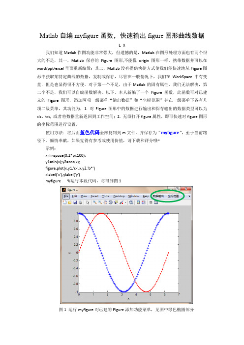
倾情奉献，如果觉得有参考或使用价值，请下载和评分哦~示例：x=linspace(0,2*pi,100);y1=sin(x);y2=cos(x);figure,plot(x,y1,'r.-',x,y2,'b*')xlabel('x'),ylabel('y')myfigure %运行本段代码，将得到图1图1 运行myfigure对已建的Figure添加功能菜单，见图中绿色椭圆部分1 坐标范围设置，如图2图2 通过单击“坐标范围”菜单下的坐标设置对坐标范围快速设置2 数据输出（至excel或txt或workspace）,如图3输出的数据格式，为若干列，一条曲线占两列，分别为x,y，多条则为x,y,x,y。

matlab中figure(1)的用法

在Matlab中，figure(1)是一个常用的指令，它用于创建一个新的图形窗口，并将其标记为1号窗口。

Figure(1)的用法非常灵活，可以用于绘制各种类型的图形，包括折线图、散点图、柱状图等。

在本文中，我们将讨论Figure(1)的基本用法，并结合实际代码和示例，帮助读者更深入地了解如何在Matlab中使用Figure(1)来创建和定制图形。

1. figure(1)的基本语法在Matlab中，可以通过简单的指令figure(1)来创建一个新的图形窗口，该指令的基本语法如下：```matlabfigure(1)```执行这条指令后，Matlab将会创建一个新的图形窗口，并将其标记为1号窗口，以便区分其他图形窗口。

接下来，我们将具体讨论如何在这个新建的图形窗口中绘制各种图形。

2. 绘制折线图Figure(1)可以用于绘制折线图，下面是一个简单的示例代码：```matlabx = 0:0.1:2*pi;y = sin(x);figure(1)plot(x, y)title('Sine Wave')xlabel('x')ylabel('sin(x)')```执行上述代码后，Figure(1)窗口将会显示一个标有“Sine Wave”的折线图，横轴为x，纵轴为sin(x)。

通过这个示例，读者可以了解如何在Figure(1)窗口中绘制简单的折线图，并添加标题、横纵坐标标签。

3. 绘制散点图除了折线图，Figure(1)还可以用于绘制散点图，下面是一个简单的示例代码：```matlabx = rand(1, 100);y = rand(1, 100);figure(1)scatter(x, y)title('Scatter Plot')xlabel('x')ylabel('y')```执行上述代码后，Figure(1)窗口将会显示一个标有“Scatter Plot”的散点图，横轴为x，纵轴为y。

matlab生成曲线

matlab生成曲线
MATLAB是一款功能强大的数学软件，在科学计算领域被广泛应用。

其中，生成曲线是MATLAB中常用的操作之一。

MATLAB提供了多种生成曲线的函数，主要有plot、scatter、line、surf等。

其中最常用的是plot函数。

使用plot函数可以生成不同类型的曲线，如折线图、散点图、
曲面图等。

其基本语法为：
plot(x,y)
scatter(x,y)
line(x,y)
其中，x和y分别是曲线的横坐标和纵坐标，可以是向量或矩阵。

对于折线图和曲面图，x和y需要是向量，而散点图可以使用矩阵表示。

除了基本的生成曲线函数，MATLAB还提供了丰富的功能，如添
加标题、轴标签、图例等。

这些功能可以通过设置图形属性来实现，如：
title('曲线图')
xlabel('横坐标')
ylabel('纵坐标')
legend('数据1','数据2')
通过以上设置，可以为生成的曲线添加标题、轴标签和图例，使其更加直观和易于理解。

总之，通过MATLAB生成曲线是一项常见的操作，使用plot等函数可以轻松实现，而丰富的功能设置则可以让生成的曲线更加精细和具有可读性。

matlab做曲线图参考资料(matlab做曲线图参考资料)

matlab做曲线图参考资料（matlab做曲线图参考资料）They can be used in combination. For example, "b-." stands for blue dot lines, "y:d" stands for yellow dashes, and marks data points with diamond characters. When the option is omitted, the MATLAB specifies that the lines are all solid lines, and the colors will follow the order of the curves.To set the curve style, you can add a drawing option to the plot function, with the call format as:Plot (x1, Y1, option 1, X2, Y2, option 2,... Xn, YN, option n)Example 1-6 in the same coordinate, the curves y1=0.2e-0.5xcos (4 PI x) and y2=2e-0.5xcos (PI x) are plotted with different linear shapes and colors respectively, and the intersection points of the two curves are marked.Procedures are as follows:X=linspace (0,2*pi, 1000);Y1=0.2*exp (-0.5*x).*cos (4*pi*x);Y2=2*exp (-0.5*x).*cos (pi*x);K=find (ABS (y1-y2) <1e-2);% lookup Y1 and Y2 equal (approximately equal) subscriptX1=x (k);% takes the X coordinate of Y1 and Y2Y3=0.2*exp (-0.5*x1).*cos (4*pi*x1);% Y1 y coordinates equalto Y2 valuesPlot (x, Y1, x, Y2,'k:', x1, Y3,'bp');1.4 graphics annotation and coordinate control1. graphic annotationThe format of the graph annotation function is called:Title (graphical name)Xlabel (x axis specification)Ylabel (Y axis specification)Text (x, y, graphical instructions)Legend (Legend 1, legend 2,... )The text in the function, in addition to using standard ASCII characters, you can also use LaTeX format control characters, so that you can add Greek letters, mathematical symbols and formulas on the graphics. For example, text (0.3,0.5, sin ({\omega}t+{\beta})) will get the annotation effect sin (omega t+ beta).In 0 cases of 1-7 = x = 2p interval and y2=cos curve y1=2e-0.5x (4 PI x), and to add graphics graphics mark.Procedures are as follows:X=0:pi/100:2*pi;Y1=2*exp (-0.5*x);Y2=cos (4*pi*x);Plot (x, Y1, x, Y2)Title ('x from 0 to 2{\pi}');% plus graphic titleXlabel ('Variable X');% plus X axis descriptionYlabel ('Variable Y');% plus Y axis descriptionText (0.8,1.5, 'curve y1=2e^{-0.5x}' ');% adds graphical descriptions at the specified locationText (2.5,1.1, 'curve y2=cos (4{\pi}x)');Legend (` Y1 ', ` Y2')% plus legend2. coordinate controlThe call format of the axis function is:Axis ([xmin, xmax, Ymin, ymax, Zmin, zmax])The axis function is rich in functionality, as well as in the usual formats:Axis equal: the vertical and horizontal axes are equal length scales.Axis Square: produces a square coordinate system (defaults to rectangles).Axis Auto: use default settings.Axis off: cancel the coordinate axis.Axis on: display axis.Give coordinates and mesh lines, and use the grid command to control. The grid on/off command controls whether to draw or not to draw the grid line, and the grid command without parameters switches between the two states.Add borders to the coordinates and use the box command to control them. The box on/off command controls whether to add or not to the border line, and the box command without arguments switches between the two states.Example 1-8 in the same coordinate, you can draw 3 concentric circles, plus coordinate control.Procedures are as follows:T=0:0.01:2*pi;X=exp (i*t);Y=[x; 2*x; 3*x]';Plot (y)Grid on;% plus mesh linesBox on;% plus coordinate bordersAxis equal% coordinate axes are used equal scale1.5 visual editing of graphicsThe MATLAB 6.5 version provides visual graphical editing tools in the graphical window, which can be used to edit various graphics objects in the window by using commands in the graphical window, menu bar, or toolbar.There is a menu bar and toolbar on the graphical window. The menu bar contains 7 menu items in File, Edit, View, Insert, Tools, Window, and Help. The toolbar contains 11 command buttons.1.6 drawing function of adaptive sampling of functionsThe call format of the fplot function is:Fplot (fname, LIMS, tol, options)Where fname is the function name, in the form of string, LIMS is x, y value range, tol is relative allowable error, and its system default value is 2e-3. The option definition is the sameas the plot function.Example 1-9 draws the curve of F (x) =cos (Tan (PI x)) with the fplot function.The commands are as follows:Fplot ('cos (Tan (pi*x)) ', [0,1], 1e-4]1.7 segmentation of graph windowThe call format of the subplot function is:Subplot (m, N, P)This function divides the current graphics window into m * n drawing areas, that is, each line is n, m lines in all, the area code is numbered by line, and the first p area is selected as the active area. In each drawing area, graphics are allowed to be drawn separately in different coordinate systems.Example 5-10 in the graphical window, a number of curves are plotted simultaneously in the form of subgraphs.Two. Other two-dimensional graphics2.1 2D data curves under other coordinate systems1. logarithmic coordinate graphicsMATLAB provides functions for plotting logarithmic and semilogarithmic coordinate curves:Semilogx (x1, Y1, option 1, X2, Y2, option 2,... )Semilogy (x1, Y1, option 1, X2, Y2, option 2,... )Loglog (x1, Y1, option 1, X2, Y2, option 2,... )2. polar diagramThe polar function is used to plot polar coordinates. The format of the call is:Polar (theta, rho, options)Where theta is the polar polar angle, Rho polar radius, content and function of similar options plot.Example 1-12 draws the polar diagram of r=sin (T) cos (T) and marks the data points.Procedures are as follows:T=0:pi/50:2*pi;R=sin (T).*cos (t);Polar (T, R,'-*');2.2 two-dimensional statistical analysis chartIn MATLAB, there are many two-dimensional statistical analysis graphs, such as bar graphs, ladder diagrams, bar graphs and filling graphs, etc. the functions used are:Bar (x, y, options)Stairs (x, y, options)Stem (x, y, options)Fill (x1, Y1, option 1, X2, Y2, option 2,... )Example 1-13 draw the curve y=2sin (x) with bar chart, ladder diagram, bar chart and filling chart respectively.Procedures are as follows:X=0:pi/10:2*pi;Y=2*sin (x);Subplot (2,2,1); bar (x, y,'g');Title ('bar (x, y,''g'')); axis ([0,7, -2,2]);Subplot (2,2,2); stairs (x, y,'b');Title ('stairs (x, y,''b'')); axis ([0,7, -2,2]);Subplot (2,2,3); stem (x, y,'k');Title ('stem (x, y,''k'')); axis ([0,7, -2,2]);Subplot (2,2,4); fill (x, y,'y');Title ('fill (x, y,''y'')); axis ([0,7, -2,2]);The statistical analysis functions provided by MATLAB are also many, such as pie charts, percentages of the elements that represent the sum of the elements, and so on.Example 1-14 drawing graphics:(1) the output value of an enterprise in each quarter (unit: 10000 yuan) is: 2347182720433025, the statistical analysis of the pie chart.(2) drawing the phasor graphs of complex numbers: 7+2.9i, 2-3i and -1.5-6i.Procedures are as follows:Subplot (1,2,1);Pie ([2347182720433025]);Title (pie chart);Legend ('Q1', 'two quarter', 'three quarter', 'fourth quarter');Subplot (1,2,2);Compass ([7+2.9i, 2-3i, -1.5-6i]);Title (` phasor diagram ');Three. Implicit function drawingMATLAB provides a ezplot function that draws implicit functions, and describes its usage.(1) for function f = f (x), the call of the ezplot function is in the form of:Ezplot (f): in the default interval, -2 PI <x<2 PI draws f = f (x) graphics.Ezplot (F, [a, b]): drawing f = f (x) in the interval a<x<b.(2) for implicit functions f = f (x, y), the call format of the ezplot function is:Ezplot (f): in the default interval, -2 PI <x<2 PI and -2 PI <y<2 PI draw graphs of F (x, y) = 0.Ezplot (F, [xmin),Xmax, Ymin, ymax]): draw graphs of F (x, y) = 0 in interval xmin<x<xmax and ymin<y<ymax.Ezplot (F, [a, b]): plots f (x, y) = 0 in interval a<x<b and a<y< B.(3) for parameter equations x = x (T) and y = y (T), the call format of the ezplot function is:Ezplot (x, y): in the default interval, 0<t<2 PI draws graphs of x=x (T) and y=y (t).Ezplot (x, y, [tmin, tmax]): in the interval Tmin < T < Tmax drawing x=x (T) and y=y (T) graphics.Example 1-15 implicit function drawing application example.Procedures are as follows:Subplot (2,2,1);Ezplot ('x^2+y^2-9'); axis equalSubplot (2,2,2);Ezplot ('x^3+y^3-5*x*y+1/5')Subplot (2,2,3);Ezplot ('cos (Tan (pi*x)) ', [0,1]]Subplot (2,2,4);Ezplot ('8*cos (T) ','4*sqrt (2) *sin (T)', [0,2*pi])Four. 3D graphics4.1 D curveThe plot3 function is very similar to the use of the plot function, and its call format is:Plot3 (x1, Y1, Z1, option 1, X2, Y2, Z2, option 2,... Xn, YN, Zn, option n)Each set of X, y, and Z forms the coordinates of a set of curves, and the definition of the option is the same as that of the plot function. When x, y, Z, vector, x, y, Z elements corresponding to a three-dimensional curve. When x, y, Z, matrix, with X, y, Z corresponding to the column element 3D curve, the curve is equal to the number of matrix columns.Example 1-16 draw three dimensional curve.Procedures are as follows:T=0:pi/100:20*pi;X=sin (t);Y=cos (t);Z=t.*sin (T).*cos (t);Plot3 (x, y, Z);Title ('Line, in, 3-D, Space');Xlabel ('X'); ylabel ('Y'); zlabel ('Z');Grid on;4.2 3D surface1. generate 3D dataIn MATLAB, meshgrid function is used to generate mesh coordinate matrix in plane region. Its format is:X=a:d1:b; y=c:d2:d;[X, Y]=meshgrid (x, y);When the statement is executed, each row of the matrix X is the vector x, the number of rows equal to the number of elements of the vector y, each column of the matrix Y is a vector y, and the number of columns is equal to the number of elements of the vector X.2. draw three-dimensional surface functionThe call format of the surf function and the mesh function is:Mesh (x, y, Z, c)Surf (x, y, Z, c)In general, x, y, and Z are matrices of the same dimension. X,y is the grid coordinate matrix, Z is the height matrix on the grid point, and C is used to specify the color range at different heights.Example 1-17 draw 3D surface graph z=sin (x+sin (y)) -x/10.Procedures are as follows:[x, y]=meshgrid (0:0.25:4*pi);Z=sin (x+sin (y)) -x/10;Mesh (x, y, Z);Axis ([0, 4*pi, 0, 4*pi, -2.5, 1]);In addition, there are 3D mesh surface functions meshc with contour lines and 3D mesh surface functions meshz with pedestal. Its usage is similar to that of mesh. The difference is that meshc draws the contours of the surface in the Z axis on the XY plane, and meshz draws the base of the surface on the XY plane.Example 1-18 in the XY plane, select the region [-8,8] * [-8,8], draw 4 kinds of three-dimensional surface map.Procedures are as follows:[x, y]=meshgrid (-8:0.5:8);Z=sin (sqrt (x.^2+y.^2))./sqrt (x.^2+y.^2+eps);Subplot (2,2,1);Mesh (x, y, Z);Title ('mesh (x, y, z) 'Subplot (2,2,2);Meshc (x, y, Z);Title ('meshc (x, y, z) 'Subplot (2,2,3);Meshz (x, y, z)Title ('meshz (x, y, z) 'Subplot (2,2,4);Surf (x, y, Z);Title ('surf (x, y, z) '3. standard 3D surfaceThe call format of the sphere function is: [x, y, z]=sphere (n)The call format of the cylinder function is:[x, y, z]=, cylinder (R, n)MATLAB also has a peaks function, called multimodal function, which is often used to demonstrate three-dimensional surfaces.<! --[if!Supportemptyparas] - > <! - [ENDIF] -- >例1 - 19 绘制标准三维曲面图形.程序如下:T = 0, PI / 20: 2 * PI;[x, y, Z] = cylinder (2) + sin (T), (30);Subplot (2,2,1);Surf (x, y, z);Subplot (2,2,2);[x, y, Z] = sphere;Surf (x, y, z);Subplot (2,1,2);[x, y, Z] = peaks (30);Surf (x, y, z);<! - [if. Supportemptyparas] - > <! - [ENDIF] -- >4.3 其他三维图形在介绍二维图形时, 曾提到条形图、杆图、饼图和填充图等特殊图形, 它们还可以以三维形式出现, 使用的函数分别是bar3、stem3、pie3 和fill3.Bar3函数绘制三维条形图, 常用格式为:Bar3 (y)Bar3 (x, y)Stem3函数绘制离散序列数据的三维杆图, 常用格式为:Stem3 (z)Stem3 (x, y, z)Pie3函数绘制三维饼图, 常用格式为:Pie3 (x)Fill3函数等效于三维函数fill, 可在三维空间内绘制出填充过的多边形, 常用格式为:Fill3 (x, y, Z, c)<! - [if. Supportemptyparas] - > <! - [ENDIF] -- > 例1 - 20 绘制三维图形:(1) 绘制魔方阵的三维条形图.(2) 以三维杆图形式绘制曲线y = 2Sin (x).(3) 已知x = [2347182720433025], 绘制饼图.(4) 用随机的顶点坐标值画出五个黄色三角形.程序如下:Subplot (2,2,1);Bar3 (Magic (4))Subplot (2,2,2);Y = 2 * sin (0, PI / 10: 2 * PI);Stem3 (y);Subplot (2,2,3);Pie3 ([2347182720433025]);Subplot (2,2,4);Fill3 (rand (3,5), Rand (3,5), Rand (3,5), 'y')例1 - 21 绘制多峰函数的瀑布图和等高线图.程序如下:Subplot (1,2,1);[x, y, Z] = peaks (30);Waterfall (x, y, z)Xlabel (x axis), ylabel (Y - axis), zlabel (Z - axis). Subplot (1,2,2);Contour3 (x, y, Z, 12, 'k');% 其中12代表高度的等级数Xlabel (x axis), ylabel (Y - axis), zlabel (Z - axis). <! - [if. Supportemptyparas] -- >图形修饰处理五.5.1 视点处理Matlab提供了设置视点的函数view, 其调用格式为:The view (AZ, EL)其中az为方位角, el为仰角, 它们均以度为单位.系统缺省的视点定义为方位角 - 37.5°, 仰角30°.例5 - 22 从不同视点观察三维曲线.5.2 色彩处理1.颜色的向量表示Matlab除用字符表示颜色外, 还可以用含有3个元素的向量表示颜色.向量元素在 [0,1] 范围取值, 3个元素分别表示红、绿、蓝3种颜色的相对亮度, 称为rgb三元组.<! - [if. Supportemptyparas] - > <! - [ENDIF] -- >2.色图色图 (color map) 是matlab系统引入的概念.在matlab中, 每个图形窗口只能有一个色图.色图是m×3 的数值矩阵, 它的每一行是rgb三元组.色图矩阵可以人为地生成, 也可以调用matlab提供的函数来定义色图矩阵.3.三维表面图形的着色三维表面图实际上就是在网格图的每一个网格片上涂上颜色.surf函数用缺省的着色方式对网格片着色.除此之外, 还可以用shading命令来改变着色方式.Shading faceted命令将每个网格片用其高度对应的颜色进行着色, 但网格线仍保留着, 其颜色是黑色.这是系统的缺省着色方式.Shading flat命令将每个网格片用同一个颜色进行着色, 且网格线也用相应的颜色,This makes the surface of the graphics more smooth.The shading interp command uses color interpolation in mesh slices to get the most smooth surface.1-233 examples of graphic shading effects are presented.Procedures are as follows:[x, y, z]=sphere (20);Colormap (copper);Subplot (1,3,1);Surf (x, y, Z);Axis equalSubplot (1,3,2);Surf (x, y, z); shading flat;Axis equalSubplot (1,3,3);Surf (x, y, z); shading interp;Axis equal5.3 light treatmentMATLAB provides the function of lighting settings, which is called:Light ('Color', option 1,'Style', option 2,'Position', option 3)< --[if! SupportEmptyParas]--> <! --[endif]-->!Example 5-24 spherical surface after illumination.Procedures are as follows:[x, y, z]=sphere (20);Subplot (1,2,1);Surf (x, y, z); axis equal;Light ('Posi', [0,1,1]);Shading interp;Hold on;Plot3 (0,1,1,'p'); text (0,1,1,' light'');Subplot (1,2,2);Surf (x, y, z); axis equal;Light ('Posi', [1,0,1]);Shading interp;Hold on;Plot3 (1,0,1,'p'); text (1,0,1,' light'');5.4 graphics cutting processingExample 5-25 draw three-dimensional surface map, and interpolation coloring processing, cut off the graph, X and y are less than 0 parts.Procedures are as follows:[x, y]=meshgrid (-5:0.1:5);Z=cos (x),.*cos (y),.*exp (-sqrt (x.^2+y.^2), /4);Surf (x, y, z); shading interp;Pause% program pauseI=find (x<=0&y<=0);Z1=z; Z1 (I) =NaN;Surf (x, y, z1); shading interp;To show the clipping effect, the first surface is paused after the drawing is finished, and then the trimmed surface is displayed.Six. Image processing and animation making6.1 image processing1.imread and imwrite functionsThe imread and imwrite functions are used to read the image file into the MATLAB workspace, and to combine the image data with the color chart data into a certain format of the image file. MATLAB supports a variety of image file formats, suchas.Bmp,.Jpg,.Jpeg,.Tif and so on.2.image and imagesc functionsThese two functions are used for image display. In order to ensure the image display effect, the general colormap function should also be used to set the image color chart.Example 1-26 has an image file, flower.jpg, which displays the image in the graphical window.Procedures are as follows:[x, cmap]=imread ('flower.jpg');% read data array and color maparray of imageImage (x); colormap (CMAP);Axis, image, off%, keep the aspect ratio, and cancel the axis6.2 animationMATLAB provides getframe, moviein, and movie functions for animation.1.getframe functionThe getframe function intercepts a picture information (called a frame in an animation), and a picture information forms a very large column vector. Obviously, you need a large matrix to save the N map surface.2.moviein functionThe moviein (n) function is used to create a large enough n column matrix. The matrix is used to hold data from N frames for playback. The reason why we have to build a large matrix in advance is to improve the speed of the program.3.movie functionThe movie (m, n) function plays the screen defined by the matrix n times m, and is played by default.Example 1-27 draws the peaks function surface and rotates itaround the Z axis.Procedures are as follows[X, Y, Z]=peaks (30);Surf (X, Y, Z)Axis ([-3,3, -3,3, -10,10])Axis off;Shading interp;Colormap (hot);M=moviein (20);% establishes a large 20 column matrix For i=1:20View (-37.5+24* (i-1), 30)% change view pointM (:: I) =getframe;% saves graphics to the M matrix EndMovie (m, 2);% play screen 2 times。

输出Matlab画的图的一个方法

输出Matlab画的图的一个方法输出Matlab 画的图的一个方法已有215 次阅读2012-5-7 08:58|系统分类:科研笔记|关键词:matlab 输出图形 figure exportfig经常看到有些人用 Matlab 画图后保存为 EPS 格式或者 PNG 格式的图时字体太小。

不太美观。

这里把我常用的比较好方法和大家分享一下，也给自己和学生留个印记。

附件的exportfig.m 程序可以很好地把Matlab 画的图输出为很多格式的文件，并且可以设置字体的大小，颜色等，使用方便灵活。

用法很简单，把这个文件放在Matlab 的搜索目录中（最简单就是当前的工作目录）。

然后：fig=figure(1); % 定义一个 fig 的图形句柄.... % 这里用 plot 等函数画图..exportfig(fig, 'fig2.eps', 'FontMode', 'fixed','FontSize', 10, 'color', 'cmyk' ); % 把上面画的图（句柄为 fig ）保存为 fig2.eps, 字号为 10，彩色。

运行以后就可以在当前目录看到一个名为 fig2.eps 的文件了。

这个 exportfig() 函数含有很多选项可以灵活设置，详看下面的说明：%EXPORTFIG Export a figure to Encapsulated Postscript.% EXPORTFIG(H, FILENAME) writes the figure H to FILENAME.H is% a figure handle and FILENAME is a string that specifies the % name of the output file.%% EXPORTFIG(...,PARAM1,VAL1,PARAM2,VAL2,...) specifies% parameters that control various characteristics of the output% file.%% Format Paramter:% 'Format' one of the strings 'eps','eps2','jpeg','png','preview' % specifies the output format. Defaults to 'eps'.% The output format 'preview' does not generate an output % file but instead creates a new figure window with a% preview of the exported figure. In this case the% FILENAME parameter is ignored.%% 'Preview' one of the strings 'none', 'tiff'% specifies a preview for EPS files. Defaults to 'none'.%% Size Parameters:% 'Width' a positive scalar% specifies the width in the figure's PaperUnits% 'Height' a positive scalar% specifies the height in the figure's PaperUnits%% Specifying only one dimension sets the other dimension % so that the exported aspect ratio is the same as the% figure's current aspect ratio.% If neither dimension is specified the size defaults to% the width and height from the figure's PaperPosition.%% Rendering Parameters:% 'Color' one of the strings 'bw', 'gray', 'cmyk'% 'bw' specifies that lines and text are exported in% black and all other objects in grayscale% 'gray' specifies that all objects are exported in grayscale % 'cmyk' specifies that all objects are exported in color% using the CMYK color space% 'Renderer' one of the strings 'painters', 'zbuffer', 'opengl' % specifies the renderer to use% 'Resolution' a positive scalar% specifies the resolution in dots-per-inch.%% The default color setting is 'bw'.%% Font Parameters:% 'FontMode' one of the strings 'scaled', 'fixed'% 'FontSize' a positive scalar% in 'scaled' mode multiplies with the font size of each% text object to obtain the exported font size% in 'fixed' mode specifies the font size of all text% objects in points% 'FontEncoding' one of the strings 'latin1', 'adobe'% specifies the character encoding of the font%% If FontMode is 'scaled' but FontSize is not specified then a % scaling factor is computed from the ratio of the size of the % exported figure to the size of the actual figure. The minimum% font size allowed after scaling is 5 points.% If FontMode is 'fixed' but FontSize is not specified thenthe % exported font sizes of all text objects is 7 points.%% The default 'FontMode' setting is 'scaled'.%% Line Width Parameters:% 'LineMode' one of the strings 'scaled', 'fixed'% 'LineWidth' a positive scalar% the semantics of LineMode and LineWidth are exactly the % same as FontMode and FontSize, except that they apply % to line widths instead of font sizes. The minumum line% width allowed after scaling is 0.5 points.% If LineMode is 'fixed' but LineWidth is not specified% then the exported line width of all line objects is 1% point.%% Examples:% exportfig(gcf,'fig1.eps','height',3);% Exports the current figure to the file named 'fig1.eps' with % a height of 3 inches (assuming the figure's PaperUnits is % inches) and an aspect ratio the same as the figure's aspect % ratio on screen.%% exportfig(gcf, 'fig2.eps', 'FontMode', 'fixed',...% 'FontSize', 10, 'color', 'cmyk' );% Exports the current figure to 'fig2.eps' in color with all % text in 10 point fonts. The size of the exported figure is % the figure's PaperPostion width and height.。

matlab图像输出设置

matlab图像输出设置核⼼⽅法：通过图像设置命令，直接指定图⽚的⼤⼩。

具体操作：(1) 完成画图及相关设置(字体⼤⼩、线宽、图例⼤⼩也是正常尺⼨)，(2) 此时WindowStyle is 'docked'，要改为normal，有两种操作：1)在Figure properties——more properties中找到Windowstyle，然后⽤⿏标改为normal；2)或者直接⽤命令：set (gcf,'windowstyle','normal')(3) 根据排版要求，确定图⽚的宽⾼，例如320*320 像素，然后使⽤命令set (gcf,'Position',[500,300,320,320])set(gcf,'Units','centimeters','Position',[100 100 9 8]);% figure的position中的[left bottom width height] 是指figure的可画图的部分的左下⾓的坐标以及宽度和⾼度。

(4) 使⽤copy figure将图⽚输出到Word1.figure;2.hold on;3.set(gca, 'YTick', [0 : 0.2 : 1]);4.box off;5.set(gca, 'YTickLabel', {'matlab1', 'matlab2', 'matlab3',...6. 'matlab4', 'matlab5', 'matlab6'})1.hold on2.xL=xlim;3.yL=ylim;4.plot(xL,[yL(2),yL(2)],'k',[xL(2),xL(2)],[yL(1),yL(2)],'k')5.box off6.axis([xL yL])1.t=linspace(0,8,100);%%% linspace(X1, X2) generates a row vector of 100 linearlyequally spaced points between X1 and X2.linspace(X1, X2, N) generates N points between X1 and X2.2.a1=axes;%% axes Create axes in arbitrary positions.axes('position', RECT) opens up an axis at the specifiedlocation and returns a handle to it.RECT = [left, bottom, width, height] specifies the location and size of the side of the axis box, relative to the lower-left corner of the Figure window, in normalized units where (0,0) is the lower-left corner and (1.0,1.0) is the upper-right.3.plot(t,sin(t));4.xt=get(gca,'xtick');5.set(gca,'XTick',[],'XColor','w');6.xL=xlim;7.p=get(gca,'Position');8.box off;1.figure2.a2=axes('Position',p+[0,p(4)/2,0,-p(4)/2]); % 确定坐标位置，p为上述3.xlim(xL); %定义x轴坐标4.box off;5.set(gca,'XTick',xt,'Color','None','YTick',[]);简单点⼉说吧：xtick是刻度（⼩竖线）；xticklabel 刻度值（竖线下⾯的数值）。

figure函数

figure函数
Figure函数用来在Python中创建图形。

它是matplotlib库的一部分，能够帮助你将数据可视化，以便更好地理解和分析数据。

figure函数能够创建并管理图形，并包含多个子图形。

这些子图形可以包含不同的图表类型，例如折线图、散点图、柱状图等。

要使用figure函数，首先需要导入matplotlib库。

然后，你可以使用figure函数来创建一个新的图形，并指定图形的大小和分辨率。

例如，使用以下代码可以创建一个8英寸x6英寸的图形，分辨率为200 dpi：
fig = plt.figure(figsize=(8,6), dpi=200)
接下来，你可以使用add_subplot函数在图形中添加子图形。

例如，要添加一个折线图，可以使用以下代码：
ax = fig.add_subplot(1,1,1)
ax.plot(x,y)
这里，ax是子图形的句柄，从而可以使用其他matplotlib函数来格式化子图形，例如设置图例、坐标轴标签等。

最后，当你完成绘图时，可以使用show函数显示图形。

通过使用figure函数，你可以更轻松地创建图形，并自定义大小和
分辨率。

它可以帮助你以可视化的方式分析数据，从而使你的分析更有效率。

因此，使用figure函数可以极大地提高你的分析效率。

Matlab自编myfigure函数,快速输出figure图形曲线数据(原创)

对于第一个不足，由于Matlab的固有属性，我们无法解决，第二个不足，我们可以自编函数解决。

使用方法：将后面蓝色代码全部复制到m文件，并保存为“myfigure”，至于当前路径下。

如何用Matlab绘制曲线图

如何用Matlab绘制曲线图各位同学：在写论文和报告时，为了很好地表达你研究和开发的结果，不仅要用文字详细地描述你方法、步骤和结果，还必须配以各种图来说明问题。

下面是我们实验室张媛媛老师申请博士学位论文中的部分曲线图、硬件框图、软件流程图和实验装置原理框图。

她将在部分曲线图下面给出绘制图形的Matlab 程序和相关步骤，供大家学习和参考。

例一：-0.500.511.522.5Time(s)V o l t a g e (V )12-0.50.511.522.5时间(s)电压(V )12图2-3-6 动态线性环节的输入输出信号图2-3-7 模型输出和消噪后实验时数据比较1,输入信号u(k)；2,输出信号y(k) 1,实验数据；2,模型输出绘图程序如下： figure(1)plot(t,y,'k',t,x,'k','LineWidth',1.4)xlabel('Time(s)','fontname','宋体','Fontsize',9);％绘制横坐标 ylabel('Voltage(v)','fontname','宋体','Fontsize',9); ％绘制纵坐标%xlabel('时间(s)','fontname','宋体','Fontsize',9);%ylabel('电压(v)','fontname','宋体','Fontsize',9);％设置合适的图框大小.可将下面四句变为子程序，以便调用。

set(gcf,'color',[1,1,1]);set(gca,'xcolor',[0,0,0],'ycolor',[0,0,0]);set(gcf,'units','centimeters','position',[5,10,6.8,5.2]);set(gca,'box','on','fontname','宋体','Fontsize',9);％设置指向线的位置annotation1 = annotation(figure(1),'line',[0.5585 0.6038],[0.7225 0.6459]); annotation1 = annotation(figure(1),'line',[0.4755 0.4453],[0.7129 0.6651]); ％标注数字“1”“2”annotation1 = annotation(...figure(1),'textbox',...'Position',[0.3849 0.5486 0.3396 0.1404],...'LineStyle','none',...'FontSize',8,...'String',{'1'},...'FitHeightToText','on');annotation1 = annotation(...figure(1),'textbox',...'Position',[0.5974 0.5382 0.3396 0.1404],...'LineStyle','none',...'FontSize',8,...'String',{'2'},...'FitHeightToText','on');例二：020*********电压(v)质量流量(g /s )1,实验数据2,拟合曲线12图2-4-3 '(.)f 的静态特性绘图程序如下： figure(1)plot(t,y,'k',t,x,'k','LineWidth',1.4)xlabel('时间(s)','fontname','宋体','Fontsize',9); ylabel('质量流量(g/s)','fontname','宋体','Fontsize',9); legend('1,实验数据','2,拟合曲线')※ ※当根据程序画出的线段位置不理想时，可用下面的步骤来做。

巧用matlab提取图片中的曲线数据(修订版)

利用Matlab提取图片中的数据(修订版)从事科研或者工程的人员在文档撰写过程中，常需要将文献中的曲线与自己的结果对比，为获取原始数据，一种常用的办法是手动描点，即将原始曲线放大然后打印出来，选取一定数量的点，读出其横纵坐标，然后重绘。

对于较为平坦的曲线，这种方法当然可行，但当曲线数量增加，曲线变化复杂，这种方法工作量可想而知。

前段时间由于原始数据丢失，仅剩几十幅图片，本人尝试过手动描点，经历几个小时奋战，实在无法继续，索性转向matlab，借助其强大的数据处理能力，编写了两个GUI的小软件image2data、data_poly提取数据，如今大功告成，遂于大家分享。

2010-12-26yc97463240@2010年编写软件至今，已有一年，平均每个星期都有网友向我索要软件或提出问题，与你们的交流很愉快，为答谢大家对我的鼓励，我决定：1、对本教程作出修改，针对大家容易出现错误的地方作出批注，并在一个月内对程序进行改进。

2、录制视频教程，更加直接的引导大家使用。

最后申明，本教程完全免费，可在百度、豆丁和其他文档分享类网站在线阅览，教程会发布到优酷上，如有需要，直接email索取(一般当天回复)。

2012-03-10yc97463240@本文分三部分：1、数据提取实验演示；2、软件编写要点；3、附录。

关心使用操作的朋友请看第一部分，有兴趣钻研代码的朋友请看第二部分，本软件以功能实现为主，界面和操作方面略有不适，尽请谅解。

1、数据提取演示实验原始数据来源：安华高科技数据手册（HSMP-38XX and HSMP-48XX Series），如图1所示。

目标曲线：提取1MHz频率下的PIN二极管电容与反偏电压之间关系曲线。

图1 包含目标曲线的原始图像实验步骤：Step1：制作jpg图片方法：利用PPT的图片另存功能制作jpg图片，本方法具有普遍性。

首先从pdf中copy图1，即上述包含数据坐标的曲线，然后paste到ppt的空白页面，最后调整图片大小，另存为 figure1.jpg，如图2所示。

matlab figure的用法

文章标题：探索MATLAB Figure的用法1. 引言MATLAB作为一种常用的科学计算软件，其图形绘制功能十分强大。

其中，Figure作为MATLAB中的绘图窗口，提供了丰富的功能和灵活的操作方式，能够帮助用户实现各种复杂的图形展示和数据可视化。

在本文中，将深入探讨MATLAB Figure的用法，帮助读者更好地理解和应用这一功能。

2. MATLAB Figure的基本操作在MATLAB中，Figure是用来显示图形的窗口。

通过简单的命令，可以创建、操作和定制Figure窗口。

在创建Figure时，可以指定标题、大小、位置等属性，以及添加各种绘图元素，如曲线、散点图、柱状图等。

通过设定坐标轴范围、刻度、标签等属性，可以使图形更加清晰、直观。

还可以通过设置图例、注释和标题等元素，使图形更具可读性和美观性。

3. MATLAB Figure的高级功能除了基本的图形绘制功能外，MATLAB Figure还提供了丰富的高级功能，如图形交互、三维绘图、动态图形、多图合并等。

通过设置交互式图形，可以让用户与图形进行交互，实现数据筛选、放大缩小、数据标注等操作。

在三维绘图方面，MATLAB Figure可以实现3D曲面、立体图、体绘图等，展示更加复杂和丰富的数据结构。

也可以利用动态图形功能，实现对数据的实时展示和动态变化的可视化。

通过多图合并，可以将多个图形组合在一个Figure窗口中，进行比较和分析。

4. 个人观点和理解在我看来，MATLAB Figure的用法不仅仅限于简单的图形展示，更重要的是其在科学计算和数据分析中的应用。

通过合理地利用MATLAB Figure的功能，可以实现对复杂数据的可视化和分析，进而发现数据中的规律和特点。

也可以借助MATLAB Figure，与其他功能模块结合，实现对数据的处理和解读。

对MATLAB Figure的深入了解与熟练运用，可以帮助我们更好地进行科学研究和工程应用。

MATLAB输出图像

这两天碰到一个问题是关于用 MATLAB 命令把示波器图形画出，经过努力总算得到解决。
看到网上有的同行问怎么改示波器的背景，把示波器波形复制到 Word 中，我有两种方法，第一种是我一个同学告诉我的，通过命令对示波器进行操作。具体如下 shh = get(0,'ShowHiddenHandles'); set(0,'ShowHiddenHandles','On'); set(gcf,'menubar','figure'); set(gcf,'CloseRequestFcn','closereq'); set(gcf,'DefaultLineClipping','Off'); set(0,'ShowHiddenHandles',shh) 输入以上命令可以直接对示波器进行修改，包括背景和曲线颜色第二种方法我以前总结过，现在详细说明一下用 MATLAB 命令将 simulink 示波器的图形画出第一步，将你的示波器的输出曲线以矩阵形式映射到 MATLAB 的工作空间内。如图1所示，双击示波器后选择 parameters 目录下的 Data history,将 Save data to workspace 勾上，Format 选择 Array,Variable name 即你输入至工作空间的矩阵名称，这里我取名 aa。在这之后运行一次仿真，那么你就可以在 MATLAB 的工作空间里看到你示波器输出曲线的矩阵 aa。如图2所示。
理解曲线矩阵的原理之后，我们就可以用 plot 函数画出示波器中显示的图形了。 curve=plot(aa(:,1),aa(:,2),aa(:,1),aa(:,3),'--r') � (:,1)表示取 aa 的第一列，仿真时间 � (:,2)表示取 aa 的第二列，示波器的输入一 � (:,3)表示取 aa 的第三列，示波器的输入二 %--r 表示曲线2显示的形式和颜色，这里是（red) set(curve(1),'linewidth',3) %设置曲线1的粗细 set(curve(2),'linewidth',3) %设置曲线2的粗细 legend('Fuzzy','PID') %曲线名称标注 xlabel('仿真时间（s）') %X 坐标轴名称标注 ylabel('幅值') %Y 轴坐标轴标注 title('Fuzzy Control VS PID') %所画图的名称 grid on

利用Matlab提取图片中曲线数据(线性修正,支持对数坐标)

利用Matlab提取图片中曲线数据前一段时间看到一篇文章“利用Matlab提取图图片中的数据”，觉得思路挺好，遂下载下来研究了一番，发现作者所编写的程序没有考虑原始图片非水平放置的情况，而实际扫描图片时，将图片完全放置水平难度较大... 同时作者也没有考虑对数坐标的情况，且程序GUI界面不太人性化，操作有点不习惯。

因此借着作者良好意愿，对其程序进行了改进~2011-6-9shanyunh@ 考虑一张非水平无变形的曲线图，现将其曲线数据取出来，步骤如下：(x(x11.在坐标轴上取三点以定位坐标系。

如图中红色点所示。

2.在曲线上选取若干个点，如图中蓝色点所示。

3.设定坐标轴选取点x和y的实际值。

4.选取坐标系类型。

5.变换。

6.保存数据。

7.数据后处理。

在变换过程中程序首先计算(xi,yi)到(x1,y1)和(x2,y2)所组成的y轴的距离Δx，同样的方法计算Δy，当然Δx和Δy是图片的像素值。

接下来计算每个像素点所对应实际坐标值。

对于线性x轴，比例系数为(Xmax-Xmin)/(sqrt((x1-x0)^2)+(y1-y0)^2)，同样对于线性y轴，比例系数(Ymax-Ymin)/(sqrt((x0-x2)^2)+(y0-y2)^2)。

这样即可求出每个点的实际坐标值Xi=Δx *(Xmax-Xmin)/(sqrt((x1-x0)^2)+(y1-y0)^2)+XminYi=Δy *(Ymax-Ymin)/(sqrt((x0-x2)^2)+(y0-y2)^2)+Ymin对数坐标的变换关系类似Xi=10^(log10(Xmin)+Δx *(log10(Xmax)-log10(Xmin))/(sqrt((x1-x0)^2)+(y1-y0)^2))Yi= 10^(log10(Ymin)+Δy *(log10(Ymax)-log10(Ymin))/(sqrt((x0-x2)^2)+(y0-y2)^2))具体操作说明1.导入图片。

matlab导出曲线数据的函数

在MATLAB中，导出曲线数据是一个常见的需求。

通常，我们需要将所得到的曲线数据保存到外部文件中，以便进行进一步的分析和处理。

在MATLAB中，有多种方法可以实现曲线数据的导出，包括使用内置函数、自定义函数以及第三方工具包等。

在本文中，我们将就MATLAB中导出曲线数据的函数进行全面评估，并探讨不同方法的优缺点，以及个人观点和理解。

1. 使用内置函数MATLAB提供了许多内置函数，可以帮助我们轻松地导出曲线数据。

其中最常用的函数是`dlmwrite`和`writematrix`。

这两个函数都可以将数值矩阵写入到文本文件中，非常方便且简单。

我们可以使用如下代码将曲线数据保存到一个名为`data.txt`的文本文件中：```matlabx = 1:10;y = sin(x);data = [x' y'];dlmwrite('data.txt', data, 'delimiter', '\t');```使用内置函数的优点是操作简单，代码量少，适用于快速导出小规模的曲线数据。

然而，这种方法也存在一些局限性，例如无法自定义输出格式、无法导出带有文本信息的数据等。

2. 自定义函数除了使用内置函数外，我们还可以编写自定义函数来实现曲线数据的导出。

通过编写自定义函数，我们可以更加灵活地控制导出的格式、内容以及文件命名等方面。

我们可以编写一个名为`exportData`的函数来实现曲线数据的导出：```matlabfunction exportData(filename, x, y)fid = fopen(filename, 'w');fprintf(fid, 'x\ty\n');for i=1:length(x)fprintf(fid, '%f\t%f\n', x(i), y(i));endfclose(fid);end```使用自定义函数的优点是可以完全按照需求进行定制，可以处理更加复杂的数据导出任务。

figure的matlab原理与功能

"figure"是MATLAB中用来创建和管理图形窗口的重要函数。

在本文中，我们将深入探讨figure的原理和功能，从简单到复杂地解释其背后的原理，并探讨如何利用figure函数创建各种类型的图形。

1. figure函数的基本原理figure函数在MATLAB中的基本原理是创建一个新的图形窗口，并将焦点切换到该窗口上。

这意味着在同一时间内可以同时显示多个图形，而不会相互覆盖。

figure函数还可以通过设置不同的属性值，如窗口大小、标题、背景色等，以及调整显示位置等，来实现对图形窗口的灵活管理。

2. figure函数的基本功能figure函数不仅可以用来创建新的图形窗口，还可以在一个图形窗口中显示多个子图形。

通过子图形的分割和管理，可以实现复杂图形的同时展示，并轻松将不同的图形进行比较和分析。

在图形窗口中，还可以通过鼠标交互式地调整图形的显示和参数，以更好地呈现数据的特征和规律。

3. figure函数的高级功能除了上述基本功能外，figure函数还提供了许多高级功能，如创建3D 图形、动态更新图形、图形叠加、保存和导出图形等。

通过这些高级功能，可以实现更加复杂和丰富的数据可视化和分析，为科学研究和工程应用提供了强大的支持。

总结回顾：通过本文的深入探讨，我们对figure函数的原理和功能有了更加深入的了解。

了解了它的基本原理和功能之后，我们还探讨了其高级功能，并且对如何利用figure函数进行数据可视化和分析有了更清晰的认识。

figure函数作为MATLAB的重要组成部分，为我们进行科学研究和工程实践提供了方便和高效的图形展示和分析工具。

个人观点和理解：在我的实际工作中，我经常使用figure函数来展示和分析实验数据，通过合理设置图形窗口的样式和参数，以及灵活使用子图形功能，可以更清晰地呈现数据的特征和规律。

figure函数的高级功能也为我提供了丰富的操作和展示效果，使得我的工作能够更加高效和专业。