A Fast Algorithm for Statistically Optimized Orientation Estimation
FastICA 1.2-4 快速独立成分分析算法说明书

Package‘fastICA’November27,2023Version1.2-4Date2023-11-27Title FastICA Algorithms to Perform ICA and Projection PursuitAuthor J L Marchini,C Heaton and B D Ripley<***************>Maintainer Brian Ripley<***************>Depends R(>=4.0.0)Suggests MASSDescription Implementation of FastICA algorithm to perform IndependentComponent Analysis(ICA)and Projection Pursuit.License GPL-2|GPL-3NeedsCompilation yesRepository CRANDate/Publication2023-11-2708:34:50UTCR topics documented:fastICA (1)ica.R.def (5)ica.R.par (6)Index7 fastICA FastICA algorithmDescriptionThis is an R and C code implementation of the FastICA algorithm of Aapo Hyvarinen et al.(https: //www.cs.helsinki.fi/u/ahyvarin/)to perform Independent Component Analysis(ICA)and Projection Pursuit.1UsagefastICA(X,p,alg.typ=c("parallel","deflation"),fun=c("logcosh","exp"),alpha=1.0,method=c("R","C"),row.norm=FALSE,maxit=200,tol=1e-04,verbose=FALSE,w.init=NULL)ArgumentsX a data matrix with n rows representing observations and p columns representing variables.p number of components to be extractedalg.typ if alg.typ=="parallel"the components are extracted simultaneously(the default).if alg.typ=="deflation"the components are extracted one at atime.fun the functional form of the G function used in the approximation to neg-entropy (see‘details’).alpha constant in range[1,2]used in approximation to neg-entropy when fun== "logcosh"method if method=="R"then computations are done exclusively in R(default).The code allows the interested R user to see exactly what the algorithm does.ifmethod=="C"then C code is used to perform most of the computations,whichmakes the algorithm run faster.During compilation the C code is linked to anoptimized BLAS library if present,otherwise stand-alone BLAS routines arecompiled.row.norm a logical value indicating whether rows of the data matrix X should be standard-ized beforehand.maxit maximum number of iterations to perform.tol a positive scalar giving the tolerance at which the un-mixing matrix is considered to have converged.verbose a logical value indicating the level of output as the algorithm runs.w.init Initial un-mixing matrix of dimension c(p,p).If NULL(default) then a matrix of normal r.v.’s is used.DetailsIndependent Component Analysis(ICA)The data matrix X is considered to be a linear combination of non-Gaussian(independent)compo-nents i.e.X=SA where columns of S contain the independent components and A is a linear mixing matrix.In short ICA attempts to‘un-mix’the data by estimating an un-mixing matrix W where XW =S.Under this generative model the measured‘signals’in X will tend to be‘more Gaussian’than the source components(in S)due to the Central Limit Theorem.Thus,in order to extract the independent components/sources we search for an un-mixing matrix W that maximizes the non-gaussianity of the sources.In FastICA,non-gaussianity is measured using approximations to neg-entropy(J)which are more robust than kurtosis-based measures and fast to compute.The approximation takes the formJ(y)=[E{G(y)}−E{G(v)}]2where v is a N(0,1)r.v.log cosh(αu)and G(u)=−exp(u2/2).The following choices of G are included as options G(u)=1αAlgorithmFirst,the data are centered by subtracting the mean of each column of the data matrix X.The data matrix is then‘whitened’by projecting the data onto its principal component directionsi.e.X->XK where K is a pre-whitening matrix.The number of components can be specified bythe user.The ICA algorithm then estimates a matrix W s.t XKW=S.W is chosen to maximize the neg-entropy approximation under the constraints that W is an orthonormal matrix.This constraint en-sures that the estimated components are uncorrelated.The algorithm is based on afixed-point iteration scheme for maximizing the neg-entropy.Projection PursuitIn the absence of a generative model for the data the algorithm can be used tofind the projection pursuit directions.Projection pursuit is a technique forfinding‘interesting’directions in multi-dimensional datasets.These projections and are useful for visualizing the dataset and in density estimation and regression.Interesting directions are those which show the least Gaussian distribu-tion,which is what the FastICA algorithm does.ValueA list containing the following componentsX pre-processed data matrixK pre-whitening matrix that projects data onto thefirst p principal compo-nents.W estimated un-mixing matrix(see definition in details)A estimated mixing matrixS estimated source matrixAuthor(s)J L Marchini and C HeatonReferencesA.Hyvarinen and E.Oja(2000)Independent Component Analysis:Algorithms and Applications,Neural Networks,13(4-5):411-430See Alsoica.R.def,ica.R.parExamples#---------------------------------------------------#Example1:un-mixing two mixed independent uniforms#---------------------------------------------------S<-matrix(runif(10000),5000,2)A<-matrix(c(1,1,-1,3),2,2,byrow=TRUE)X<-S%*%Aa<-fastICA(X,2,alg.typ="parallel",fun="logcosh",alpha=1,method="C",row.norm=FALSE,maxit=200,tol=0.0001,verbose=TRUE)par(mfrow=c(1,3))plot(a$X,main="Pre-processed data")plot(a$X%*%a$K,main="PCA components")plot(a$S,main="ICA components")#--------------------------------------------#Example2:un-mixing two independent signals#--------------------------------------------S<-cbind(sin((1:1000)/20),rep((((1:200)-100)/100),5))A<-matrix(c(0.291,0.6557,-0.5439,0.5572),2,2)X<-S%*%Aa<-fastICA(X,2,alg.typ="parallel",fun="logcosh",alpha=1,method="R",row.norm=FALSE,maxit=200,tol=0.0001,verbose=TRUE)par(mfcol=c(2,3))plot(1:1000,S[,1],type="l",main="Original Signals",xlab="",ylab="")plot(1:1000,S[,2],type="l",xlab="",ylab="")plot(1:1000,X[,1],type="l",main="Mixed Signals",xlab="",ylab="")plot(1:1000,X[,2],type="l",xlab="",ylab="")plot(1:1000,a$S[,1],type="l",main="ICA source estimates",xlab="",ylab="")plot(1:1000,a$S[,2],type="l",xlab="",ylab="")#-----------------------------------------------------------#Example3:using FastICA to perform projection pursuit on a#mixture of bivariate normal distributions#-----------------------------------------------------------if(require(MASS)){x<-mvrnorm(n=1000,mu=c(0,0),Sigma=matrix(c(10,3,3,1),2,2)) x1<-mvrnorm(n=1000,mu=c(-1,2),Sigma=matrix(c(10,3,3,1),2,2)) X<-rbind(x,x1)a<-fastICA(X,2,alg.typ="deflation",fun="logcosh",alpha=1,ica.R.def5 method="R",row.norm=FALSE,maxit=200,tol=0.0001,verbose=TRUE)par(mfrow=c(1,3))plot(a$X,main="Pre-processed data")plot(a$X%*%a$K,main="PCA components")plot(a$S,main="ICA components")}ica.R.def R code for FastICA using a deflation schemeDescriptionR code for FastICA using a deflation scheme in which the components are estimated one by one.This function is called by the fastICA function.Usageica.R.def(X,p,tol,fun,alpha,maxit,verbose,w.init)ArgumentsX data matrixp number of components to be extractedtol a positive scalar giving the tolerance at which the un-mixing matrix is consideredto have converged.fun the functional form of the G function used in the approximation to negentropy.alpha constant in range[1,2]used in approximation to negentropy when fun=="logcosh"maxit maximum number of iterations to performverbose a logical value indicating the level of output as the algorithm runs.w.init Initial value of un-mixing matrix.DetailsSee the help on fastICA for details.ValueThe estimated un-mixing matrix W.Author(s)J L Marchini and C HeatonSee AlsofastICA,ica.R.par6ica.R.par ica.R.par R code for FastICA using a parallel schemeDescriptionR code for FastICA using a parallel scheme in which the components are estimated simultaneously.This function is called by the fastICA function.Usageica.R.par(X,p,tol,fun,alpha,maxit,verbose,w.init)ArgumentsX data matrix.p number of components to be extracted.tol a positive scalar giving the tolerance at which the un-mixing matrix is consideredto have converged.fun the functional form of the G function used in the approximation to negentropy.alpha constant in range[1,2]used in approximation to negentropy when fun=="logcosh".maxit maximum number of iterations to perform.verbose a logical value indicating the level of output as the algorithm runs.w.init Initial value of un-mixing matrix.DetailsSee the help on fastICA for details.ValueThe estimated un-mixing matrix W.Author(s)J L Marchini and C HeatonSee AlsofastICA,ica.R.defIndex∗multivariatefastICA,1∗utilitiesica.R.def,5ica.R.par,6fastICA,1,5,6ica.R.def,3,5,6ica.R.par,3,5,67。
机器学习题库

机器学习题库一、 极大似然1、 ML estimation of exponential model (10)A Gaussian distribution is often used to model data on the real line, but is sometimesinappropriate when the data are often close to zero but constrained to be nonnegative. In such cases one can fit an exponential distribution, whose probability density function is given by()1x b p x e b-=Given N observations x i drawn from such a distribution:(a) Write down the likelihood as a function of the scale parameter b.(b) Write down the derivative of the log likelihood.(c) Give a simple expression for the ML estimate for b.2、换成Poisson 分布:()|,0,1,2,...!x e p x y x θθθ-==()()()()()1111log |log log !log log !N Ni i i i N N i i i i l p x x x x N x θθθθθθ======--⎡⎤=--⎢⎥⎣⎦∑∑∑∑二、 贝叶斯1、 贝叶斯公式应用假设在考试的多项选择中,考生知道正确答案的概率为p ,猜测答案的概率为1-p ,并且假设考生知道正确答案答对题的概率为1,猜中正确答案的概率为1m ,其中m 为多选项的数目。
时域OCT和频域OCT检测青光眼患者视网膜神经纤维层缺损敏感性的比较

时域OCT和频域OCT检测青光眼患者视网膜神经纤维层缺损敏感性的比较Jae Keun Chung;Young Cheol Yoo【摘要】AIM: To compare the use of the instruments' built-in normative databases, the sensitivities of time-domain optical coherence tomography (Stratus OCT) and spectral-domain OCT(Spectralis OCT) in the detection of retinal nerve fiber layer (RNFL) defects in patients with glaucoma. METHODS: Fifty-two eyes of 35 patients with open angle glaucoma were included. A total of 69 hemiretinas with photographically identified RFNL defects were analyzed using the fast RNFL scan of Stratus OCT and the circle scan in Spectralis OCT. The OCT parameters were evaluated at 5% and 1% abnormality levels using the instruments' built-in normative databases. The diagnostic sensitivity of each parameter was compared between the two devices. RESULTS: The Spectralis OCT detected RNFL defects within each quadrant more frequently than the Stratus OCT at both the 5% (79 7% vs 63 8%,P=0 01) and 1% (56 5% vs 40 6%, P = 0 01) abnormality levels. At the 1% abnormality level,the sensitivity was significantly higher in the standard sector of Spectralis OCT than in the clock-hour sector of the Stratus OCT(68 1% vs 39 1%,P<0 01). CONCLUSIONS: Using the instruments' built - in normative databases, the diagnostic sensitivity of the Spectralis OCT parameters was higher than that of the Stratus OCT parameters for detecting glaucomatous RNFL defects.%目的:使用设备内置标准数据库,比较时域光学相干断层扫描仪(StratusOCT) 和频域光学相干断层扫描仪(Spectralis OCT)检测青光眼患者视网膜神经纤维层(RNFL)缺损的敏感性.方法:该研究包括35例52眼开角型青光眼患者.已明确RNFL缺损的69例半视网膜(每一例OCT检查结果再次分为上方1/2和下方1/2)使用Stratus OCT的快速扫描和Spectralis OCT的环形扫描进行检测.使用设备内置数据库以RNFL厚度属于最低的5%人群或1%人群分别评估,以比较两种设备的诊断敏感性.结果:在5%和1%两个水平上,Spectralis OCT在每一象限中均比Stratus OCT 更多的检测到 RNFL 缺损(5%:79.7% vs 63.8%, P=0.01;1%:56.5% vs 40.6%, P=0.01).以1%异常水平,Spectralis OCT的标准扇形区域检测敏感性显著高于 Stratus OCT 的时钟数字区域(68.1% vs 39.1%,P <0.01).结论:使用设备内置数据库检测青光眼患者RNFL缺损时,Spectralis OCT各项参数的敏感性较Stratus OCT高.【期刊名称】《国际眼科杂志》【年(卷),期】2018(018)005【总页数】6页(P775-780)【关键词】青光眼;光学相干断层扫描;视网膜神经纤维层厚度;敏感性;标准数据库【作者】Jae Keun Chung;Young Cheol Yoo【作者单位】韩国07301,首尔韩国首尔建阳大学,Myung-Gok眼科研究所,Kim's 眼科医院,眼科;韩国07301,首尔韩国首尔建阳大学,Myung-Gok眼科研究所,Kim's 眼科医院,眼科【正文语种】中文INTRODUCTIONGlaucoma is a progressive neurodegenerative disease characterized by ganglion cell loss, optic nerve damage, and visual field (VF) defects. Retinal ganglion cell death indicates glaucomatous optic neuropathy, ganglion cell axons slowly deteriorate, leading to retinal nerve fiber layer (RNFL) thinning, narrowing of the neuroretinal rim, and a characteristic glaucomatous cupping at the optic disc. Therefore, color and red-free fundus photography is essential to diagnosing and monitoring glaucoma[1]. In recent years, imaging devices have become more common in the detection and monitoring of glaucoma, as they provide quantitative measurement of structural glaucomatous damage. In particular, optical coherence tomography (OCT), which provides high-resolution measurements of optic disc morphology and RNFL thickness, is widely used to detect glaucomatous damage and progression[2-4].The recent introduction of spectral-domain (SD)-OCT (also known as Fourier-domain OCT) offers significant advantages over time-domain (TD)-OCT. For instance, SD-OCT collects much more data in the same amount of time, minimizes motion artifacts, and has higher axial resolution[5-7]. In addition, in both normal and glaucomatous eyes, SD-OCT demonstrates higher intra- and inter-visit RNFL thickness reproducibility than TD-OCT[8-11].However, while SD-OCT is the more advanced commercially available technology, TD-OCT is still widely used, especially in local ophthalmologicclinics. Although several studies have compared diagnostic capability between SD-OCT and TD-OCT, it remains unclear whether SD-OCT is superior to TD-OCT in detecting glaucomatous RNFL damage. Furthermore, some reports have claimed that SD-OCT has no statistically significant advantage over TD-OCT[8,12-16]. Therefore, it is still necessary to compare diagnostic sensitivity between SD-OCT and TD-OCT.Notably, most previous studies have compared diagnostic performance among various OCT devices using the area under the receiver operating characteristic curves (AUROC), which requires a normal control and a cut-off value. However, the optimal cut-off values, which are based on comparisons to healthy controls, may not be applicable clinically. The cut-off values provided by area under the curve (AUC) studies may not be useful to practicing clinicians because these values are not fixed within each parameter. All commercially available OCT devices employ built-in normative databases that highlight abnormal RNFL thickness[17-18]. In their usual practice, clinicians use the data derived from these databases to determine whether the targeted RNFL area is statistically likely to be abnormal[19]. Therefore, a study of the built-in normative databases seems necessary.In the present cross-sectional study, we compared TD-OCT (Stratus) with SD-OCT (Spectralis) in terms of its sensitivity for detecting circumpapillary (cp) RNFL defects in glaucoma patients. To do so, we used their built-in normative databases. To our knowledge, among studies comparing the diagnostic performance of SD-OCT and TD-OCT, there is little evidenceregarding the Spectralis OCT, which was used in the present study. Our assessment of OCT sensitivity was based on correlated superior-inferior RNFL defect locations identified on red-free fundus photographs. The cpRNFL defect locations were divided into two hemi retinas (superior and inferior) and the OCT sensitivity was analyzed in each. SUBJECTSANDMETHODSThe present study was approved by the Kangdong Sacred Heart Hospital Institutional Review Board. All procedures adhered to the tenets of the Declaration of Helsinki, and all subjects provided informed consent. From among patients who had routinely visited the Kangdong Sacred Heart Hospital glaucoma clinic between June and July 2012, we recruited consecutive patients who had undergone color and red-free fundus photography, two types of OCT examination, and visual field(VF) testing. Patients with clearly visible RNFL defects on red-free fundus photography were eligible for inclusion in the study. The patients underwent a comprehensive ophthalmological examination, including best corrected visual acuity measurement, intraocular pressure measurement by Goldmann applanation tonometry, central corneal thickness measurement, slit-lamp biomicroscopy, gonioscopy, stereoscopic optic disc examination after pupil dilation, red-free RNFL photography (Topcon TRC-50DX, Topcon, Tokyo, Japan), and standard automated perimetry using the 24-2 Swedish interactive threshold algorithm (SITA) standard strategy (Humphrey Field Analyzer II; Carl Zeiss Meditec Inc., USA). The cpRNFL scans using either the Stratus OCT or the Spectralis OCT were completedwithin a 3-month period.Two ob servers (Chung JK and Yoo YC) who were blinded to the eyes’ clinical information determined cpRNFL abnormalities in the superior and inferior hemiretinas. Only eyes diagnosed by both observers as having localized or diffuse RNFL defects were included in the present study. Hemiretinal RNFL defects were analyzed separately in each eye. All enrolled eyes had cpRNFL defects visible on red-free fundus photography, as well as a characteristic glaucomatous optic disc or VF loss. Glaucomatous optic neuropathy was defined as the presence of increased cupping [vertical cup-disc (C/D) ratio > 0.6], a difference in vertical C/D ratio of > 0.2 between eyes, diffuse or focal neural rim thinning, or optic disc hemorrhage. Glaucomatous VF defect was defined as a cluster of three points with probabilities <5%, including at least one point with a probability <1%, on the pattern deviation map of the corresponding hemifield. Subjects were excluded if they had a best corrected visual acuity less than 20/40 (Snellen equivalent), a spherical refractive error outside a -6.0 to +3.0 diopter range, evidence of vitreoretinal disease, any ophthalmic or neurologic disease known to affect RNFL thickness or visual sensitivity, red-free photographs of inadequate quality, low signal-strength OCT scans, or unreliable VF results (a fixation loss rate greater than 20% or a false-positive rate greater than 15%).OpticalCoherenceTomography Following pupil dilation, the cpRNFL thickness was measured using both the Stratus OCT (Carl Zeiss Meditec, Dublin, CA, USA) and the Spectralis OCT (Heidelberg Engineering,Dossenheim, Germany). In the case of the Stratus OCT (software version 4.0), the fast RNFL thickness protocol was used, which measures 256 test points along a 3.4 mm-diameter circle surrounding the optic disc. Scan images were excluded due to poor image quality if they showed inappropriate centering of the circular ring around the optic disc, or a signal strength<6. In the case of Spectralis OCT (software version 4.0), a scan diameter of approximately 3.46 mm was manually positioned at the center of the optic disc. Sixteen high-resolution scans (1,536 A-scans) were acquired along the scan circle and averaged automatically by the software. The RNFL boundaries were automatically delineated underneath the cp circle by software algorithms.The measured RNFL thicknesses were averaged to yield global and sector means [Stratus OCT parameters: four quadrants and 12 clock-hour sectors; Spectralis OCT parameters: four quadrants and six sectors—standard temporal, superotemporal (ST), superonasal (SN), nasal, inferonasal (IN), and inferotemporal (IT)]. The software of both instruments automatically compares the mean of each parameter to an built-in, age-matched normative database to provide classification results. The result is a color-coded map in which sectors with mean thickness within the 95% confidence interval (CI) values are green; sectors with mean thickness between the 95% and 99% CI are yellow, indicating borderline results; sectors with a mean thickness outside the 99% CI are in red, indicating that they are outside normal limits.The photographically identified cpRNFL defect was located in either thesuperior or the inferior hemiretina, and its correlation with OCT parameters was assessed. To determine the quadrant sector parameters using both OCT instruments, the superior quadrant sector was evaluated for RNFL defects in the superior hemiretina, and the inferior quadrant sector was evaluated for defects in the inferior hemiretina. In the 12 clock-hour sectors of the Stratus OCT, superior RNFL defects were evaluated in the 10, 11, and 12 clock-hour sectors (right eye orientation); the inferior RNFL defects were evaluated in the 6, 7, and 8 clock-hour sectors (right eye orientation). In the six standard sectors of the Spectralis OCT, superior RNFL defects were evaluated in the ST sector, and inferior defects were assessed in the IT sector. The OCT sensitivity was calculated using a criterion of more than one sector abnormality in the cpRNFL thickness analysis.VisualFieldSensitivity To calculate the average VF sensitivity (VFS) in each hemifield, the dB scale at each point, other than two points at the blind spot, was converted to an unlogged 1/L scale, where “L” is the luminance measured in lamberts. The differential light sensitivity (DLS) at each tested point can be expressed using the following formula: DLS (dB) = 10 × log10 (1/L). Thus, the dB reading was divided by 10 to give the non-logarithmic 1/L value at each point; the anti-logarithm was then derived. The non-logarithmic values were averaged, and the means were converted back to the dB scale. The superior VFS relative to the inferior RNFL thickness was calculated from the 26 superior hemifield test points, and the inferior VFS relative to the superior RNFL thickness was calculatedfrom 26 inferior hemifield test points.StatisticalAnalysis All statistical analyses were performed using the SPSS statistics 19.0 doctor’s pack (SPSS Inc.,Chicago, IL,USA). P values less than 0.05 were considered statistically significant. The McNemar test was usedto compare the Stratus OCT with the Spectralis OCT in terms of the sensitivity for detecting a hemiretinal cpRNFL defect that had been identified on red-free fundus photographs. The VFS was designated as the dependent variable, and the OCT parameters as the independent variable. The correlation between VFS and the RNFL defect diagnostic sensitivity on OCT was assessed using binary logistic regression analysis.Table1 DemographiccharacteristicsofsubjectsParametersValuesAge(y)59.71±12.36Female10(28.6%)IOP(mmHg)16.90±5.26SE(diopters)-0.82±1.70CCT(μm)529.63±34.49CDratio0.67±0.15MD(dB)-3.76±6.62AverageRNFLthickness(μm)(StratusOCT)79.92±15.29Avera geRNFLthickness(μm)(SpectralisOCT)72.85±14.97IOP: Intraocular pressure; SE: Spherical equivalent; CCT: Central corneal thickness; CD: Cup to disc; MD: Mean deviation; OCT: Optical coherence tomography.Table2 Descriptivedataoftheanalyzedhemiretinas ParametersNumberofhemiretinaswithanRNFLdefectSuperior(%)27(39.1)In ferior(%)42(60.9)PatternofidentifiedRNFLdefectsonahemiretina Localized,wedge-shaped(%)41(59.4) Diffusethinning(%)23(33.3)Combined(%)5(7.2)Averagevisualfieldsensitivityinhemiretina(dB)-2.91±5.68RNFL: Retinal nerve fiber layer.RESULTSDuring the enrollment period, 65 eyes of 44 patients were deemed eligible.A total of 13 eyes of 9 patients were excluded due to unsatisfactory red-free RNFL photograph quality, low OCT signal strength, or unreliable VF tests. Ultimately, 52 eyes of 35 patients were considered for statistical analysis. Their characteristics and VF indices are summarized in Table 1.Of the 52 eyes, 35 had at least one RNFL defect on either hemiretina, and 17 had at least one RNFL defect on both the superior and inferior hemiretinas. In total, 69 hemiretinas with a cpRNFL defect were analyzed, and their descriptive data are provided in Table 2.Table 3 summarizes the Stratus OCT and Spectralis OCT diagnostic sensitivities for detecting cpRNFL defects. The sensitivity of the Spectralis OCT was higher than that of the Stratus OCT in all parameters, regardless of abnormality level (5% or 1%). Furthermore, based on the quadrant sectors, the sensitivity of the Spectralis OCT was significantly higher than that of the Stratus OCT (79.7% vs 63.8% at 5% abnormality; 56.5% vs 40.6% at 1% abnormality; P=0.01, McNemar test). A similar outcome was observed when the sensitivity was compared between the standard sector Spectralis OCT and the clock-hour sector Stratus OCT parameters (68.1% vs 39.1% at 1% abnormality level; P<0.01, McNemar test). However, the difference was marginally significant at a 5% abnormality level (82.6% vs72.5%; P=0.09, McNemar test).Table3 OCTsensitivitiesfordetectingcircumpapillaryRNFLdefects(69hemiretinasfrom52eyes)OCTparametersSensitivity(%)SpectralisOCTStratusOCTPaQuadrantsector Abnormalityat5%level79.763.80.01Abnormalityat1%level56.540.60.01Standard/Clock-hoursector Abnormalityat5%level82.672.50.09Abnormalityat1%level68.139.1<0.01aMcNemar test; OCT: Optical coherence tomography; RNFL: Retinal nerve fiber layer.Table4 RelationshipbetweenthedetectionrateofOCTparametersandtheaveragevisu alfieldsensitivitiesParametersSpectralisOCTOR95%CIPaStratusOCTOR95%CIPa≥1Quadrant Abnormalityat5%level0.850.67-1.090.200.830.68-1.010.07 Abnormalityat1%level0.660.49-0.900.010.860.76-0.990.03≥1Clock-hour/standardsectorAbnormalityat5%level0.600.37-0.970.040.820.64-1.040.10 Abnormalityat1%level0.530.35-0.82<0.010.810.69-0.960.01 aMcNemar test; OCT: Optical coherence tomography; OR: Odds ratio; CI: Confidence interval.The diagnostic sensitivity of the Spectralis and Stratus OCT parameters tended to decrease as the VFS increased on logistic regression analysis(Table 4). At a 1% abnormality level, the VFS was significantly correlated with the diagnostic sensitivity of all OCT parameters. However, at the 5% abnormality level, only the standard sector Spectralis OCT parameter was significantly associated with VFS; there were no significant association in of the other Spectralis OCT or Stratus OCT parameters at a 5% abnormality level.DISCUSSIONIn the current study, Spectralis OCT (SD-OCT) had higher sensitivity for detecting photographic RNFL defects than Stratus OCT (TD-OCT) using the devices’ built-in normative databases. Furthermore, both instruments showed improved diagnostic sensitivity for cpRNFL thinning in hemiretinas with more severe functional glaucomatous damage.At present, several SD-OCT instruments are clinically available, including the Cirrus HD-OCT (Carl Zeiss Meditec), Spectralis OCT (Heidelberg) and RTVue-100 (Optovue). The advantages of these newer OCTs have been well documented, but there is currently no convincing evidence that the sector parameters of SD-OCT outperform those of TD-OCT in glaucoma diagnosis[5-11]. In addition, the diagnostic performance of the Spectralis OCT has been less studied than that of other SD-OCT devices, such as the Cirrus HD-OCT, and it is still unclear whether the Spectralis OCT is superior to the Stratus OCT. Recent studies have reported that RNFL measurements taken using the Spectralis, RTVue, and Cirrus have excellent correlation with those taken using the Stratus as well as good reproducibility. However, RNFL values differ significantly between instruments, and it maybe necessary to analyze diagnostic sensitivity using the built-in normative databases of each machine[20-23].When detecting abnormally thinned cpRNFL at the sites of RNFL defects identified on red-free fundus photographs, both the Stratus and Spectralis OCTs showed moderate sensitivity using their built-in normative databases. Regardless of the chosen abnormality level (5% or 1%), the Spectralis OCT had a higher sensitivity than the Stratus OCT overall. The difference between the two devices was statistically significant when quadrants were compared. However, when the clock-hour parameters of the Stratus OCT were compared with the standard sector parameters of the Spectralis OCT, the difference was only significant at a 1% abnormality level. These results are consistent with previous studies reporting that the Spectralis OCT has higher diagnostic sensitivity than the Stratus OCT when both instruments used their built-in normative database to detect abnormally thinned RNFL[7,24]. The same studies speculated that the Stratus OCT has lower diagnostic ability because the single scan system generates less accurate cpRNFL boundaries. In contrast, the Spectralis OCT can acquire 40,000 A-scans per second using an active eye-tracking system, and multiple B-scans can be acquired at an identical location. Moreover, the reduced speckle noise dramatically improves boundary clarity between the inner retinal layers[25]. The axial resolution of Spectralis OCT is almost twice (5-7 μm) that of Stratus OCT (approximately 10 μm), and the Spectralis OCT may have better automatic RNFL segmentation, leading to its higher diagnostic ability[7].One previous study proposed that TD-OCT and SD-OCT have similar diagnostic abilities because of limitations in the conventional circumpapillary method[6]. The authors reported that RNFL thickness and significance maps were better than cpRNFL thickness measurement at distinguishing eyes with localized RNFL defects from healthy eyes. However, other studies have shown that such results may vary depending on the type of SD-OCT and regardless of the analysis method used. Briefly, there was no significant difference in diagnostic sensitivity between the Cirrus OCT and TD-OCT, but there was between the Spectralis OCT and TD-OCT[7,14], even though both studies used the conventional circumpapillary method. We assume that these differences are due to the speckle noise reduction algorithm of the Spectralis OCT.Disease severity has a significant effect on the diagnostic performance of OCT[6,26]. This may explain the difference in OCT sensitivity measurements between the present and previous studies. The mean deviation of the each subject in the present study was -3.76dB (present study). In past studies, the corresponding values have been -8.5 dB and -0.17 dB[7,24]. The mean sensitivity in the present study was 56.5%-79.7%, whereas that in previous studies was 66.2%- 83.1% and 5.4%-45.9%, respectively. In addition, recent studies have reported that the angular width of RNFL defects is related to the detection sensitivity of RNFL defects[6-7]. In the current study, we analyzed both localized RNFL defects and diffuse RNFL thinning. For this reason, it may not be possible to draw direct comparisons with previous studies.The present study demonstrated significant negative correlation between VFS and the diagnostic sensitivity of OCT parameters. That is, as the hemiretinal VFS increased, the rate of RNFL defect detection using the OCT parameters decreased. Both OCT devices showed a statistically significant correlation in this regard based on all of the tested parameters at a 1% abnormality level. However, at the 5% abnormality level, statistically significant correlation was only observed using the standard sector parameter of the Spectralis OCT. These findings are consistent with the stronger structure-function relationship in patients with more advanced glaucoma[27]. However, even though the parameters of the Spectralis OCT had a higher odds ratio than those of the Stratus OCT, we cannot conclude that the relationship between the VFS and OCT sensitivity was stronger in the Spectralis OCT than in the Stratus OCT. That is, a cautious interpretation is warranted, because the strength of the structure-function relationship may vary depending on the specific retinal and VF areas—the 95% CI considerably overlaps across all parameters, regardless of the designated abnormality level.The present study had several limitations. Firstly, it had no control group and analyzed diagnostic sensitivity using a built-in normative database rather than AUROC. In this way, it differed from most previous studies. Comparing the AUROCs of the disease and control groups is a standard method for analyzing diagnostic ability. However, we wished to focus on how to use the OCT in practice, and most clinicians use the built-in normative database as a control to identify abnormal findings in OCT. Thus,we believe that our method of analysis will provide practical information to clinicians.Furthermore, the circumpapillary locations of the abnormal OCT sectors assessed in the average RNFL thickness analysis may have differed somewhat from those of the cpRNFL defects identified on red-free fundus photographs.Diffuse RNFL thinning may be more difficult to detect than the clearly visible localized RNFL defects presented on red-free fundus photographs. To compensate for this, we only included eyes that had been deemed eligible by two observers. Previous studies have only analyzed localized RNFL defects, but glaucomatous RNFL loss often also manifests as diffuse thinning[7,24].There may have been enrollment bias in the present study, because some subjects had glaucomatous RNFL defects in both the superior and inferior hemiretinas, and four hemiretinas were thus evaluated in these particular patients.Ideally, the OCT examinations would be performed on the same day using both instruments. However, in the present study, the relatively long duration between the two procedures was unavoidable, because the subjects were recruited retrospectively. Finally, our lack of specificity analysis and small patient population were also relevant study limitations. Notwithstanding these limitations, our study had distinctive features not found in previous studies. We used built-in normative databases to compare diagnostic sensitivity between OCT devices, whereas mostprevious studies have used AUROC, which requires a normal control and provides a cut-off value that may be unnecessary and overly complicated for most clinicians. Moreover, since most glaucomatous RNFL defects arise in a particular area (e.g. superior temporal or inferior temporal sector), statistical methods comparing this focal sector with normative databases may be more clinically appropriate.In summary, the present study used clinically available age-matched normative databases to compare diagnostic ability between two OCT devices without a normal control group. The sensitivities of the corresponding Spectralis and Stratus OCT parameters were evaluated at the locations of the cpRNFL defects. The OCT parameters of both devices were moderately sensitive for detecting glaucomatous RNFL defects when using their built-in normative databases. The parameters of the Spectralis OCT were better than those of the Stratus OCT at discriminating the RNFL defect, regardless of the defect pattern. The sensitivities of both the Spectralis OCT and Stratus OCT correlated well with the VFS in the areas corresponding to the RNFL defects. Furthermore, both OCT parameters showed improved diagnostic sensitivity for cpRNFL thinning in hemiretinas with more severe functional glaucomatous damage.REFERENCES1 Quigley HA, Katz J, Derick RJ, Gilbert D, Sommer A. An evaluation of optic disc and nerve fiber layer examinations in monitoring progression of early glaucoma damage. Ophthalmology 1992;99(1):19-282 Wollstein G, Schuman JS, Price LL, Aydin A, Stark PC, Hertzmark E, Lai E,Ishikawa H, Mattox C, Fujimoto JG, Paunescu LA. Optical coherence tomography longitudinal evaluation of retinal nerve fiber layer thickness in glaucoma. ArchOphthalmol 2005;123(4):464-4703 Vazirani J, Kaushik S, Pandav SS, Gupta P. Reproducibility of retinal nerve fiber layer measurements across the glaucoma spectrum using optical coherence tomography. IndianJOphthalmol 2015;63(4):300-3054 Gracitelli CP, Abe RY, Tatham AJ, Rosen PN, Zangwill LM, Boer ER, Weinreb RN, Medeiros FA. Association between progressive retinal nerve fiber layer loss and longitudinal change in quality of life in glaucoma. JAMAOphthalmol 2015;133(4):384-3905 Schuman JS. Spectral domain optical coherence tomography for glaucoma (an AOS thesis). TransAmOphthalmolSoc 2008;106:426-4586 Shin JW, Uhm KB, Lee WJ, Kim YJ. Diagnostic ability of retinal nerve fiber layer maps to detect localized retinal nerve fiber layer defects. Eye (Lond) 2013;27(9):1022-10317 Jeoung JW, Kim TW, Weinreb RN, Kim SH, Park KH, Kim DM. Diagnostic ability of spectral-domain versus time-domain optical coherence tomography in preperimetric glaucoma. JGlaucoma 2014;23(5):299-3068 Leung CK, Cheung CY, Weinreb RN, Qiu Q, Liu S, Li H, Xu G, Fan N, Huang L, Pang CP, Lam DS. Retinal nerve fiber layer imaging with spectral-domain optical coherence tomography: a variability and diagnostic performance study. Ophthalmology 2009;116(7):1257-1263, 1263 e1-29 Mwanza JC, Chang RT, Budenz DL, Durbin MK, Gendy MG, Shi W, Feuer WJ. Reproducibility of peripapillary retinal nerve fiber layer thickness andoptic nerve head parameters measured with cirrus HD-OCT in glaucomatous eyes. InvestOphthalmolVisSci 2010;51(11):5724-573010 Langenegger SJ, Funk J, Toteberg-Harms M. Reproducibility of retinal nerve fiber layer thickness measurements using the eye tracker and the retest function of Spectralis SD-OCT in glaucomatous and healthy control eyes. InvestOphthalmolVisSci 2011;52(6):3338-334411 Dong ZM, Wollstein G, Schuman JS.Clinical utility of optical coherence tomography in glaucoma.InvestOphthalmolVisSci 2016;57(9):556-56712 Wu H, de Boer JF, Chen TC. Reproducibility of retinal nerve fiber layer thickness measurements using spectral domain optical coherence tomography. JGlaucoma 2011;20(8):470-47613 Cho JW, Sung KR, Hong JT, UM TW, Kang SY, Kook MS. Detection of glaucoma by spectral domain-scanning laser ophthalmoscopy/optical coherence tomography (SD-SLO/OCT) and time domain optical coherence tomography. JGlaucoma 2011;20(1):15-2014 Jeoung JW, Park KH. Comparison of Cirrus OCT and Stratus OCT on the ability to detect localized retinal nerve fiber layer defects in preperimetric glaucoma. InvestOphthalmolVisSci 2010;51(2):938-94515 Teng MC, Poon YC, Hung KC, Chang HW, Lai IC, Tsai JC, Lin PW, Wu CY, Chen CT, Wu PC. Diagnostic capability of peripapillary retinal nerve fiber layer parameters in time-domain versus spectral-domain optical coherence tomography for assessing glaucoma in high myopia. IntJOphthalmol 2017;10(7):1106-111216 Schrems WA, Schrems-Hoesl LM, Bendschneider D, Mardin CY,。
Fast-NLM
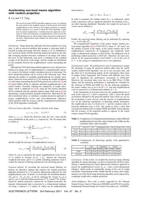
Accelerating non-local means algorithm with random projectioni and Y.T.YangThe non-local means (NLM)algorithm suppresses noise via replacing the noisy pixel by the weighted average of all the pixels with similar neighbourhood vectors.However,the weights calculation is computa-tionally expensive,as a result of which the NLM algorithm is quite slow for practical applications.A random projection approach is intro-duced to reduce the dimension of neighbourhood vectors used in the NLM filtering process,which yields a faster and more accurate denois-ing effect.Experimental results illustrate the effectiveness of the pro-posed method.Introduction:Image denoising,although it has been studied over a long time,is still an unsolved problem that remains a wide-open field of research in image processing.Recently,Buades et al.[1]established a new non-local means (NLM)denoising framework based on the idea that averaging repeated structures contained in an image will reduce the noise.In this framework,each pixel is estimated as the weighted average of all the pixels in the image,and the weights are determined by the similarity between the neighbourhood vectors surrounding the pixels.Although the NLM denoising method suppresses noise and preserves details in an image well,its implementation is computationally expens-ive owing to the tedious weights calculation process in denoising.The above-mentioned problem can be solved in the following ways.First,reducing the number of candidate neighbourhoods for weights calcu-lation,which has been realised in [2]by limiting the weight calculation to a sub-image surrounding the pixel being processed,moreover,[3]and [4]report further efforts to eliminate unrelated neighbourhoods in the search window.Secondly,reducing the complexity of weight calcu-lation,which is addressed in [5]by using the fast Fourier transform (FFT)combined with the summed squares image (SSI)and in [6]by introducing a multi-resolution pyramid architecture.Motivated by the above-mentioned ideas,we introduce a random projection approach to project neighbourhood vectors onto lower-dimensional subspaces,which promotes both the accuracy and the computational performance of the NLM algorithm considerably.Non-local means algorithm:Consider a discrete noisy imagey i ,j =x i ,j +n i ,j ,(i ,j )[I(1)where y i ,j ,x i ,j ,n i ,j denote the observed value,the ‘true’value and the noise perturbation at the pixel (i ,j ),respectively.The NL-means filter is written asˆxi ,j =1Z k ,l(i ,j )[ˆN d ×d (k ,l )w k ,l ,i ,j y i ,j (2)where the normalising termZ k ,l =(i ,j )[ˆNd ×d (k ,l )w k ,l ,i ,j(3)and the weight for each pair of neighbourhood vectors isw k ,l ,i ,j =exp −ˆN d ×d (k ,l )−ˆN d ×d (i ,j ) 22,ah 2(4)where ˆNd ×d (m ,n )represents the square neighbourhood vector of size d ×d centred at location (m ,n ), · 22,a denotes the Gaussian-weighted-semi-norm,and h is a global smoothing parameter used to control the amount of blurring introduced in the denoising process.Proposed method:To accelerate the non-local means filtering,we propose an alternative strategy that employs the random projection approach introduced in [7]to perform dimensional reduction for each neighbourhood vector.In detail,we recalculate the Euclidean distanceˆN d ×d (k ,l )−ˆN d ×d (i ,j ) 22,ain (4)by replacing the vectors ˆN d ×d (i ,j )and ˆNd ×d (k ,l )with lower-dimensional ones f RP [i ,j ]and f RP [k ,l ]deter-mined by random projection,respectively.In random projection,the original d -dimensional data is projected to a k -dimensional subspace via using a random k ×d matrix R ,which can be mathematicallyrepresented asf RP [·]=R k ×d ·ˆNd ×d (·)(5)In order to guarantee the random matrix R k ×d is orthogonal,whichyields a projection with no significant distortion,the elements of R k ×d are often Gaussian distributed.Thereafter,the weight for each pair of vectors can be defined asw RP k ,l ,i ,j =exp − f RP [k ,l ]−f RP[i ,j ] 22,ah 2(6)Finally,the non-local means filtering can be performed by replacingw k ,l ,i ,j in (2)with w RP k ,l ,i ,j .The computational complexity of the search window limited non-local means algorithm [2]is of O(N 2M 2d 2),where N 2,M 2and d 2are the number of pixels in the image,in the search window and in the neighbourhood,respectively.In comparison,the complexity when using a k -dimensional subspace is O(N 2M 2kd ).The additional cost in performing random projection is O(N 2kd 2).Therefore,the total com-plexity for the proposed method is O(N 2kd (M 2+d )).In the case of d ..k ,the saving of computational cost is very significant.Experimental results:We performed two sets of experiments to gauge the advantage of using the proposed method rather than the search window limited NLM algorithm:one set to test execution time,and the other set to test denoising quality.In the experiments,three types of images (Lena,Fingerprint,and Texture)with different sizes were used to implement the performance assessment in MATLAB.Moreover,the execution times were run on an IBM T61p 2.2GHz laptop,and the denoising performance is quantitatively evaluated by the criterions of PSNR and SSIM [8].For the following simulation,the search window size is set to be M ¼21,and each neighbourhood vector is projected to a k -dimensional subspace (k ¼1).In the experiments of execution time test,the neighbourhood size d took on the value of 5,7and 9,respectively.Table 1shows the speed acceleration afforded by the proposed method,from which we can see the acceleration is more obvious with the increase of neighbourhood size.In the following experiments of denoising quality assessment,the neighbourhood size d is fixed to be 7,and the variation value of Gaussian additional noise is 0.03.The results in Table 2show that our proposed method achieves higher PSNR and SSIM,which indicates that the accuracy of the proposed method is superior to the search window limited NLM algorithm.Table 1:Comparison of computational performance under differentneighbourhood sizes (the values listed in the Table are the execution times,units seconds)Table 2:Comparison of denoising quality with quantitativecriterionsConclusions:In this Letter,we recalled the non-local means filtering algorithm for image denoising;we then accelerated the NLM by intro-ducing a random projection based dimensional reduction approach toproject the neighbourhood vectors ˆNd ×d (·)onto a lower-dimensional subspace,which results in considerable savings in the cost of weight calculation.Experimental results validate that the accuracy and compu-tational cost of the NLM image denoising algorithm can be improved by computing weight after a random projection.Acknowledgments:This work is partly supported by the National Natural Science Fund of China (nos 60902080and 60725415)and the Fundamental Research Funds for Central Universities (no.72104909).ELECTRONICS LETTERS 3rd February 2011Vol.47No.3#The Institution of Engineering and Technology201116September2010doi:10.1049/el.2010.2618i and Y.T.Yang(Department of Microelectronics,Xidian University,Xi’an,People’s Republic of China)E-mail:rlai@References1Buades,A.,Coll,B.,and Morel,J.M.:‘A review of image denoising algorithms,with a new one’,Multiscale Model.Simul.SIAM Interdiscip.J.,2005,4,(2),pp.490–5302Buades,A.,Coll,B.,and Morel,J.M.:‘Denoising image sequences does not require motion estimation’.Proc.IEEE2005Int.Conf.Advanced Video and Signal Based Surveillance,Teatro Sociale,Italy,pp.70–74 3Mahmoudi,M.,and Sapiro,G.:‘Fast image and video denoising via nonlocal means of similar neighborhoods’,IEEE Signal Process.Lett., 2005,12,(12),pp.839–8424Orchard,J.,Ebrahimi,M.,and Wong,A.:‘Efficient non-local means denoising using the SVD’.Proc.2008IEEE Int.Conf.Image Processing,San Diego,CA,USA,pp.1732–17355Wang,J.,Guo,Y.W.,Ying,Y.T.,Liu,Y.L.,and Peng,Q.S.:‘Fast non-local algorithm for image denoising’.Proc.2006IEEE Int.Conf.Image Processing,Atlanta,GA USA,pp.1429–14326Karnati,V.,Uliyar,M.,and Dey,S.:‘Fast non-local algorithm for image denoising’.Proc.2008IEEE Int.Conf.Image Processing,San Diego, CA,USA,pp.3873–38767Bingham,E.,and Mannila,H.:‘Random projection in dimensional reduction:applications to image and text data’.Proc.2001ACM Int.Conf.Knowledge Discovery and Data Mining,San Francisco,CA, USA,pp.245–2508Wang,Z.,Bovik,A.C.,Sheikh,H.R.,and Simoncelli,E.P.:‘Image quality assessment:from error visibility to structural similarity’,IEEE Trans.Image Process.,2004,13,(4),pp.600–612ELECTRONICS LETTERS3rd February2011Vol.47No.3。
Fast Algorithms for Mining Association Rules

Rakesh Agrawal Ramakrishnan Srikant IBM Almaden Research Center 650 Harry Road, San Jose, CA 95120
Abstract
1 Introduction
Database mining is motivated by the decision support problem faced by most large retail organizations S+ 93]. Progress in bar-code technology has made it possible for retail organizations to collect and store massive amounts of sales data, referred to as the basket data. A record in such data typically consists of the transaction date and the items bought in the transaction. Successful organizations view such databases as important pieces of the marketing infrastructure Ass92]. They are interested in instituting information-driven marketing processes, managed by database technology, that enable marketers to develop and implement customized marketing programs and strategies Ass90]. The problem of mining association rules over basket data was introduced in AIS93b]. An example of such a rule might be that 98% of customers that purchase tires and auto accessories also get automotive services done. Finding all such rules is valuable for cross-marketing and attached mailing applications. Other applications include catalog design, add-on sales, store layout, and customer segmentation based on buying patterns. The databases involved in these applications are very large. It is imperative, therefore, to have fast algorithms for this task.
Secrets of Optical Flow Estimation and Their Principles
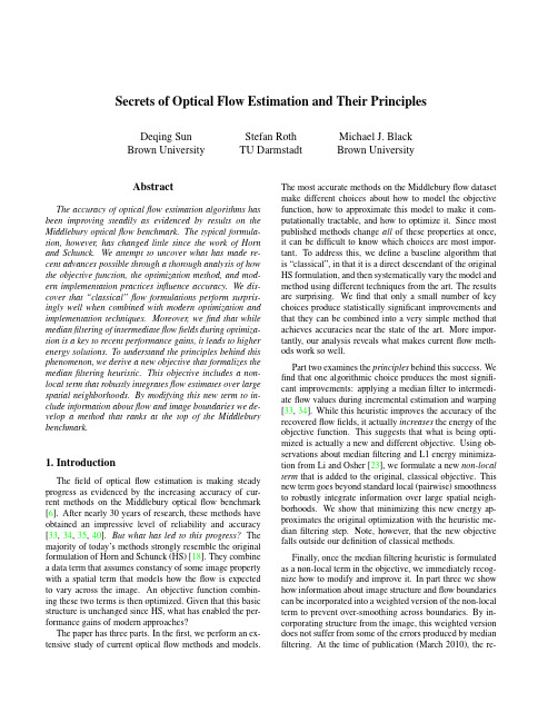
Secrets of Optical Flow Estimation and Their PrinciplesDeqing Sun Brown UniversityStefan RothTU DarmstadtMichael J.BlackBrown UniversityAbstractThe accuracy of opticalflow estimation algorithms has been improving steadily as evidenced by results on the Middlebury opticalflow benchmark.The typical formula-tion,however,has changed little since the work of Horn and Schunck.We attempt to uncover what has made re-cent advances possible through a thorough analysis of how the objective function,the optimization method,and mod-ern implementation practices influence accuracy.We dis-cover that“classical”flow formulations perform surpris-ingly well when combined with modern optimization and implementation techniques.Moreover,wefind that while medianfiltering of intermediateflowfields during optimiza-tion is a key to recent performance gains,it leads to higher energy solutions.To understand the principles behind this phenomenon,we derive a new objective that formalizes the medianfiltering heuristic.This objective includes a non-local term that robustly integratesflow estimates over large spatial neighborhoods.By modifying this new term to in-clude information aboutflow and image boundaries we de-velop a method that ranks at the top of the Middlebury benchmark.1.IntroductionThefield of opticalflow estimation is making steady progress as evidenced by the increasing accuracy of cur-rent methods on the Middlebury opticalflow benchmark [6].After nearly30years of research,these methods have obtained an impressive level of reliability and accuracy [33,34,35,40].But what has led to this progress?The majority of today’s methods strongly resemble the original formulation of Horn and Schunck(HS)[18].They combine a data term that assumes constancy of some image property with a spatial term that models how theflow is expected to vary across the image.An objective function combin-ing these two terms is then optimized.Given that this basic structure is unchanged since HS,what has enabled the per-formance gains of modern approaches?The paper has three parts.In thefirst,we perform an ex-tensive study of current opticalflow methods and models.The most accurate methods on the Middleburyflow dataset make different choices about how to model the objective function,how to approximate this model to make it com-putationally tractable,and how to optimize it.Since most published methods change all of these properties at once, it can be difficult to know which choices are most impor-tant.To address this,we define a baseline algorithm that is“classical”,in that it is a direct descendant of the original HS formulation,and then systematically vary the model and method using different techniques from the art.The results are surprising.Wefind that only a small number of key choices produce statistically significant improvements and that they can be combined into a very simple method that achieves accuracies near the state of the art.More impor-tantly,our analysis reveals what makes currentflow meth-ods work so well.Part two examines the principles behind this success.We find that one algorithmic choice produces the most signifi-cant improvements:applying a medianfilter to intermedi-ateflow values during incremental estimation and warping [33,34].While this heuristic improves the accuracy of the recoveredflowfields,it actually increases the energy of the objective function.This suggests that what is being opti-mized is actually a new and different ing ob-servations about medianfiltering and L1energy minimiza-tion from Li and Osher[23],we formulate a new non-local term that is added to the original,classical objective.This new term goes beyond standard local(pairwise)smoothness to robustly integrate information over large spatial neigh-borhoods.We show that minimizing this new energy ap-proximates the original optimization with the heuristic me-dianfiltering step.Note,however,that the new objective falls outside our definition of classical methods.Finally,once the medianfiltering heuristic is formulated as a non-local term in the objective,we immediately recog-nize how to modify and improve it.In part three we show how information about image structure andflow boundaries can be incorporated into a weighted version of the non-local term to prevent over-smoothing across boundaries.By in-corporating structure from the image,this weighted version does not suffer from some of the errors produced by median filtering.At the time of publication(March2010),the re-sulting approach is ranked1st in both angular and end-point errors in the Middlebury evaluation.In summary,the contributions of this paper are to(1)an-alyze currentflow models and methods to understand which design choices matter;(2)formulate and compare several classical objectives descended from HS using modern meth-ods;(3)formalize one of the key heuristics and derive a new objective function that includes a non-local term;(4)mod-ify this new objective to produce a state-of-the-art method. In doing this,we provide a“recipe”for others studying op-ticalflow that can guide their design choices.Finally,to en-able comparison and further innovation,we provide a public M ATLAB implementation[1].2.Previous WorkIt is important to separately analyze the contributions of the objective function that defines the problem(the model) and the optimization algorithm and implementation used to minimize it(the method).The HS formulation,for example, has long been thought to be highly inaccurate.Barron et al.[7]reported an average angular error(AAE)of~30degrees on the“Yosemite”sequence.This confounds the objective function with the particular optimization method proposed by Horn and Schunck1.When optimized with today’s meth-ods,the HS objective achieves surprisingly competitive re-sults despite the expected over-smoothing and sensitivity to outliers.Models:The global formulation of opticalflow intro-duced by Horn and Schunck[18]relies on both brightness constancy and spatial smoothness assumptions,but suffers from the fact that the quadratic formulation is not robust to outliers.Black and Anandan[10]addressed this by re-placing the quadratic error function with a robust formula-tion.Subsequently,many different robust functions have been explored[12,22,31]and it remains unclear which is best.We refer to all these spatially-discrete formulations derived from HS as“classical.”We systematically explore variations in the formulation and optimization of these ap-proaches.The surprise is that the classical model,appropri-ately implemented,remains very competitive.There are many formulations beyond the classical ones that we do not consider here.Significant ones use oriented smoothness[25,31,33,40],rigidity constraints[32,33], or image segmentation[9,21,41,37].While they deserve similar careful consideration,we expect many of our con-clusions to carry forward.Note that one can select among a set of models for a given sequence[4],instead offinding a “best”model for all the sequences.Methods:Many of the implementation details that are thought to be important date back to the early days of op-1They noted that the correct way to optimize their objective is by solv-ing a system of linear equations as is common today.This was impractical on the computers of the day so they used a heuristic method.ticalflow.Current best practices include coarse-to-fine es-timation to deal with large motions[8,13],texture decom-position[32,34]or high-orderfilter constancy[3,12,16, 22,40]to reduce the influence of lighting changes,bicubic interpolation-based warping[22,34],temporal averaging of image derivatives[17,34],graduated non-convexity[11]to minimize non-convex energies[10,31],and medianfilter-ing after each incremental estimation step to remove outliers [34].This medianfiltering heuristic is of particular interest as it makes non-robust methods more robust and improves the accuracy of all methods we tested.The effect on the objec-tive function and the underlying reason for its success have not previously been analyzed.Least median squares estima-tion can be used to robustly reject outliers inflow estimation [5],but previous work has focused on the data term.Related to medianfiltering,and our new non-local term, is the use of bilateralfiltering to prevent smoothing across motion boundaries[36].The approach separates a varia-tional method into twofiltering update stages,and replaces the original anisotropic diffusion process with multi-cue driven bilateralfiltering.As with medianfiltering,the bi-lateralfiltering step changes the original energy function.Models that are formulated with an L1robust penalty are often coupled with specialized total variation(TV)op-timization methods[39].Here we focus on generic opti-mization methods that can apply to any model andfind they perform as well as reported results for specialized methods.Despite recent algorithmic advances,there is a lack of publicly available,easy to use,and accurateflow estimation software.The GPU4Vision project[2]has made a substan-tial effort to change this and provides executablefiles for several accurate methods[32,33,34,35].The dependence on the GPU and the lack of source code are limitations.We hope that our public M ATLAB code will not only help in un-derstanding the“secrets”of opticalflow,but also let others exploit opticalflow as a useful tool in computer vision and relatedfields.3.Classical ModelsWe write the“classical”opticalflow objective function in its spatially discrete form asE(u,v)=∑i,j{ρD(I1(i,j)−I2(i+u i,j,j+v i,j))(1)+λ[ρS(u i,j−u i+1,j)+ρS(u i,j−u i,j+1)+ρS(v i,j−v i+1,j)+ρS(v i,j−v i,j+1)]}, where u and v are the horizontal and vertical components of the opticalflowfield to be estimated from images I1and I2,λis a regularization parameter,andρD andρS are the data and spatial penalty functions.We consider three different penalty functions:(1)the quadratic HS penaltyρ(x)=x2;(2)the Charbonnier penaltyρ(x)=√x2+ 2[13],a dif-ferentiable variant of the L1norm,the most robust convexfunction;and(3)the Lorentzianρ(x)=log(1+x22σ2),whichis a non-convex robust penalty used in[10].Note that this classical model is related to a standard pairwise Markov randomfield(MRF)based on a4-neighborhood.In the remainder of this section we define a baseline method using several techniques from the literature.This is not the“best”method,but includes modern techniques and will be used for comparison.We only briefly describe the main choices,which are explored in more detail in the following section and the cited references,especially[30].Quantitative results are presented throughout the remain-der of the text.In all cases we report the average end-point error(EPE)on the Middlebury training and test sets,de-pending on the experiment.Given the extensive nature of the evaluation,only average results are presented in the main body,while the details for each individual sequence are given in[30].3.1.Baseline methodsTo gain robustness against lighting changes,we follow [34]and apply the Rudin-Osher-Fatemi(ROF)structure texture decomposition method[28]to pre-process the in-put sequences and linearly combine the texture and struc-ture components(in the proportion20:1).The parameters are set according to[34].Optimization is performed using a standard incremental multi-resolution technique(e.g.[10,13])to estimateflow fields with large displacements.The opticalflow estimated at a coarse level is used to warp the second image toward thefirst at the nextfiner level,and aflow increment is cal-culated between thefirst image and the warped second im-age.The standard deviation of the Gaussian anti-aliasingfilter is set to be1√2d ,where d denotes the downsamplingfactor.Each level is recursively downsampled from its near-est lower level.In building the pyramid,the downsampling factor is not critical as pointed out in the next section and here we use the settings in[31],which uses a factor of0.8 in thefinal stages of the optimization.We adaptively de-termine the number of pyramid levels so that the top level has a width or height of around20to30pixels.At each pyramid level,we perform10warping steps to compute the flow increment.At each warping step,we linearize the data term,whichinvolves computing terms of the type∂∂x I2(i+u k i,j,j+v k i,j),where∂/∂x denotes the partial derivative in the horizon-tal direction,u k and v k denote the currentflow estimate at iteration k.As suggested in[34],we compute the deriva-tives of the second image using the5-point derivativefilter1 12[−180−81],and warp the second image and its deriva-tives toward thefirst using the currentflow estimate by bicu-bic interpolation.We then compute the spatial derivatives ofAvg.Rank Avg.EPEClassic-C14.90.408HS24.60.501Classic-L19.80.530HS[31]35.10.872BA(Classic-L)[31]30.90.746Adaptive[33]11.50.401Complementary OF[40]10.10.485Table1.Models.Average rank and end-point error(EPE)on the Middlebury test set using different penalty functions.Two current methods are included for comparison.thefirst image,average with the warped derivatives of the second image(c.f.[17]),and use this in place of∂I2∂x.For pixels moving out of the image boundaries,we set both their corresponding temporal and spatial derivatives to zero.Af-ter each warping step,we apply a5×5medianfilter to the newly computedflowfield to remove outliers[34].For the Charbonnier(Classic-C)and Lorentzian (Classic-L)penalty function,we use a graduated non-convexity(GNC)scheme[11]as described in[31]that lin-early combines a quadratic objective with a robust objective in varying proportions,from fully quadratic to fully robust. Unlike[31],a single regularization weightλis used for both the quadratic and the robust objective functions.3.2.Baseline resultsThe regularization parameterλis selected among a set of candidate values to achieve the best average end-point error (EPE)on the Middlebury training set.For the Charbonnier penalty function,the candidate set is[1,3,5,8,10]and 5is optimal.The Charbonnier penalty uses =0.001for both the data and the spatial term in Eq.(1).The Lorentzian usesσ=1.5for the data term,andσ=0.03for the spa-tial term.These parameters arefixed throughout the exper-iments,except where mentioned.Table1summarizes the EPE results of the basic model with three different penalty functions on the Middlebury test set,along with the two top performers at the time of publication(considering only published papers).The clas-sic formulations with two non-quadratic penalty functions (Classic-C)and(Classic-L)achieve competitive results de-spite their simplicity.The baseline optimization of HS and BA(Classic-L)results in significantly better accuracy than previously reported for these models[31].Note that the analysis also holds for the training set(Table2).At the time of publication,Classic-C ranks13th in av-erage EPE and15th in AAE in the Middlebury benchmark despite its simplicity,and it serves as the baseline below.It is worth noting that the spatially discrete MRF formulation taken here is competitive with variational methods such as [33].Moreover,our baseline implementation of HS has a lower average EPE than many more sophisticated methods.Avg.EPE significance p-value Classic-C0.298——HS0.38410.0078Classic-L0.31910.0078Classic-C-brightness0.28800.9453HS-brightness0.38710.0078Classic-L-brightness0.32500.2969Gradient0.30500.4609Table2.Pre-Processing.Average end-point error(EPE)on the Middlebury training set for the baseline method(Classic-C)using different pre-processing techniques.Significance is always with respect to Classic-C.4.Secrets ExploredWe evaluate a range of variations from the baseline ap-proach that have appeared in the literature,in order to illu-minate which may be of importance.This analysis is per-formed on the Middlebury training set by changing only one property at a time.Statistical significance is determined using a Wilcoxon signed rank test between each modified method and the baseline Classic-C;a p value less than0.05 indicates a significant difference.Pre-Processing.For each method,we optimize the regu-larization parameterλfor the training sequences and report the results in Table2.The baseline uses a non-linear pre-filtering of the images to reduce the influence of illumina-tion changes[34].Table2shows the effect of removing this and using a standard brightness constancy model(*-brightness).Classic-C-brightness actually achieves lower EPE on the training set than Classic-C but significantly lower accuracy on the test set:Classic-C-brightness= 0.726,HS-brightness=0.759,and Classic-L-brightness =0.603–see Table1for comparison.This disparity sug-gests overfitting is more severe for the brightness constancy assumption.Gradient only imposes constancy of the gra-dient vector at each pixel as proposed in[12](i.e.it robustly penalizes Euclidean distance between image gradients)and has similar performance in both training and test sets(c.f. Table8).See[30]for results of more alternatives. Secrets:Some form of imagefiltering is useful but simple derivative constancy is nearly as good as the more sophisti-cated texture decomposition method.Coarse-to-fine estimation and GNC.We vary the number of warping steps per pyramid level andfind that3warping steps gives similar results as using10(Table3).For the GNC scheme,[31]uses a downsampling factor of0.8for non-convex optimization.A downsampling factor of0.5 (Down-0.5),however,has nearly identical performance Removing the GNC step for the Charbonnier penalty function(w/o GNC)results in higher EPE on most se-quences and higher energy on all sequences(Table4).This suggests that the GNC method is helpful even for the con-vex Charbonnier penalty function due to the nonlinearity ofAvg.EPE significance p-value Classic-C0.298——3warping steps0.30400.9688Down-0.50.2980 1.0000w/o GNC0.35400.1094Bilinear0.30200.1016w/o TA VG0.30600.1562Central derivativefilter0.30000.72667-point derivativefilter[13]0.30200.3125Bicubic-II0.29010.0391GC-0.45(λ=3)0.29210.0156GC-0.25(λ=0.7)0.2980 1.0000MF3×30.30500.1016MF7×70.30500.56252×MF0.3000 1.00005×MF0.30500.6875w/o MF0.35210.0078Classic++0.28510.0078 Table3.Model and Methods.Average end-point error(EPE)on the Middlebury training set for the baseline method(Classic-C) using different algorithm and modelingchoices.Figure1.Different penalty functions for the spatial terms:Char-bonnier( =0.001),generalized Charbonnier(a=0.45and a=0.25),and Lorentzian(σ=0.03).the data term.Secrets:The downsampling factor does not matter when using a convex penalty;a standard factor of0.5isfine. Some form of GNC is useful even for a convex robust penalty like Charbonnier because of the nonlinear data term. Interpolation method and derivatives.Wefind that bicu-bic interpolation is more accurate than bilinear(Table3, Bilinear),as already reported in previous work[34].Re-moving temporal averaging of the gradients(w/o TA VG), using Central differencefilters,or using a7-point deriva-tivefilter[13]all reduce accuracy compared to the base-line,but not significantly.The M ATLAB built-in function interp2is based on cubic convolution approximation[20]. The spline-based interpolation scheme[26]is consistently better(Bicubic-II).See[30]for more discussions. Secrets:Use spline-based bicubic interpolation with a5-pointfilter.Temporal averaging of the derivatives is proba-bly worthwhile for a small computational expense. Penalty functions.Wefind that the convex Charbonnier penalty performs better than the more robust,non-convex Lorentzian on both the training and test sets.One reason might be that non-convex functions are more difficult to op-timize,causing the optimization scheme tofind a poor local(a)With medianfiltering(b)Without medianfilteringFigure2.Estimatedflowfields on sequence“RubberWhale”using Classic-C with and without(w/o MF)the medianfiltering step. Color coding as in[6].(a)(w/MF)energy502,387and(b)(w/o MF)energy449,290.The medianfiltering step helps reach a so-lution free from outliers but with a higher energy.optimum.We investigate a generalized Charbonnier penalty functionρ(x)=(x2+ 2)a that is equal to the Charbon-nier penalty when a=0.5,and non-convex when a<0.5 (see Figure1).We optimize the regularization parameterλagain.Wefind a slightly non-convex penalty with a=0.45 (GC-0.45)performs consistently better than the Charbon-nier penalty,whereas more non-convex penalties(GC-0.25 with a=0.25)show no improvement.Secrets:The less-robust Charbonnier is preferable to the Lorentzian and a slightly non-convex penalty function(GC-0.45)is better still.Medianfiltering.The baseline5×5medianfilter(MF 5×5)is better than both MF3×3[34]and MF7×7but the difference is not significant(Table3).When we perform5×5medianfiltering twice(2×MF)orfive times(5×MF)per warping step,the results are worse.Finally,removing the medianfiltering step(w/o MF)makes the computedflow significantly less accurate with larger outliers as shown in Table3and Figure2.Secrets:Medianfiltering the intermediateflow results once after every warping iteration is the single most important secret;5×5is a goodfilter size.4.1.Best PracticesCombining the analysis above into a single approach means modifying the baseline to use the slightly non-convex generalized Charbonnier and the spline-based bicu-bic interpolation.This leads to a statistically significant improvement over the baseline(Table3,Classic++).This method is directly descended from HS and BA,yet updated with the current best optimization practices known to us. This simple method ranks9th in EPE and12th in AAE on the Middlebury test set.5.Models Underlying Median FilteringOur analysis reveals the practical importance of median filtering during optimization to denoise theflowfield.We ask whether there is a principle underlying this heuristic?One interesting observation is thatflowfields obtained with medianfiltering have substantially higher energy than those without(Table4and Figure2).If the medianfilter is helping to optimize the objective,it should lead to lower energies.Higher energies and more accurate estimates sug-gest that incorporating medianfiltering changes the objec-tive function being optimized.The insight that follows from this is that the medianfil-tering heuristic is related to the minimization of an objective function that differs from the classical one.In particular the optimization of Eq.(1),with interleaved medianfiltering, approximately minimizesE A(u,v,ˆu,ˆv)=(2)∑i,j{ρD(I1(i,j)−I2(i+u i,j,j+v i,j))+λ[ρS(u i,j−u i+1,j)+ρS(u i,j−u i,j+1)+ρS(v i,j−v i+1,j)+ρS(v i,j−v i,j+1)]}+λ2(||u−ˆu||2+||v−ˆv||2)+∑i,j∑(i ,j )∈N i,jλ3(|ˆu i,j−ˆu i ,j |+|ˆv i,j−ˆv i ,j |),whereˆu andˆv denote an auxiliaryflowfield,N i,j is the set of neighbors of pixel(i,j)in a possibly large area andλ2 andλ3are scalar weights.The term in braces is the same as theflow energy from Eq.(1),while the last term is new. This non-local term[14,15]imposes a particular smooth-ness assumption within a specified region of the auxiliary flowfieldˆu,ˆv2.Here we take this term to be a5×5rectan-gular region to match the size of the medianfilter in Classic-C.A third(coupling)term encouragesˆu,ˆv and u,v to be the same(c.f.[33,39]).The connection to medianfiltering(as a denoising method)derives from the fact that there is a direct relation-ship between the median and L1minimization.Consider a simplified version of Eq.(2)with just the coupling and non-local terms,where E(ˆu)=λ2||u−ˆu||2+∑i,j∑(i ,j )∈N i,jλ3|ˆu i,j−ˆu i ,j |.(3)While minimizing this is similar to medianfiltering u,there are two differences.First,the non-local term minimizes the L1distance between the central value and allflow values in its neighborhood except itself.Second,Eq.(3)incorpo-rates information about the data term through the coupling equation;medianfiltering theflow ignores the data term.The formal connection between Eq.(3)and medianfil-tering3is provided by Li and Osher[23]who show that min-2Bruhn et al.[13]also integrated information over a local region in a global method but did so for the data term.3Hsiao et al.[19]established the connection in a slightly different way.Classic-C 0.5890.7480.8660.502 1.816 2.317 1.126 1.424w/o GNC 0.5930.7500.8700.506 1.845 2.518 1.142 1.465w/o MF0.5170.7010.6680.449 1.418 1.830 1.066 1.395Table 4.Eq.(1)energy (×106)for the optical flow fields computed on the Middlebury training set .Note that Classic-C uses graduated non-convexity (GNC),which reduces the energy,and median filtering,which increases it.imizing Eq.(3)is related to a different median computationˆu (k +1)i,j=median (Neighbors (k )∪Data)(4)where Neighbors (k )={ˆu (k )i ,j }for (i ,j )∈N i,j and ˆu (0)=u as well as Data ={u i,j ,u i,j ±λ3λ2,u i,j±2λ3λ2···,u i,j ±|N i,j |λ32λ2},where |N i,j |denotes the (even)number of neighbors of (i,j ).Note that the set of “data”values is balanced with an equal number of elements on either side of the value u i,j and that information about the data term is included through u i,j .Repeated application of Eq.(4)converges rapidly [23].Observe that,as λ3/λ2increases,the weighted data val-ues on either side of u i,j move away from the values of Neighbors and cancel each other out.As this happens,Eq.(4)approximates the median at the first iterationˆu (1)i,j ≈median (Neighbors (0)∪{u i,j }).(5)Eq.(2)thus combines the original objective with an ap-proximation to the median,the influence of which is con-trolled by λ3/λ2.Note in practice the weight λ2on thecoupling term is usually small or is steadily increased from small values [34,39].We optimize the new objective (2)by alternately minimizingE O (u ,v )=∑i,jρD (I 1(i,j )−I 2(i +u i,j ,j +v i,j ))+λ[ρS (u i,j −u i +1,j )+ρS (u i,j −u i,j +1)+ρS (v i,j −v i +1,j )+ρS (v i,j −v i,j +1)]+λ2(||u −ˆu ||2+||v −ˆv ||2)(6)andE M (ˆu ,ˆv )=λ2(||u −ˆu ||2+||v −ˆv ||2)(7)+∑i,j ∑(i ,j )∈N i,jλ3(|ˆu i,j −ˆu i ,j |+|ˆv i,j −ˆv i ,j |).Note that an alternative formulation would drop the cou-pling term and impose the non-local term directly on u and v .We find that optimization of the coupled set of equations is superior in terms of EPE performance.The alternating optimization strategy first holds ˆu ,ˆv fixed and minimizes Eq.(6)w.r.t.u ,v .Then,with u ,v fixed,we minimize Eq.(7)w.r.t.ˆu ,ˆv .Note that Eqs.(3)andAvg.EPE significancep -value Classic-C0.298——Classic-C-A0.30500.8125Table 5.Average end-point error (EPE)on the Middlebury train-ing set is shown for the new model with alternating optimization (Classic-C-A ).(7)can be minimized by repeated application of Eq.(4);weuse this approach with 5iterations.We perform 10steps of alternating optimizations at every pyramid level and change λ2logarithmically from 10−4to 102.During the first and second GNC stages,we set u ,v to be ˆu ,ˆv after every warp-ing step (this step helps reach solutions with lower energy and EPE [30]).In the end,we take ˆu ,ˆv as the final flow field estimate.The other parameters are λ=5,λ3=1.Alternatingly optimizing this new objective function (Classic-C-A )leads to similar results as the baseline Classic-C (Table 5).We also compare the energy of these solutions using the new objective and find the alternat-ing optimization produces the lowest energy solutions,as shown in Table 6.To do so,we set both the flow field u ,v and the auxiliary flow field ˆu ,ˆv to be the same in Eq.(2).In summary,we show that the heuristic median filter-ing step in Classic-C can now be viewed as energy min-imization of a new objective with a non-local term.The explicit formulation emphasizes the value of robustly inte-grating information over large neighborhoods and enables the improved model described below.6.Improved ModelBy formalizing the median filtering heuristic as an ex-plicit objective function,we can find ways to improve it.While median filtering in a large neighborhood has advan-tages as we have seen,it also has problems.A neighborhood centered on a corner or thin structure is dominated by the surround and computing the median results in oversmooth-ing as illustrated in Figure 3(a).Examining the non-local term suggests a solution.For a given pixel,if we know which other pixels in the area be-long to the same surface,we can weight them more highly.The modification to the objective function is achieved by introducing a weight into the non-local term [14,15]:∑i,j ∑(i ,j )∈N i,jw i,j,i ,j (|ˆu i,j −ˆu i ,j |+|ˆv i,j −ˆv i ,j |),(8)where w i,j,i ,j represents how likely pixel i ,j is to belongto the same surface as i,j .。
时间序列分类问题的算法比较
8期杨一鸣等t时问序列分类问题的算{击比较1265在今后的工作中,我们将会把具体的分类算法[II]考虑进去来做进一步的预处理,考虑怎样的属性组合可以更好地提高我们算法分类的性能.我们也计划把算法运用到其他的多维序列数据集中.参考文献口]Itaku珀EM川mumpre山ctlonr姻ldualpnnclpleappIled8peech舢gnIlIon.IEEET埘mctIonsAcoustlcsSp∞chSlgn且1ProcesB(ASSP).1975t23(1)I52—72[2]Kruska¨JB,LIberIlI皿M.TheBymmetnctImewarm“gal—gonthm,Fromcontl删oustod15crete//T吼eWarps,St“ngEdit8andMacromolecul凹.Addl∞n,1983[3]M”rBc.Rabln盯L,Rosenebe79A.Pcdotradeoffs.ndynaIⅡicn㈣rPmgalgorithmsfor1solatedwordrecog—m“0tI.IEEETfan5actIonsonA洲t瑚SpeechSIgnalProce3s(ASSP)。
1980.28(6):623—635[4]&rⅡdtD,alffordJ.usl“gdynamlctl眦wafplIlgt。
hndpattⅢmt雌鲫es//ProceedlElgso“hAAAI·94work—shopKnowledgenscoveryDataba8e8.s曲ttle,wAtUSA.1994:229—248[5]AachJ,chufchG.A119n1“ggenecxp心5slontImc8盯le8Wltht帅e珊rpillgdgonthm8.Blmnf蝴tl∞,2001.17:495—508[6]白laIIiEG,P。
naAtB聃eIhG,T咖lM,Muzzupappas.Plcruz西F。
交通流
Network impacts of a road capacity reduction:Empirical analysisand model predictionsDavid Watling a ,⇑,David Milne a ,Stephen Clark baInstitute for Transport Studies,University of Leeds,Woodhouse Lane,Leeds LS29JT,UK b Leeds City Council,Leonardo Building,2Rossington Street,Leeds LS28HD,UKa r t i c l e i n f o Article history:Received 24May 2010Received in revised form 15July 2011Accepted 7September 2011Keywords:Traffic assignment Network models Equilibrium Route choice Day-to-day variabilitya b s t r a c tIn spite of their widespread use in policy design and evaluation,relatively little evidencehas been reported on how well traffic equilibrium models predict real network impacts.Here we present what we believe to be the first paper that together analyses the explicitimpacts on observed route choice of an actual network intervention and compares thiswith the before-and-after predictions of a network equilibrium model.The analysis isbased on the findings of an empirical study of the travel time and route choice impactsof a road capacity reduction.Time-stamped,partial licence plates were recorded across aseries of locations,over a period of days both with and without the capacity reduction,and the data were ‘matched’between locations using special-purpose statistical methods.Hypothesis tests were used to identify statistically significant changes in travel times androute choice,between the periods of days with and without the capacity reduction.A trafficnetwork equilibrium model was then independently applied to the same scenarios,and itspredictions compared with the empirical findings.From a comparison of route choice pat-terns,a particularly influential spatial effect was revealed of the parameter specifying therelative values of distance and travel time assumed in the generalised cost equations.When this parameter was ‘fitted’to the data without the capacity reduction,the networkmodel broadly predicted the route choice impacts of the capacity reduction,but with othervalues it was seen to perform poorly.The paper concludes by discussing the wider practicaland research implications of the study’s findings.Ó2011Elsevier Ltd.All rights reserved.1.IntroductionIt is well known that altering the localised characteristics of a road network,such as a planned change in road capacity,will tend to have both direct and indirect effects.The direct effects are imparted on the road itself,in terms of how it can deal with a given demand flow entering the link,with an impact on travel times to traverse the link at a given demand flow level.The indirect effects arise due to drivers changing their travel decisions,such as choice of route,in response to the altered travel times.There are many practical circumstances in which it is desirable to forecast these direct and indirect impacts in the context of a systematic change in road capacity.For example,in the case of proposed road widening or junction improvements,there is typically a need to justify econom-ically the required investment in terms of the benefits that will likely accrue.There are also several examples in which it is relevant to examine the impacts of road capacity reduction .For example,if one proposes to reallocate road space between alternative modes,such as increased bus and cycle lane provision or a pedestrianisation scheme,then typically a range of alternative designs exist which may differ in their ability to accommodate efficiently the new traffic and routing patterns.0965-8564/$-see front matter Ó2011Elsevier Ltd.All rights reserved.doi:10.1016/j.tra.2011.09.010⇑Corresponding author.Tel.:+441133436612;fax:+441133435334.E-mail address:d.p.watling@ (D.Watling).168 D.Watling et al./Transportation Research Part A46(2012)167–189Through mathematical modelling,the alternative designs may be tested in a simulated environment and the most efficient selected for implementation.Even after a particular design is selected,mathematical models may be used to adjust signal timings to optimise the use of the transport system.Road capacity may also be affected periodically by maintenance to essential services(e.g.water,electricity)or to the road itself,and often this can lead to restricted access over a period of days and weeks.In such cases,planning authorities may use modelling to devise suitable diversionary advice for drivers,and to plan any temporary changes to traffic signals or priorities.Berdica(2002)and Taylor et al.(2006)suggest more of a pro-ac-tive approach,proposing that models should be used to test networks for potential vulnerability,before any reduction mate-rialises,identifying links which if reduced in capacity over an extended period1would have a substantial impact on system performance.There are therefore practical requirements for a suitable network model of travel time and route choice impacts of capac-ity changes.The dominant method that has emerged for this purpose over the last decades is clearly the network equilibrium approach,as proposed by Beckmann et al.(1956)and developed in several directions since.The basis of using this approach is the proposition of what are believed to be‘rational’models of behaviour and other system components(e.g.link perfor-mance functions),with site-specific data used to tailor such models to particular case studies.Cross-sectional forecasts of network performance at specific road capacity states may then be made,such that at the time of any‘snapshot’forecast, drivers’route choices are in some kind of individually-optimum state.In this state,drivers cannot improve their route selec-tion by a unilateral change of route,at the snapshot travel time levels.The accepted practice is to‘validate’such models on a case-by-case basis,by ensuring that the model—when supplied with a particular set of parameters,input network data and input origin–destination demand data—reproduces current mea-sured mean link trafficflows and mean journey times,on a sample of links,to some degree of accuracy(see for example,the practical guidelines in TMIP(1997)and Highways Agency(2002)).This kind of aggregate level,cross-sectional validation to existing conditions persists across a range of network modelling paradigms,ranging from static and dynamic equilibrium (Florian and Nguyen,1976;Leonard and Tough,1979;Stephenson and Teply,1984;Matzoros et al.,1987;Janson et al., 1986;Janson,1991)to micro-simulation approaches(Laird et al.,1999;Ben-Akiva et al.,2000;Keenan,2005).While such an approach is plausible,it leaves many questions unanswered,and we would particularly highlight two: 1.The process of calibration and validation of a network equilibrium model may typically occur in a cycle.That is to say,having initially calibrated a model using the base data sources,if the subsequent validation reveals substantial discrep-ancies in some part of the network,it is then natural to adjust the model parameters(including perhaps even the OD matrix elements)until the model outputs better reflect the validation data.2In this process,then,we allow the adjustment of potentially a large number of network parameters and input data in order to replicate the validation data,yet these data themselves are highly aggregate,existing only at the link level.To be clear here,we are talking about a level of coarseness even greater than that in aggregate choice models,since we cannot even infer from link-level data the aggregate shares on alternative routes or OD movements.The question that arises is then:how many different combinations of parameters and input data values might lead to a similar link-level validation,and even if we knew the answer to this question,how might we choose between these alternative combinations?In practice,this issue is typically neglected,meaning that the‘valida-tion’is a rather weak test of the model.2.Since the data are cross-sectional in time(i.e.the aim is to reproduce current base conditions in equilibrium),then in spiteof the large efforts required in data collection,no empirical evidence is routinely collected regarding the model’s main purpose,namely its ability to predict changes in behaviour and network performance under changes to the network/ demand.This issue is exacerbated by the aggregation concerns in point1:the‘ambiguity’in choosing appropriate param-eter values to satisfy the aggregate,link-level,base validation strengthens the need to independently verify that,with the selected parameter values,the model responds reliably to changes.Although such problems–offitting equilibrium models to cross-sectional data–have long been recognised by practitioners and academics(see,e.g.,Goodwin,1998), the approach described above remains the state-of-practice.Having identified these two problems,how might we go about addressing them?One approach to thefirst problem would be to return to the underlying formulation of the network model,and instead require a model definition that permits analysis by statistical inference techniques(see for example,Nakayama et al.,2009).In this way,we may potentially exploit more information in the variability of the link-level data,with well-defined notions(such as maximum likelihood)allowing a systematic basis for selection between alternative parameter value combinations.However,this approach is still using rather limited data and it is natural not just to question the model but also the data that we use to calibrate and validate it.Yet this is not altogether straightforward to resolve.As Mahmassani and Jou(2000) remarked:‘A major difficulty...is obtaining observations of actual trip-maker behaviour,at the desired level of richness, simultaneously with measurements of prevailing conditions’.For this reason,several authors have turned to simulated gaming environments and/or stated preference techniques to elicit information on drivers’route choice behaviour(e.g. 1Clearly,more sporadic and less predictable reductions in capacity may also occur,such as in the case of breakdowns and accidents,and environmental factors such as severe weather,floods or landslides(see for example,Iida,1999),but the responses to such cases are outside the scope of the present paper. 2Some authors have suggested more systematic,bi-level type optimization processes for thisfitting process(e.g.Xu et al.,2004),but this has no material effect on the essential points above.D.Watling et al./Transportation Research Part A46(2012)167–189169 Mahmassani and Herman,1990;Iida et al.,1992;Khattak et al.,1993;Vaughn et al.,1995;Wardman et al.,1997;Jou,2001; Chen et al.,2001).This provides potentially rich information for calibrating complex behavioural models,but has the obvious limitation that it is based on imagined rather than real route choice situations.Aside from its common focus on hypothetical decision situations,this latter body of work also signifies a subtle change of emphasis in the treatment of the overall network calibration problem.Rather than viewing the network equilibrium calibra-tion process as a whole,the focus is on particular components of the model;in the cases above,the focus is on that compo-nent concerned with how drivers make route decisions.If we are prepared to make such a component-wise analysis,then certainly there exists abundant empirical evidence in the literature,with a history across a number of decades of research into issues such as the factors affecting drivers’route choice(e.g.Wachs,1967;Huchingson et al.,1977;Abu-Eisheh and Mannering,1987;Duffell and Kalombaris,1988;Antonisse et al.,1989;Bekhor et al.,2002;Liu et al.,2004),the nature of travel time variability(e.g.Smeed and Jeffcoate,1971;Montgomery and May,1987;May et al.,1989;McLeod et al., 1993),and the factors affecting trafficflow variability(Bonsall et al.,1984;Huff and Hanson,1986;Ribeiro,1994;Rakha and Van Aerde,1995;Fox et al.,1998).While these works provide useful evidence for the network equilibrium calibration problem,they do not provide a frame-work in which we can judge the overall‘fit’of a particular network model in the light of uncertainty,ambient variation and systematic changes in network attributes,be they related to the OD demand,the route choice process,travel times or the network data.Moreover,such data does nothing to address the second point made above,namely the question of how to validate the model forecasts under systematic changes to its inputs.The studies of Mannering et al.(1994)and Emmerink et al.(1996)are distinctive in this context in that they address some of the empirical concerns expressed in the context of travel information impacts,but their work stops at the stage of the empirical analysis,without a link being made to net-work prediction models.The focus of the present paper therefore is both to present thefindings of an empirical study and to link this empirical evidence to network forecasting models.More recently,Zhu et al.(2010)analysed several sources of data for evidence of the traffic and behavioural impacts of the I-35W bridge collapse in Minneapolis.Most pertinent to the present paper is their location-specific analysis of linkflows at 24locations;by computing the root mean square difference inflows between successive weeks,and comparing the trend for 2006with that for2007(the latter with the bridge collapse),they observed an apparent transient impact of the bridge col-lapse.They also showed there was no statistically-significant evidence of a difference in the pattern offlows in the period September–November2007(a period starting6weeks after the bridge collapse),when compared with the corresponding period in2006.They suggested that this was indicative of the length of a‘re-equilibration process’in a conceptual sense, though did not explicitly compare their empiricalfindings with those of a network equilibrium model.The structure of the remainder of the paper is as follows.In Section2we describe the process of selecting the real-life problem to analyse,together with the details and rationale behind the survey design.Following this,Section3describes the statistical techniques used to extract information on travel times and routing patterns from the survey data.Statistical inference is then considered in Section4,with the aim of detecting statistically significant explanatory factors.In Section5 comparisons are made between the observed network data and those predicted by a network equilibrium model.Finally,in Section6the conclusions of the study are highlighted,and recommendations made for both practice and future research.2.Experimental designThe ultimate objective of the study was to compare actual data with the output of a traffic network equilibrium model, specifically in terms of how well the equilibrium model was able to correctly forecast the impact of a systematic change ap-plied to the network.While a wealth of surveillance data on linkflows and travel times is routinely collected by many local and national agencies,we did not believe that such data would be sufficiently informative for our purposes.The reason is that while such data can often be disaggregated down to small time step resolutions,the data remains aggregate in terms of what it informs about driver response,since it does not provide the opportunity to explicitly trace vehicles(even in aggre-gate form)across more than one location.This has the effect that observed differences in linkflows might be attributed to many potential causes:it is especially difficult to separate out,say,ambient daily variation in the trip demand matrix from systematic changes in route choice,since both may give rise to similar impacts on observed linkflow patterns across re-corded sites.While methods do exist for reconstructing OD and network route patterns from observed link data(e.g.Yang et al.,1994),these are typically based on the premise of a valid network equilibrium model:in this case then,the data would not be able to give independent information on the validity of the network equilibrium approach.For these reasons it was decided to design and implement a purpose-built survey.However,it would not be efficient to extensively monitor a network in order to wait for something to happen,and therefore we required advance notification of some planned intervention.For this reason we chose to study the impact of urban maintenance work affecting the roads,which UK local government authorities organise on an annual basis as part of their‘Local Transport Plan’.The city council of York,a historic city in the north of England,agreed to inform us of their plans and to assist in the subsequent data collection exercise.Based on the interventions planned by York CC,the list of candidate studies was narrowed by considering factors such as its propensity to induce significant re-routing and its impact on the peak periods.Effectively the motivation here was to identify interventions that were likely to have a large impact on delays,since route choice impacts would then likely be more significant and more easily distinguished from ambient variability.This was notably at odds with the objectives of York CC,170 D.Watling et al./Transportation Research Part A46(2012)167–189in that they wished to minimise disruption,and so where possible York CC planned interventions to take place at times of day and of the year where impacts were minimised;therefore our own requirement greatly reduced the candidate set of studies to monitor.A further consideration in study selection was its timing in the year for scheduling before/after surveys so to avoid confounding effects of known significant‘seasonal’demand changes,e.g.the impact of the change between school semesters and holidays.A further consideration was York’s role as a major tourist attraction,which is also known to have a seasonal trend.However,the impact on car traffic is relatively small due to the strong promotion of public trans-port and restrictions on car travel and parking in the historic centre.We felt that we further mitigated such impacts by sub-sequently choosing to survey in the morning peak,at a time before most tourist attractions are open.Aside from the question of which intervention to survey was the issue of what data to collect.Within the resources of the project,we considered several options.We rejected stated preference survey methods as,although they provide a link to personal/socio-economic drivers,we wanted to compare actual behaviour with a network model;if the stated preference data conflicted with the network model,it would not be clear which we should question most.For revealed preference data, options considered included(i)self-completion diaries(Mahmassani and Jou,2000),(ii)automatic tracking through GPS(Jan et al.,2000;Quiroga et al.,2000;Taylor et al.,2000),and(iii)licence plate surveys(Schaefer,1988).Regarding self-comple-tion surveys,from our own interview experiments with self-completion questionnaires it was evident that travellersfind it relatively difficult to recall and describe complex choice options such as a route through an urban network,giving the po-tential for significant errors to be introduced.The automatic tracking option was believed to be the most attractive in this respect,in its potential to accurately map a given individual’s journey,but the negative side would be the potential sample size,as we would need to purchase/hire and distribute the devices;even with a large budget,it is not straightforward to identify in advance the target users,nor to guarantee their cooperation.Licence plate surveys,it was believed,offered the potential for compromise between sample size and data resolution: while we could not track routes to the same resolution as GPS,by judicious location of surveyors we had the opportunity to track vehicles across more than one location,thus providing route-like information.With time-stamped licence plates, the matched data would also provide journey time information.The negative side of this approach is the well-known poten-tial for significant recording errors if large sample rates are required.Our aim was to avoid this by recording only partial licence plates,and employing statistical methods to remove the impact of‘spurious matches’,i.e.where two different vehi-cles with the same partial licence plate occur at different locations.Moreover,extensive simulation experiments(Watling,1994)had previously shown that these latter statistical methods were effective in recovering the underlying movements and travel times,even if only a relatively small part of the licence plate were recorded,in spite of giving a large potential for spurious matching.We believed that such an approach reduced the opportunity for recorder error to such a level to suggest that a100%sample rate of vehicles passing may be feasible.This was tested in a pilot study conducted by the project team,with dictaphones used to record a100%sample of time-stamped, partial licence plates.Independent,duplicate observers were employed at the same location to compare error rates;the same study was also conducted with full licence plates.The study indicated that100%surveys with dictaphones would be feasible in moderate trafficflow,but only if partial licence plate data were used in order to control observation errors; for higherflow rates or to obtain full number plate data,video surveys should be considered.Other important practical les-sons learned from the pilot included the need for clarity in terms of vehicle types to survey(e.g.whether to include motor-cycles and taxis),and of the phonetic alphabet used by surveyors to avoid transcription ambiguities.Based on the twin considerations above of planned interventions and survey approach,several candidate studies were identified.For a candidate study,detailed design issues involved identifying:likely affected movements and alternative routes(using local knowledge of York CC,together with an existing network model of the city),in order to determine the number and location of survey sites;feasible viewpoints,based on site visits;the timing of surveys,e.g.visibility issues in the dark,winter evening peak period;the peak duration from automatic trafficflow data;and specific survey days,in view of public/school holidays.Our budget led us to survey the majority of licence plate sites manually(partial plates by audio-tape or,in lowflows,pen and paper),with video surveys limited to a small number of high-flow sites.From this combination of techniques,100%sampling rate was feasible at each site.Surveys took place in the morning peak due both to visibility considerations and to minimise conflicts with tourist/special event traffic.From automatic traffic count data it was decided to survey the period7:45–9:15as the main morning peak period.This design process led to the identification of two studies:2.1.Lendal Bridge study(Fig.1)Lendal Bridge,a critical part of York’s inner ring road,was scheduled to be closed for maintenance from September2000 for a duration of several weeks.To avoid school holidays,the‘before’surveys were scheduled for June and early September.It was decided to focus on investigating a significant southwest-to-northeast movement of traffic,the river providing a natural barrier which suggested surveying the six river crossing points(C,J,H,K,L,M in Fig.1).In total,13locations were identified for survey,in an attempt to capture traffic on both sides of the river as well as a crossing.2.2.Fishergate study(Fig.2)The partial closure(capacity reduction)of the street known as Fishergate,again part of York’s inner ring road,was scheduled for July2001to allow repairs to a collapsed sewer.Survey locations were chosen in order to intercept clockwiseFig.1.Intervention and survey locations for Lendal Bridge study.around the inner ring road,this being the direction of the partial closure.A particular aim wasFulford Road(site E in Fig.2),the main radial affected,with F and K monitoring local diversion I,J to capture wider-area diversion.studies,the plan was to survey the selected locations in the morning peak over a period of approximately covering the three periods before,during and after the intervention,with the days selected so holidays or special events.Fig.2.Intervention and survey locations for Fishergate study.In the Lendal Bridge study,while the‘before’surveys proceeded as planned,the bridge’s actualfirst day of closure on Sep-tember11th2000also marked the beginning of the UK fuel protests(BBC,2000a;Lyons and Chaterjee,2002).Trafficflows were considerably affected by the scarcity of fuel,with congestion extremely low in thefirst week of closure,to the extent that any changes could not be attributed to the bridge closure;neither had our design anticipated how to survey the impacts of the fuel shortages.We thus re-arranged our surveys to monitor more closely the planned re-opening of the bridge.Unfor-tunately these surveys were hampered by a second unanticipated event,namely the wettest autumn in the UK for270years and the highest level offlooding in York since records began(BBC,2000b).Theflooding closed much of the centre of York to road traffic,including our study area,as the roads were impassable,and therefore we abandoned the planned‘after’surveys. As a result of these events,the useable data we had(not affected by the fuel protests orflooding)consisted offive‘before’days and one‘during’day.In the Fishergate study,fortunately no extreme events occurred,allowing six‘before’and seven‘during’days to be sur-veyed,together with one additional day in the‘during’period when the works were temporarily removed.However,the works over-ran into the long summer school holidays,when it is well-known that there is a substantial seasonal effect of much lowerflows and congestion levels.We did not believe it possible to meaningfully isolate the impact of the link fully re-opening while controlling for such an effect,and so our plans for‘after re-opening’surveys were abandoned.3.Estimation of vehicle movements and travel timesThe data resulting from the surveys described in Section2is in the form of(for each day and each study)a set of time-stamped,partial licence plates,observed at a number of locations across the network.Since the data include only partial plates,they cannot simply be matched across observation points to yield reliable estimates of vehicle movements,since there is ambiguity in whether the same partial plate observed at different locations was truly caused by the same vehicle. Indeed,since the observed system is‘open’—in the sense that not all points of entry,exit,generation and attraction are mon-itored—the question is not just which of several potential matches to accept,but also whether there is any match at all.That is to say,an apparent match between data at two observation points could be caused by two separate vehicles that passed no other observation point.Thefirst stage of analysis therefore applied a series of specially-designed statistical techniques to reconstruct the vehicle movements and point-to-point travel time distributions from the observed data,allowing for all such ambiguities in the data.Although the detailed derivations of each method are not given here,since they may be found in the references provided,it is necessary to understand some of the characteristics of each method in order to interpret the results subsequently provided.Furthermore,since some of the basic techniques required modification relative to the published descriptions,then in order to explain these adaptations it is necessary to understand some of the theoretical basis.3.1.Graphical method for estimating point-to-point travel time distributionsThe preliminary technique applied to each data set was the graphical method described in Watling and Maher(1988).This method is derived for analysing partial registration plate data for unidirectional movement between a pair of observation stations(referred to as an‘origin’and a‘destination’).Thus in the data study here,it must be independently applied to given pairs of observation stations,without regard for the interdependencies between observation station pairs.On the other hand, it makes no assumption that the system is‘closed’;there may be vehicles that pass the origin that do not pass the destina-tion,and vice versa.While limited in considering only two-point surveys,the attraction of the graphical technique is that it is a non-parametric method,with no assumptions made about the arrival time distributions at the observation points(they may be non-uniform in particular),and no assumptions made about the journey time probability density.It is therefore very suitable as afirst means of investigative analysis for such data.The method begins by forming all pairs of possible matches in the data,of which some will be genuine matches(the pair of observations were due to a single vehicle)and the remainder spurious matches.Thus, for example,if there are three origin observations and two destination observations of a particular partial registration num-ber,then six possible matches may be formed,of which clearly no more than two can be genuine(and possibly only one or zero are genuine).A scatter plot may then be drawn for each possible match of the observation time at the origin versus that at the destination.The characteristic pattern of such a plot is as that shown in Fig.4a,with a dense‘line’of points(which will primarily be the genuine matches)superimposed upon a scatter of points over the whole region(which will primarily be the spurious matches).If we were to assume uniform arrival rates at the observation stations,then the spurious matches would be uniformly distributed over this plot;however,we shall avoid making such a restrictive assumption.The method begins by making a coarse estimate of the total number of genuine matches across the whole of this plot.As part of this analysis we then assume knowledge of,for any randomly selected vehicle,the probabilities:h k¼Prðvehicle is of the k th type of partial registration plateÞðk¼1;2;...;mÞwhereX m k¼1h k¼1172 D.Watling et al./Transportation Research Part A46(2012)167–189。
人工智能原理MOOC习题集及答案北京大学王文敏
Quizzes for Chapter11单选(1分)图灵测试旨在给予哪一种令人满意的操作定义得分/总分A.人类思考B.人工智能C.机器智能1.00/1.00D.机器动作正确答案:C你选对了2多选(1分)选择以下关于人工智能概念的正确表述得分/总分 A.人工智能旨在创造智能机器该题无法得分/1.00B.人工智能是研究和构建在给定环境下表现良好的智能体程序该题无法得分/1.00C.人工智能将其定义为人类智能体的研究该题无法得分/1.00D.人工智能是为了开发一类计算机使之能够完成通常由人类所能做的事该题无法得分/1.00正确答案:A、B、D你错选为A、B、C、D3多选(1分)如下学科哪些是人工智能的基础?得分/总分A.经济学0.25/1.00B.哲学0.25/1.00C.心理学0.25/1.00D.数学0.25/1.00正确答案:A、B、C、D你选对了4多选(1分)下列陈述中哪些是描述强AI(通用AI)的正确答案?得分/总分A.指的是一种机器,具有将智能应用于任何问题的能力0.50/1.00 B.是经过适当编程的具有正确输入和输出的计算机,因此有与人类同样判断力的头脑0.50/1.00C.指的是一种机器,仅针对一个具体问题D.其定义为无知觉的计算机智能,或专注于一个狭窄任务的AI正确答案:A、B你选对了5多选(1分)选择下列计算机系统中属于人工智能的实例得分/总分A.Web搜索引擎B.超市条形码扫描器C.声控电话菜单该题无法得分/1.00D.智能个人助理该题无法得分/1.00正确答案:A、D你错选为C、D6多选(1分)选择下列哪些是人工智能的研究领域得分/总分A.人脸识别0.33/1.00B.专家系统0.33/1.00C.图像理解D.分布式计算正确答案:A、B、C你错选为A、B7多选(1分)考察人工智能(AI)的一些应用,去发现目前下列哪些任务可以通过AI来解决得分/总分A.以竞技水平玩德州扑克游戏0.33/1.00B.打一场像样的乒乓球比赛C.在Web上购买一周的食品杂货0.33/1.00D.在市场上购买一周的食品杂货正确答案:A、B、C你错选为A、C8填空(1分)理性指的是一个系统的属性,即在_________的环境下做正确的事。
spm使用培训课件10Ged_Voxel-Based_Morphometry_with_Unified_Segmentation
Structural image, GM and WM segments, and brainmask (sum of GM and WM)
Segmentation – basic approach
• Realignment
– With non-linear unwarping for EPI fMRI
• • • • •
Slice-time correction Coregistration Normalisation SPM8‟s unified tissue segmentation and spatial normalisation procedure Segmentation Smoothing But first, a brief introduction to
– Reduces problems in non-brain tissue
• New more flexible warping of TPMs
– More precise and more “sharp/contrasty” results
New Segmentation – TPMs
Segment button New Seg Toolbox
Lower segmentations have been cleaned up
The new segmentation toolbox
• An extended work-in-progress algorithm • Multi-spectral k μ k , k σ k , { s } • New TPMs including different tissues
- 1、下载文档前请自行甄别文档内容的完整性,平台不提供额外的编辑、内容补充、找答案等附加服务。
- 2、"仅部分预览"的文档,不可在线预览部分如存在完整性等问题,可反馈申请退款(可完整预览的文档不适用该条件!)。
- 3、如文档侵犯您的权益,请联系客服反馈,我们会尽快为您处理(人工客服工作时间:9:00-18:30)。
The mean grey value does not change if and only if the sum of the coefficients in an averaging filter is normalized to one. Therefore, the 3-element filters defined above 1 are commonly defined with an additional factor 3 resp. 1 . But for orientation esti4 mation, this scaling is irrelevant (we estimate a homogeneous vector), and therefore, we omit normalization factors and use integers here.
T
Problems of this type are known as TLS problems and commonly solved by taking the singular vector corresponding to the smallest singular vector of T (which is identical to the eigenvector of TT T [“structure tensor”] corresponding to its smallest eigenvalue). We will denote this approach as plain TLS or PTLS. The sought orientation p (a unit vector) is orthogonal to all gradients – at least if there are no errors in the gradients. But errors in the input data will inevitably lead to errors in the filtered images and hence in the TLS data matrix T as well. PTLS is statistically optimal if and only if all errors in the random matrix T are independent and identically distributed (iid) [3] – which is clearly not the case here as overlapping filters will produce highly correlated errors. In order to improve orientation estimation, we should therefore describe the errors in the TLS data matrix in terms of their statistical moments. We start ¯ (for which Tp ¯ = 0 holds by decomposing T into its true but unknown part T
For computational efficiency, we should take care to construct separable filters only. Consequently, we only need one 1D averaging filter that is applied to all remaining dimensions in sequence, e.g. Abox3 = 1 1 1 (3-element box filter) or Abin3 = 1 2 1 (3-element binomial filter).3 For instance, the Sobel operator combines binomial averaging and first derivative. 1.2 TLS error modelling
A Fast Algorithm for Statistically Optimized Orientation Estimation
Matthias M¨ uhlich1,2 and Rudolf Mester1
1 J.W. Goethe University Robert-Mayer-Str. 2-4, 60054 Frankfurt, Germany RWTH Aachen University, Sommerfeldstr. 24, 52074 Aachen, Germany [muehlich,mester]@iap.uni-frankfurt.de
Let S denote some image window which will be analyzed to estimate the orientation at its center pixel. By vectorizing (i.e. stacking columns on top of each other), we can construct a vector s ∈ RNs representing the input signal. Analogously, we represent the filter output as image Z or, in vectorized form, as z ∈ RNz . We assume Nz < Ns to avoid border effects (i.e. cut off border in filtered image). The purpose of vectorization is reformulating filtering of an image (or general N -D signal) with filter operator F (i.e. Z = FS ) as matrix multiplication z = Fs (1)
ቤተ መጻሕፍቲ ባይዱ
2
Abstract. Filtering a signal with a finite impulse response (FIR) filter introduces dependencies between the errors in the filtered image due to overlapping filter masks. If the filtering only serves as a first step in a more complex estimation problem (e.g. orientation estimation), then these correlations can turn out to impair estimation quality. The aim of this paper is twofold. First, we show that orientation estimation (with estimation of optical flow being an important special case for space-time volumes) is a Total Least Squares (TLS) problem: Tp ≈ 0 with sought parameter vector p and given TLS data matrix T whose statistical properties can be described with a covariance tensor. In the second part, we will show how to improve TLS estimates given this statistical information.
with matrix F ∈ RNz ×Ns . Now let zk = Fk s be the output vector produced with some filter matrix Fk ; in general, we have k = 1, . . . , N (with N = 2 for orientation estimation in image). The constraint that gradients are orthogonal to the sought orientation then leads to | | z1 · · · zN p = Tp = 0 . (2) | |
1
1.1
Introduction
Gradient-based orientation estimation
The detection of edges (grey value discontinuities) is an important problem in image processing, especially if we consider N +1 dimensional space-time volumes that are spanned by N space dimensions and one dimension representing time. Orientations in these volumes can be interpreted as motion equation. Edges are determined by grey value discontinuity in all orthogonal directions. Therefore, one can find orientations in N -dimensional data by computing gradients in a certain image window. Ideally, there is no discontinuity along the edge and all gradients are orthogonal to the sought direction. If the gradients are written as row vectors of a matrix T, then the orientation estimation problem can be written as TLS problem Tp ≈ 0. For computing the derivative along some coordinate axis, one needs a 1Dderivative filter, e.g. D3 = 1 0 -1 . The subscript 3 denotes a 3-element filter (following the notation of J¨ ahne, e.g. in [1]). A well known problem for differential filters is that the transfer function is high for large frequencies [2,1]. In other words: they are extremely sensitive to noise. But there is an easy solution: we only have to differentiate in one direction; there are N − 1 dimensions left which can be used for averaging, thus reducing the influence of noise on the estimate. This general concept is known as regularized edge detection [2].