博迪《投资学》(第10版)笔记和课后习题详解 第二部分 资产组合理论与实践【圣才出品】
博迪《投资学》笔记和课后习题详解(指数模型)【圣才出品】

第10章指数模型10.1 复习笔记1.单指数证券市场(1)单指数模型①单指数模型的定义式马科维茨模型在实际操作中存在两个问题,一是需要估计大量的数据;二是该模型应用中相关系数确定或者估计中的误差会导致结果无效。
单指数模型大降低了马科维茨资产组合选择程序的数据数量,它把精力放在了对证券的专门分析中。
因为不同企业对宏观经济事件有不同的敏感度。
所以,如果记宏观因素的非预测成分为F,记证券i对宏观经济事件的敏感度为βi;则证券i的宏观成分为,则股票收益的单因素模型为:②单指数模型收益率的构成因为指数模型可以把实际的或已实现的证券收益率区分成宏观(系统)的与微观(公司特有)的两部分。
每个证券的收益率是三个部分的总和:如果记市场超额收益R M的方差为σ2M,则可以把每个股票收益率的方差拆分成两部分:(2)指数模型的估计单指数模型表明,股票GM的超额收益与标准普尔500指数的超额收益之间的关系由下式给定:R i=αi+βi R M+e i该式通过βi来测度股票i对市场的敏感度,βi是回归直线的斜率。
回归直线的截距是αi,它代表了平均的公司特有收益。
在任一时期里,回归直线的特定观测偏差记为e i,称为残值。
每一个残值都是实际股票收益与由描述股票同市场之间的一般关系的回归方程所预测出的股票收益之间的差异。
这些量可以用标准回归技术来估计。
(3)指数模型与分散化资产组合的方差为其中定义资产组合方差的系统风险成分为依赖于市场运动的部分为它也依赖于单个证券的敏感度系数。
这部分风险依赖于资产组合的贝塔和σ2M,不管资产组合分散化程度如何都不会改变。
相比较,资产组合方差的非系统成分是σ2(e P),它来源于公司特有成分e i。
因为这些e i 是独立的,都具有零期望值,所以可以得出这样的结论:随着越来越多的股票加入到资产组合中,公司特有风险倾向于被消除掉,非市场风险越来越小。
当各资产为等权重,且e i不相关时,有。
式中,为公司特有方差的均值。
投资学第10版课后习题答案Chap002
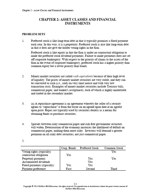
CHAPTER 2: ASSET CLASSES AND FINANCIALINSTRUMENTSPROBLEM SETS1. Preferred stock is like long-term debt in that it typically promises a fixed paymenteach year. In this way, it is a perpetuity. Preferred stock is also like long-term debt in that it does not give the holder voting rights in the firm.Preferred stock is like equity in that the firm is under no contractual obligation tomake the preferred stock dividend payments. Failure to make payments does not set off corporate bankruptcy. With respect to the priority of claims to the assets of thefirm in the event of corporate bankruptcy, preferred stock has a higher priority than common equity but a lower priority than bonds.2. Money market securities are called cash equivalents because of their high levelof liquidity. The prices of money market securities are very stable, and they canbe converted to cash (i.e., sold) on very short notice and with very lowtransaction costs. Examples of money market securities include Treasury bills,commercial paper, and banker's acceptances, each of which is highly marketableand traded in the secondary market.3. (a) A repurchase agreement is an agreement whereby the seller of a securityagrees to “repurchase” it from the buyer on an agreed upon date at an agreedupon price. Repos are typically used by securities dealers as a means forobtaining funds to purchase securities.4. Spreads between risky commercial paper and risk-free government securitieswill widen. Deterioration of the economy increases the likelihood of default oncommercial paper, making them more risky. Investors will demand a greaterpremium on all risky debt securities, not just commercial paper.5.6. Municipal bond interest is tax-exempt at the federal level and possibly at thestate level as well. When facing higher marginal tax rates, a high-incomeinvestor would be more inclined to invest in tax-exempt securities.7. a. You would have to pay the ask price of:161.1875% of par value of $1,000 = $1611.875b. The coupon rate is 6.25% implying coupon payments of $62.50annually or, more precisely, $31.25 semiannually.c. The yield to maturity on a fixed income security is also known as its requiredreturn and is reported by The Wall Street Journal and others in the financialpress as the ask yield. In this case, the yield to maturity is 2.113%. An investorbuying this security today and holding it until it matures will earn an annualreturn of 2.113%. Students will learn in a later chapter how to compute boththe price and the yield to maturity with a financial calculator.8. Treasury bills are discount securities that mature for $10,000. Therefore, a specific T-bill price is simply the maturity value divided by one plus the semi-annual return:P = $10,000/1.02 = $9,803.929. The total before-tax income is $4. After the 70% exclusion for preferred stockdividends, the taxable income is: 0.30 ⨯ $4 = $1.20Therefore, taxes are: 0.30 ⨯ $1.20 = $0.36After-tax income is: $4.00 – $0.36 = $3.64Rate of return is: $3.64/$40.00 = 9.10%10. a. You could buy: $5,000/$64.69 = 77.29 shares. Since it is not possible to tradein fractions of shares, you could buy 77 shares of GD.b. Your annual dividend income would be: 77 ⨯ $2.04 = $157.08c. The price-to-earnings ratio is 9.31 and the price is $64.69. Therefore:$64.69/Earnings per share = 9.3 ⇒ Earnings per share = $6.96d. General Dynamics closed today at $64.69, which was $0.65 higher thanyesterday’s price of $64.0411. a. At t = 0, the value of the index is: (90 + 50 + 100)/3 = 80At t = 1, the value of the index is: (95 + 45 + 110)/3 = 83.333The rate of return is: (83.333/80) - 1 = 4.17%b. In the absence of a split, Stock C would sell for 110, so the value of theindex would be: 250/3 = 83.333 with a divisor of 3.After the split, stock C sells for 55. Therefore, we need to find the divisor(d) such that: 83.333 = (95 + 45 + 55)/d ⇒ d = 2.340. The divisor fell,which is always the case after one of the firms in an index splits its shares.c. The return is zero. The index remains unchanged because the return foreach stock separately equals zero.12. a. Total market value at t = 0 is: ($9,000 + $10,000 + $20,000) = $39,000Total market value at t = 1 is: ($9,500 + $9,000 + $22,000) = $40,500Rate of return = ($40,500/$39,000) – 1 = 3.85%b.The return on each stock is as follows:r A = (95/90) – 1 = 0.0556r B = (45/50) – 1 = –0.10r C = (110/100) – 1 = 0.10The equally weighted average is:[0.0556 + (-0.10) + 0.10]/3 = 0.0185 = 1.85%13. The after-tax yield on the corporate bonds is: 0.09 ⨯ (1 – 0.30) = 0.063 = 6.30%Therefore, municipals must offer a yield to maturity of at least 6.30%.14. Equation (2.2) shows that the equivalent taxable yield is: r = r m/(1 –t), so simplysubstitute each tax rate in the denominator to obtain the following:a. 4.00%b. 4.44%c. 5.00%d. 5.71%15. In an equally weighted index fund, each stock is given equal weight regardless of itsmarket capitalization. Smaller cap stocks will have the same weight as larger cap stocks.The challenges are as follows:•Given equal weights placed to smaller cap and larger cap, equal-weighted indices (EWI) will tend to be more volatile than their market-capitalization counterparts;•It follows that EWIs are not good reflectors of the broad market that they represent; EWIs underplay the economic importance of larger companies.•Turnover rates will tend to be higher, as an EWI must be rebalancedback to its original target. By design, many of the transactions would beamong the smaller, less-liquid stocks.16. a. The ten-year Treasury bond with the higher coupon rate will sell for a higherprice because its bondholder receives higher interest payments.b. The call option with the lower exercise price has more value than one with ahigher exercise price.c. The put option written on the lower priced stock has more value than onewritten on a higher priced stock.17. a. You bought the contract when the futures price was $7.8325 (see Figure2.11 and remember that the number to the right of the apostrophe represents aneighth of a cent). The contract closes at a price of $7.8725, which is $0.04 morethan the original futures price. The contract multiplier is 5000. Therefore, thegain will be: $0.04 ⨯ 5000 = $200.00b. Open interest is 135,778 contracts.18. a. Owning the call option gives you the right, but not the obligation, to buy at$180, while the stock is trading in the secondary market at $193. Since thestock price exceeds the exercise price, you exercise the call.The payoff on the option will be: $193 - $180 = $13The cost was originally $12.58, so the profit is: $13 - $12.58 = $0.42b. Since the stock price is greater than the exercise price, you will exercise the call.The payoff on the option will be: $193 - $185 = $8The option originally cost $9.75, so the profit is $8 - $9.75 = -$1.75c. Owning the put option gives you the right, but not the obligation, to sell at $185,but you could sell in the secondary market for $193, so there is no value inexercising the option. Since the stock price is greater than the exercise price,you will not exercise the put. The loss on the put will be the initial cost of$12.01.19. There is always a possibility that the option will be in-the-money at some time prior toexpiration. Investors will pay something for this possibility of a positive payoff.20.Value of Call at Expiration Initial Cost Profita. 0 4 -4b. 0 4 -4c. 0 4 -4d. 5 4 1e. 10 4 6Value of Put at Expiration Initial Cost Profita. 10 6 4b. 5 6 -1c. 0 6 -6d. 0 6 -6e. 0 6 -621. A put option conveys the right to sell the underlying asset at the exercise price. Ashort position in a futures contract carries an obligation to sell the underlying assetat the futures price. Both positions, however, benefit if the price of the underlyingasset falls.22. A call option conveys the right to buy the underlying asset at the exercise price. Along position in a futures contract carries an obligation to buy the underlying assetat the futures price. Both positions, however, benefit if the price of the underlyingasset rises.CFA PROBLEMS1.(d) There are tax advantages for corporations that own preferred shares.2. The equivalent taxable yield is: 6.75%/(1 0.34) = 10.23%3. (a) Writing a call entails unlimited potential losses as the stock price rises.4. a. The taxable bond. With a zero tax bracket, the after-tax yield for thetaxable bond is the same as the before-tax yield (5%), which is greater thanthe yield on the municipal bond.b. The taxable bond. The after-tax yield for the taxable bond is:0.05⨯ (1 – 0.10) = 4.5%c. You are indifferent. The after-tax yield for the taxable bond is:0.05 ⨯ (1 – 0.20) = 4.0%The after-tax yield is the same as that of the municipal bond.d. The municipal bond offers the higher after-tax yield for investors in taxbrackets above 20%.5.If the after-tax yields are equal, then: 0.056 = 0.08 × (1 –t)This implies that t = 0.30 =30%.。
投资学(博迪)第10版课后习题答...
投资学(博迪)第10版课后习题答...CHAPTER 10: ARBITRAGE PRICING THEORY ANDMULTIFACTOR MODELS OF RISK AND RETURN PROBLEM SETS1. The revised estimate of the expected rate of return on the stock would be the oldestimate plus the sum of the products of the unexpected change in each factor times the respective sensitivity coefficient: Revised estimate = 12% + [(1 × 2%) + (0.5 × 3%)] = 15.5%Note that the IP estimate is computed as: 1 × (5% - 3%), and the IR estimate iscomputed as: 0.5 × (8% - 5%).2. The APT factors must correlate with major sources of uncertainty, i.e., sources ofuncertainty that are of concern to many investors. Researchers should investigatefactors that correlate with uncertainty in consumption and investment opportunities.GDP, the inflation rate, and interest rates are among the factors that can be expected to determine risk premiums. In particular, industrial production (IP) is a goodindicator of changes in the business cycle. Thus, IP is a candidate for a factor that is highly correlated with uncertainties that have to do with investment andconsumption opportunities in the economy.3. Any pattern of returns can be explained if we are free to choose an indefinitelylarge number of explanatory factors. If a theory of asset pricing is to have value, itmust explain returns using a reasonably limited number of explanatory variables(i.e., systematic factors such as unemployment levels, GDP, and oil prices).4. Equation 10.11 applies here:E(r p) = r f + βP1 [E(r1 ) ?r f ] + βP2 [E(r2 ) – r f]We need to find the risk premium (RP) for each of the two factors:RP1 = [E(r1 ) ?r f] and RP2 = [E(r2 ) ?r f]In order to do so, we solve the following system of two equations with two unknowns: .31 = .06 + (1.5 ×RP1 ) + (2.0 ×RP2 ).27 = .06 + (2.2 ×RP1 ) + [(–0.2) ×RP2 ]The solution to this set of equations isRP1 = 10% and RP2 = 5%Thus, the expected return-beta relationship isE(r P) = 6% + (βP1× 10%) + (βP2× 5%)5. The expected return for portfolio F equals the risk-free rate since its beta equals 0.For portfolio A, the ratio of risk premium to beta is (12 ?6)/1.2 = 5For portfolio E, the ratio is lower at (8 – 6)/0.6 = 3.33This implies that an arbitrage opportunity exists. For instance, you can create aportfolio G with beta equal to 0.6 (the same as E’s) by combining portfolio A and portfolio F in equal weights. The expected return and beta for portfolio G are then: E(r G) = (0.5 × 12%) + (0.5 × 6%) = 9%βG = (0.5 × 1.2) + (0.5 × 0%) = 0.6Comparing portfolio G to portfolio E, G has the same betaand higher return.Therefore, an arbitrage opportunity exists by buying portfolio G and selling anequal amount of portfolio E. The profit for this arbitrage will ber G –r E =[9% + (0.6 ×F)] ?[8% + (0.6 ×F)] = 1%That is, 1% of the funds (long or short) in each portfolio.6. Substituting the portfolio returns and betas in the expected return-beta relationship,we obtain two equations with two unknowns, the risk-free rate (r f) and the factor risk premium (RP):12% = r f + (1.2 ×RP)9% = r f + (0.8 ×RP)Solving these equations, we obtainr f = 3% and RP = 7.5%7. a. Shorting an equally weighted portfolio of the ten negative-alpha stocks andinvesting the proceeds in an equally-weighted portfolio of the 10 positive-alpha stocks eliminates the market exposure and creates a zero-investmentportfolio. Denoting the systematic market factor as R M, the expected dollarreturn is (noting that the expectation of nonsystematic risk, e, is zero):$1,000,000 × [0.02 + (1.0 ×R M)] ? $1,000,000 × [(–0.02) + (1.0 ×R M)]= $1,000,000 × 0.04 = $40,000The sensitivity of the payoff of this portfolio to the market factor is zerobecause the exposures of the positive alpha and negative alpha stocks cancelout. (Notice that the terms involving R M sum to zero.) Thus, the systematiccomponent of total risk is also zero. The variance of the analyst’s profit is notzero, however, since this portfolio is not well diversified.For n = 20 stocks (i.e., long 10 stocks and short 10 stocks) the investor willhave a $100,000 position (either long or short) in each stock. Net marketexposure is zero, but firm-specific risk has not been fully diversified. Thevariance of dollar returns from the positions in the 20 stocks is20 × [(100,000 × 0.30)2] = 18,000,000,000The standard deviation of dollar returns is $134,164.b. If n = 50 stocks (25 stocks long and 25 stocks short), the investor will have a$40,000 position in each stock, and the variance of dollar returns is50 × [(40,000 × 0.30)2] = 7,200,000,000The standard deviation of dollar returns is $84,853.Similarly, if n = 100 stocks (50 stocks long and 50 stocks short), the investorwill have a $20,000 position in each stock, and the variance of dollar returns is100 × [(20,000 × 0.30)2] = 3,600,000,000The standard deviation of dollar returns is $60,000.Notice that, when the number of stocks increases by a factorof 5 (i.e., from 20 to 100), standard deviation decreases by a factor of 5= 2.23607 (from$134,164 to $60,000).8. a. )(σσβσ2222e M +=88125)208.0(σ2222=+×=A50010)200.1(σ2222=+×=B97620)202.1(σ2222=+×=Cb. If there are an infinite number of assets with identical characteristics, then awell-diversified portfolio of each type will have only systematic risk since thenonsystematic risk will approach zero with large n. Each variance is simply β2 × market variance:222Well-diversified σ256Well-diversified σ400Well-diversified σ576A B C;;;The mean will equal that of the individual (identical) stocks.c. There is no arbitrage opportunity because the well-diversified portfolios allplot on the security market line (SML). Because they are fairly priced, there isno arbitrage.9. a. A long position in a portfolio (P) composed of portfoliosA andB will offer anexpected return-beta trade-off lying on a straight linebetween points A and B.Therefore, we can choose weights such that βP = βC but with expected returnhigher than that of portfolio C. Hence, combining P with a short position in Cwill create an arbitrage portfolio with zero investment, zero beta, and positiverate of return.b. The argument in part (a) leads to the proposition that the coefficient of β2must be zero in order to preclude arbitrage opportunities.10. a. E(r) = 6% + (1.2 × 6%) + (0.5 × 8%) + (0.3 × 3%) = 18.1%b.Surprises in the macroeconomic factors will result in surprises in the return ofthe stock:Unexpected return from macro factors =[1.2 × (4% –5%)] + [0.5 × (6% –3%)] + [0.3 × (0% – 2%)] = –0.3%E(r) =18.1% ? 0.3% = 17.8%11. The APT required (i.e., equilibrium) rate of return on the stock based on r f and thefactor betas isRequired E(r) = 6% + (1 × 6%) + (0.5 × 2%) + (0.75 × 4%) = 16% According to the equation for the return on the stock, the actually expected return on the stock is 15% (because the expected surprises on all factors are zero bydefinition). Because the actually expected return based on risk is less than theequilibrium return, we conclude that the stock is overpriced.12. The first two factors seem promising with respect to thelikely impact on the firm’scost of capital. Both are macro factors that would elicit hedging demands acrossbroad sectors of investors. The third factor, while important to Pork Products, is a poor choice for a multifactor SML because the price of hogs is of minor importance to most investors and is therefore highly unlikely to be a priced risk factor. Better choices would focus on variables that investors in aggregate might find moreimportant to their welfare. Examples include: inflation uncertainty, short-terminterest-rate risk, energy price risk, or exchange rate risk. The important point here is that, in specifying a multifactor SML, we not confuse risk factors that are important toa particular investor with factors that are important to investors in general; only the latter are likely to command a risk premium in the capital markets.13. The formula is ()0.04 1.250.08 1.50.02.1717%E r =+×+×==14. If 4%f r = and based on the sensitivities to real GDP (0.75) and inflation (1.25),McCracken would calculate the expected return for the Orb Large Cap Fund to be:()0.040.750.08 1.250.02.040.0858.5% above the risk free rate E r =+×+×=+=Therefore, Kwon’s fundamental analysis estimate is congruent with McCr acken’sAPT estimate. If we assume that both Kwon and McCracken’s estimates on the return of Orb’s Large Cap Fund are accurate, then no arbitrage profit is possible.15. In order to eliminate inflation, the following three equations must be solvedsimultaneously, where the GDP sensitivity will equal 1 in the first equation,inflation sensitivity will equal 0 in the second equation and the sum of the weights must equal 1 in the third equation.1.1.250.75 1.012.1.5 1.25 2.003.1wx wy wz wz wy wz wx wy wz ++=++=++=Here, x represents Orb’s High Growth Fund, y represents Large Cap Fund and z represents Utility Fund. Using algebraic manipulation will yield wx = wy = 1.6 and wz = -2.2.16. Since retirees living off a steady income would be hurt by inflation, this portfoliowould not be appropriate for them. Retirees would want a portfolio with a return positively correlated with inflation to preserve value, and less correlated with the variable growth of GDP. Thus, Stiles is wrong. McCracken is correct in that supply side macroeconomic policies are generally designed to increase output at aminimum of inflationary pressure. Increased output would mean higher GDP, which in turn would increase returns of a fund positively correlated with GDP.17. The maximum residual variance is tied to the number of securities (n ) in theportfolio because, as we increase the number of securities, we are more likely to encounter securities with larger residual variances. The starting point is todetermine the practical limit on the portfolio residualstandard deviation, σ(e P ), that still qualifies as a well-diversified portfolio. A reasonable approach is to compareσ2(e P) to the market variance, or equivalently, to compare σ(e P) to the market standard deviation. Suppose we do n ot allow σ(e P) to exceed pσM, where p is a small decimal fraction, for example, 0.05; then, the smaller the value we choose for p, the more stringent our criterion for defining how diversified a well-diversified portfolio must be.Now construct a portfolio of n securities with weights w1, w2,…,w n, so that Σw i =1. The portfolio residual variance is σ2(e P) = Σw12σ2(e i)To meet our practical definition of sufficiently diversified, we require this residual variance to be less than (pσM)2. A sure and simple way to proceed is to assume the worst, that is, assume that the residual variance of each security is the highest possible value allowed under the assumptions of the problem: σ2(e i) = nσ2MIn that case σ2(e P) = Σw i2 nσM2Now apply the constraint: Σw i2nσM2 ≤ (pσM)2This requires that: nΣw i2 ≤ p2Or, equivalently, that: Σw i2 ≤ p2/nA relatively easy way to generate a set of well-diversified portfolios is to use portfolio weights that follow a geometric progression, since the computations then become relatively straightforward. Choose w1 and a common factor q for the geometric progression such that q < 1. Therefore, the weight on each stock is a fraction q of the weight on the previous stock in the series. Then the sum of n terms is:Σw i= w1(1– q n)/(1– q) = 1or: w1 = (1– q)/(1– q n)The sum of the n squared weights is similarly obtained from w12 and a common geometric progression factor of q2. ThereforeΣw i2 = w12(1– q2n)/(1– q 2)Substituting for w1 from above, we obtainΣw i2 = [(1– q)2/(1– q n)2] × [(1– q2n)/(1– q 2)]For sufficient diversification, we choose q so that Σw i2 ≤ p2/nFor example, continue to assume that p = 0.05 and n = 1,000. If we chooseq = 0.9973, then we will satisfy the required condition. At this value for q w1 = 0.0029 and w n = 0.0029 × 0.99731,000 In this case, w1 is about 15 times w n. Despite this significant departure from equal weighting, this portfolio is nevertheless well diversified. Any value of q between0.9973 and 1.0 results in a well-diversified portfolio. As q gets closer to 1, theportfolio approaches equal weighting.18. a. Assume a single-factor economy, with a factor risk premium E M and a (large)set of well-diversified portfolios with beta βP. Suppose we create a portfolio Zby allocating the portion w to portfolio P and (1 – w) to the market portfolioM. The rate of return on portfolio Z is:R Z = (w × R P) + [(1 –w) × R M]Portfolio Z is riskless if we choose w so that βZ = 0. This requires that:βZ = (w × βP) + [(1 –w) × 1] = 0 ?w = 1/(1 –βP) and (1 – w) = –βP/(1 –βP)Substitute this value for w in the expression for R Z:R Z = {[1/(1 –βP)] × R P} –{[βP/(1 –βP)] × R M}Since βZ = 0, then, in order to avoid arbitrage, R Z must be zero.This implies that: R P = βP × R MTaking expectations we have:E P = βP × E MThis is the SML for well-diversified portfolios.b. The same argument can be used to show that, in a three-factor model withfactor risk premiums E M, E1 and E2, in order to avoid arbitrage, we must have:E P = (βPM × E M) + (βP1 × E1) + (βP2 × E2)This is the SML for a three-factor economy.19. a. The Fama-French (FF) three-factor model holds that one of the factors drivingreturns is firm size. An index with returns highly correlated with firm size (i.e.,firm capitalization) that captures this factor is SMB (small minus big), thereturn for a portfolio of small stocks in excess of the return for a portfolio oflarge stocks. The returns for a small firm will be positively correlated withSMB. Moreover, the smaller the firm, the greater its residual from the othertwo factors, the market portfolio and the HML portfolio, which is the returnfor a portfolio of high book-to-market stocks in excess of the return for aportfolio of low book-to-market stocks. Hence, the ratio of the variance of thisresidual to the variance of the return on SMB will be larger and, together withthe higher correlation, results in a high beta on the SMB factor.b.This question appears to point to a flaw in the FF model. The model predictsthat firm size affects average returns so that, if two firms merge into a largerfirm, then the FF model predicts lower average returns for the merged firm.However, there seems to be no reason for the merged firm to underperformthe returns of the component companies, assuming that the component firmswere unrelated and that they will now be operated independently. We mighttherefore expect that the performance of the merged firm would be the sameas the performance of a portfolio of the originally independent firms, but theFF model predicts that the increased firm size will result in lower averagereturns. Therefore, the question revolves around the behavior of returns for aportfolio of small firms, compared to the return for larger firms that resultfrom merging those small firms into larger ones. Had past mergers of smallfirms into larger firms resulted, on average, in no change in the resultantlarger firms’ stock return characteristics (compared to the portfolio of stocksof the merged firms), the size factor in the FF model would have failed.Perhaps the reason the size factor seems to help explain stock returns is that,when small firms become large, the characteristics of their fortunes (andhence their stock returns) change in a significant way. Put differently, stocksof large firms that result from a merger of smaller firms appear empirically tobehave differently from portfolios of the smaller component firms.Specifically, the FF model predicts that the large firm will have a smaller riskpremium. Notice that this development is not necessarily a bad thing for thestockholders of the smaller firms that merge. The lower risk premium may bedue, in part, to the increase in value of the larger firm relative to the mergedfirms.CFA PROBLEMS1. a. This statement is incorrect. The CAPM requires a mean-variance efficientmarket portfolio, but APT does not.b.This statement is incorrect. The CAPM assumes normallydistributed securityreturns, but APT does not.c. This statement is correct.2. b. Since portfolio X has β = 1.0, then X is the market portfolio and E(R M) =16%.Using E(R M ) = 16% and r f = 8%, the expected return for portfolio Y is notconsistent.3. d.4. c.5. d.6. c. Investors will take on as large a position as possible only if the mispricingopportunity is an arbitrage. Otherwise, considerations of risk anddiversification will limit the position they attempt to take in the mispricedsecurity.7. d.8. d.。
博迪《投资学》笔记和课后习题详解(资产组合业绩评估)【圣才出品】

第24章资产组合业绩评估24.1 复习笔记1.测算投资收益(1)时间加权收益率与货币加权收益率内部收益率,又称为投资的货币加权收益率。
之所以称它是货币加权的,是因为在测算该收益率时,不同时期的持股数对平均收益率有更大的影响。
时间加权收益率忽略了不同时期所持股数的不同,只考虑了每一期的收益,而忽略了每一期股票投资额之间的不同。
一般来说,货币加权和时间加权的收益率是不同的,孰高孰低取决于收益的时间结构和资产组合的成分。
对于单个投资者来说,货币加权收益率应该更准确些;但对于资金管理行业来说,由于投资额度的不确定性通常采用时间加权收益率来评估其业绩。
(2)算术平均与几何平均时间加权收益率与货币加权收益率两种方法为算术平均收益率,另一种方法为几何平均收益率。
一般情况下,对于一个n期投资来说,其几何平均收益率如下:其中,r t(t=1,2,…,n)为每期的收益率。
几何平均收益率绝不会超过算术平均收益率,而且在几何平均收益率的算法中,较低的收益率具有更大的影响,得出几何平均收益率要比算术平均收益率低一些。
算术平均收益率是预期未来业绩的正确方法。
2.业绩评估的传统理论(1)合适的业绩评估指标①夏普测度:夏普测度是用资产组合的长期平均超额收益除以这个时期收益的标准差。
它测度了对总波动性权衡的回报,适用于该资产组合就是投资者所有投资的情况。
②特雷纳测度:与夏普测度指标相类似,特雷纳测度给出了单位风险的超额收益,但它用的是系统风险而不是全部风险。
其适用于该资产组合只是众多子资产组合中某个资产组合的情况。
③詹森测度(组合阿尔法值):詹森测度是建立在CAPM测算基础上的资产组合的平均收益,它用到了资产组合的贝塔值和平均市场收益,其结果即为资产组合的阿尔法值。
其适用范围同特雷纳测度一致。
④信息比率(也称估价比率):信息比率这种方法用资产组合的阿尔法值除以其非系统风险,它测算的是每单位非系统风险所带来的非常规收益,前者是指在原则上可以通过持有市场上全部资产组合而完全分散掉的那一部分风险。
博迪《投资学》(第10版)笔记和课后习题详解答案

博迪《投资学》(第10版)笔记和课后习题详解答案博迪《投资学》(第10版)笔记和课后习题详解完整版>精研学习?>无偿试用20%资料全国547所院校视频及题库全收集考研全套>视频资料>课后答案>往年真题>职称考试第一部分绪论第1章投资环境1.1复习笔记1.2课后习题详解第2章资产类别与金融工具2.1复习笔记2.2课后习题详解第3章证券是如何交易的3.1复习笔记3.2课后习题详解第4章共同基金与其他投资公司4.1复习笔记4.2课后习题详解第二部分资产组合理论与实践第5章风险与收益入门及历史回顾5.1复习笔记5.2课后习题详解第6章风险资产配置6.1复习笔记6.2课后习题详解第7章最优风险资产组合7.1复习笔记7.2课后习题详解第8章指数模型8.2课后习题详解第三部分资本市场均衡第9章资本资产定价模型9.1复习笔记9.2课后习题详解第10章套利定价理论与风险收益多因素模型10.1复习笔记10.2课后习题详解第11章有效市场假说11.1复习笔记11.2课后习题详解第12章行为金融与技术分析12.1复习笔记12.2课后习题详解第13章证券收益的实证证据13.1复习笔记13.2课后习题详解第四部分固定收益证券第14章债券的价格与收益14.1复习笔记14.2课后习题详解第15章利率的期限结构15.1复习笔记15.2课后习题详解第16章债券资产组合管理16.1复习笔记16.2课后习题详解第五部分证券分析第17章宏观经济分析与行业分析17.2课后习题详解第18章权益估值模型18.1复习笔记18.2课后习题详解第19章财务报表分析19.1复习笔记19.2课后习题详解第六部分期权、期货与其他衍生证券第20章期权市场介绍20.1复习笔记20.2课后习题详解第21章期权定价21.1复习笔记21.2课后习题详解第22章期货市场22.1复习笔记22.2课后习题详解第23章期货、互换与风险管理23.1复习笔记23.2课后习题详解第七部分应用投资组合管理第24章投资组合业绩评价24.1复习笔记24.2课后习题详解第25章投资的国际分散化25.1复习笔记25.2课后习题详解第26章对冲基金26.1复习笔记26.2课后习题详解第27章积极型投资组合管理理论27.1复习笔记27.2课后习题详解第28章投资政策与特许金融分析师协会结构28.1复习笔记28.2课后习题详解。
博迪《投资学》(第10版)章节题库-第九章至第十章【圣才出品】
第三部分资本市场均衡第9章资本资产定价模型一、选择题1.如果一个股票的价值是高估的,则它应位于()。
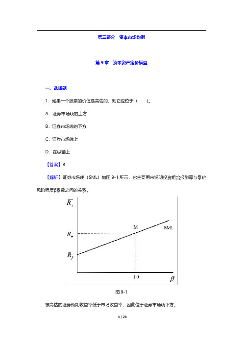
A.证券市场线的上方B.证券市场线的下方C.证券市场线上D.在纵轴上【答案】B【解析】证券市场线(SML)如图9-1所示,它主要用来说明投资组合报酬率与系统风险程度β系数之间的关系。
图9-1被高估的证券预期收益率低于市场收益率,因此位于证券市场线下方。
2.无风险利率和市场预期收益率分别是3.5%和10.5%。
根据资本资产定价模型,一只β值是1.63的证券的预期收益是()。
A.10.12%B.14.91%C.16.56%D.18.79%【答案】B【解析】根据资本资产定价模型:E(r i)=r f+β[E(r M)-r f]=3.5%+1.63×(10.5%-3.5%)=14.91%。
3.资本资产定价模型给出了精确预测()的方法。
A.有效投资组合B.单一资产与风险资产组合期望收益率C.不同风险收益偏好下最优风险投资组合D.资产风险及其期望收益率之间的关系【答案】D【解析】根据资本资产定价模型,每一证券的期望收益率应等于无风险利率加上该证券由β系数测定的风险溢价。
4.假定一只股票定价合理,预期收益是15%,市场预期收益是10.5%,无风险利率是3.5%,这只股票的β值是()。
A.1.36B.1.52C.1.64D.1.75【答案】C【解析】既然α值假定为零,证券的收益就等于CAPM设定的收益。
因此,将已知的数值代入CAPM,即15%=[3.5%+(10.5%-3.5%)β],解得:β=1.64。
5.根据CAPM模型,市场期望收益率和无风险收益率分别是0.12和0.06,β值为1.2的证券A的期望收益率是()。
A.0.068B.0.12C.0.132D.0.142【答案】C【解析】根据资本资产定价模型,E(r i)=r f+[E(r M)-r f]βi=0.06+(0.12-0.06)×1.2=0.132。
博迪《投资学》笔记和课后习题详解(最优风险资产组合)【圣才出品】

第8章最优风险资产组合8.1 复习笔记1. 分散化与资产组合风险(1)系统性风险与非系统性风险分散化能够降低风险,但是当共同的风险来源影响所有的公司时,分散化就不能消除风险了。
资产组合的标准差随着证券种类的增加而下降,但是,它不能降至零。
在最充分的分散条件下还存在着市场风险,它来源于与市场有关的因素,这种风险亦被称为“系统风险”,或“不可分散风险”。
而那些可被分散化消除的风险被称为“独特风险”、“特有公司风险”、“非系统风险”或“可分散风险”。
(2)两种风险资产的资产组合①资产组合的风险与收益资产组合的期望收益是资产组合中各种证券的期望收益的加权平均值,即:两资产的资产组合的方差是:②表格法计算组合方差表8-1显示可以通过电子表格计算资产组合的方差。
其中a表示两个共同基金收益的相邻协方差矩阵,相邻矩阵是沿着首排首列相邻每一基金在资产组合中权重的协方差矩阵。
可以通过如下方法得到资产组合的方差:斜方差矩阵中的每个因子与行、列中的权重相乘,把四个结果相加,就可以得出给出的资产组合方差。
表8-1 通过协方差矩阵计算资产组合方差③相关系数与资产组合方差具有完全正相关(相关系数为1)的资产组合的标准差恰好是资产组合中各证券标准差的加权平均值。
相关系数小于1时,资产组合的标准差小于资产组合中各证券标准差的加权平均值。
通过调整资产比例,具有完全负相关(相关系数为-1)的资产组合的标准差可以趋向0。
④资产组合比例与资产组合方差当两种资产负相关时,调整资产组合比例可以得到小于两种资产方差的最小组合方差。
若某个资产比例为负值,表示借入(或卖空)该资产。
⑤机会集机会集是指多种资产进行组合所能构成的所有风险收益的集合。
2. 资产配置(1)最优风险资产组合最优风险资产组合是使资本配置线的斜率(报酬与波动比率)最大的风险资产组合,这样表示边际风险报酬最大。
最优风险资产组合为资产配置线与机会集曲线的切点。
(2)最优完整资产组合最优完整资产组合为投资者无差异曲线与资本配置线的切点处组合,最优完整组合包含风险资产组合(债券和股票)以及无风险资产(国库券)。
投资学第10版课后习题答案
CHAPTER 4: MUTUAL FUNDS AND OTHER INVESTMENTCOMPANIESPROBLEM SETS1. The unit investment trust should have lower operating expenses.Because the investment trust portfolio is fixed once the trust isestablished, it does not have to pay portfolio managers toconstantly monitor and rebalance the portfolio as perceived needsor opportunities change. Because the portfolio is fixed, the unitinvestment trust also incurs virtually no trading costs.2. a. Unit investment trusts: Diversification from large-scaleinvesting, lower transaction costs associated with large-scaletrading, low management fees, predictable portfolio composition,guaranteed low portfolio turnover rate.b. Open-end mutual funds: Diversification from large-scaleinvesting, lower transaction costs associated with large-scaletrading, professional management that may be able to takeadvantage of buy or sell opportunities as they arise, recordkeeping.c. Individual stocks and bonds: No management fee; ability tocoordinate realization of capital gains or losses withinvestors’ personal tax situation s; capability of designingportfolio to investor’s specific risk and return profile.3. Open-end funds are obligated to redeem investor's shares at netasset value and thus must keep cash or cash-equivalent securitieson hand in order to meet potential redemptions. Closed-end funds do not need the cash reserves because there are no redemptions forclosed-end funds. Investors in closed-end funds sell their shareswhen they wish to cash out.4. Balanced funds keep relatively stable proportions of funds investedin each asset class. They are meant as convenient instruments toprovide participation in a range of asset classes. Life-cycle fundsare balanced funds whose asset mix generally depends on the age of the investor. Aggressive life-cycle funds, with larger investments in equities, are marketed to younger investors, while conservative life-cycle funds, with larger investments in fixed-income securities, are designed for older investors. Asset allocation funds, in contrast, may vary the proportions invested in each asset class by large amounts as predictions of relative performance across classes vary. Asset allocation funds therefore engage in more aggressive market timing.5. Unlike an open-end fund, in which underlying shares are redeemedwhen the fund is redeemed, a closed-end fund trades as a security in the market. Thus, their prices may differ from the NAV.6. Advantages of an ETF over a mutual fund:ETFs are continuously traded and can be sold or purchased on margin.There are no capital gains tax triggers when an ETF is sold(shares are just sold from one investor to another).Investors buy from brokers, thus eliminating the cost ofdirect marketing to individual small investors. This implieslower management fees.Disadvantages of an ETF over a mutual fund:Prices can depart from NAV (unlike an open-end fund).There is a broker fee when buying and selling (unlike a no-load fund).7. The offering price includes a 6% front-end load, or salescommission, meaning that every dollar paid results in only $ going toward purchase of shares. Therefore: Offering price =06.0170.10$Load 1NAV -=-= $8. NAV = Offering price (1 –Load) = $ .95 = $9. Stock Value Held by FundA $ 7,000,000B 12,000,000C 8,000,000D 15,000,000Total $42,000,000Net asset value =000,000,4000,30$000,000,42$-= $10. Value of stocks sold and replaced = $15,000,000 Turnover rate =000,000,42$000,000,15$= , or %11. a. 40.39$000,000,5000,000,3$000,000,200$NAV =-=b. Premium (or discount) = NAVNAV ice Pr - = 40.39$40.39$36$-= –, or % The fund sells at an % discount from NAV.12. 100NAV NAV Distributions $12.10$12.50$1.500.088, or 8.8%NAV $12.50-+-+==13. a. Start-of-year price: P 0 = $ × = $End-of-year price: P 1 = $ × = $Although NAV increased by $, the price of the fund decreased by $. Rate of return =100Distributions $11.25$12.24$1.500.042, or 4.2%$12.24P P P -+-+==b. An investor holding the same securities as the fund managerwould have earned a rate of return based on the increase in the NAV of the portfolio:100NAV NAV Distributions $12.10$12.00$1.500.133, or 13.3%NAV $12.00-+-+==14. a. Empirical research indicates that past performance of mutualfunds is not highly predictive of future performance,especially for better-performing funds. While there may be some tendency for the fund to be an above average performer nextyear, it is unlikely to once again be a top 10% performer.b. On the other hand, the evidence is more suggestive of atendency for poor performance to persist. This tendency isprobably related to fund costs and turnover rates. Thus if the fund is among the poorest performers, investors should beconcerned that the poor performance will persist.15. NAV 0 = $200,000,000/10,000,000 = $20Dividends per share = $2,000,000/10,000,000 = $NAV1 is based on the 8% price gain, less the 1% 12b-1 fee: NAV1 = $20 (1 – = $Rate of return =20$20 .0$20$384.21$+-= , or %16. The excess of purchases over sales must be due to new inflows intothe fund. Therefore, $400 million of stock previously held by the fund was replaced by new holdings. So turnover is: $400/$2,200 = , or %.17. Fees paid to investment managers were: $ billion = $ millionSince the total expense ratio was % and the management fee was %, we conclude that % must be for other expenses. Therefore, other administrative expenses were: $ billion = $ million.18. As an initial approximation, your return equals the return on the shares minus the total of the expense ratio and purchase costs: 12% % 4% = %.But the precise return is less than this because the 4% load is paid up front, not at the end of the year. To purchase the shares, you would have had to invest: $20,000/(1 = $20,833. The shares increase in value from $20,000 to: $20,000 = $22,160. The rate of return is: ($22,160 $20,833)/$20,833 = %.19. Assume $1,000 investmentLoaded-Up Fund Economy Fund Yearly growth (r is 6%) (1.01.0075)r +-- (.98)(1.0025)r ⨯+- t = 1 year$1, $1, t = 3 years$1, $1, t = 10 years$1, $1,20. a. $450,000,000$10,000000$1044,000,000-= b. The redemption of 1 million shares will most likely triggercapital gains taxes which will lower the remaining portfolio by an amount greater than $10,000,000 (implying a remaining total value less than $440,000,000). The outstanding shares fall to 43 million and the NAV drops to below $10.21. Suppose you have $1,000 to invest. The initial investment in ClassA shares is $940 net of the front-end load. After four years, yourportfolio will be worth:$940 4 = $1,Class B shares allow you to invest the full $1,000, but yourinvestment performance net of 12b-1 fees will be only %, and you will pay a 1% back-end load fee if you sell after four years. Your portfolio value after four years will be:$1,000 4 = $1,After paying the back-end load fee, your portfolio value will be:$1, .99 = $1,Class B shares are the better choice if your horizon is four years.With a 15-year horizon, the Class A shares will be worth:$940 15 = $3,For the Class B shares, there is no back-end load in this casesince the horizon is greater than five years. Therefore, the value of the Class B shares will be:$1,000 15 = $3,At this longer horizon, Class B shares are no longer the betterchoice. The effect of Class B's % 12b-1 fees accumulates over time and finally overwhelms the 6% load charged to Class A investors.22. a. After two years, each dollar invested in a fund with a 4% loadand a portfolio return equal to r will grow to: $ (1 + r–2.Each dollar invested in the bank CD will grow to: $1 .If the mutual fund is to be the better investment, then theportfolio return (r) must satisfy:(1 + r–2 >(1 + r–2 >(1 + r–2 >1 + r– >1 + r >Therefore: r > = %b. If you invest for six years, then the portfolio return mustsatisfy:(1 + r–6 > =(1 + r–6 >1 + r– >r > %The cutoff rate of return is lower for the six-year investment because the “fixed cost” (the one-time front-end load) is spread over a greater number of years.c. With a 12b-1 fee instead of a front-end load, the portfoliomust earn a rate of return (r ) that satisfies:1 + r – – >In this case, r must exceed % regardless of the investmenthorizon.23. The turnover rate is 50%. This means that, on average, 50% of theportfolio is sold and replaced with other securities each year. Trading costs on the sell orders are % and the buy orders toreplace those securities entail another % in trading costs. Total trading costs will reduce portfolio returns by: 2 % = %24. For the bond fund, the fraction of portfolio income given up tofees is: %0.4%6.0= , or % For the equity fund, the fraction of investment earnings given up to fees is:%0.12%6.0= , or % Fees are a much higher fraction of expected earnings for the bond fund and therefore may be a more important factor in selecting the bond fund.This may help to explain why unmanaged unit investment trusts are concentrated in the fixed income market. The advantages of unit investment trusts are low turnover, low trading costs, and low management fees. This is a more important concern to bond-market investors.25. Suppose that finishing in the top half of all portfolio managers ispurely luck, and that the probability of doing so in any year is exactly ½. Then the probability that any particular manager would finish in the top half of the sample five years in a row is (½)5 = 1/32. We would then expect to find that [350 (1/32)] = 11managers finish in the top half for each of the five consecutiveyears. This is precisely what we found. Thus, we should not conclude that the consistent performance after five years is proof of skill. We would expect to find 11 managers exhibiting precisely this level of "consistency" even if performance is due solely to luck.。
- 1、下载文档前请自行甄别文档内容的完整性,平台不提供额外的编辑、内容补充、找答案等附加服务。
- 2、"仅部分预览"的文档,不可在线预览部分如存在完整性等问题,可反馈申请退款(可完整预览的文档不适用该条件!)。
- 3、如文档侵犯您的权益,请联系客服反馈,我们会尽快为您处理(人工客服工作时间:9:00-18:30)。
第二部分资产组合理论与实践
第5章风险与收益入门及历史回顾
5.1复习笔记
1.利率水平的决定因素
(1)预测利率的基本因素
利率水平及其未来利率的预测是投资决策中非常重要的部分。
预测利率首先基于以下一些基本因素:
①存款人(主要是家庭)的资金供给。
②企业由于购置厂房设备及存货而进行项目融资所引发的资金需求。
③政府通过美联储运作产生的资金净供给或净需求。
(2)实际利率与名义利率
名义利率是资金量增长率,实际利率是购买力增长率,设名义利率为R,实际利率为r,通胀率为i,则有下式近似成立r≈R-i,换句话说,实际利率等于名义利率减去通胀率。
严格上讲,名义利率和实际利率之间有下式成立:
1+r=(1+R)/(1+i)
购买力增长值(1+r)等于货币增长值(1+R)除以新的价格水平(1+i),由上式推导得到:
r=(R-i)/(1+i)
显然可以看出由r≈R-i得出的近似值高估了实际利率1+i倍。
(3)均衡实际利率与名义利率
①均衡实际利率
实际利率由三个基本因素决定:供给、需求和政府行为。
图5-1描绘了一条向下倾斜的需求曲线和一条向上倾斜的供给曲线,横轴代表资金的数量,纵轴代表实际利率。
供给曲线向上倾斜是因为实际利率越高,居民储蓄的需求也就越大。
这个假设基于这样的原理:实际利率高,居民会推迟现时消费转为未来消费并进行现时投资。
需求曲线向下倾斜是因为实际利率偏低,厂商会加大其资本投资的力度。
供给曲线与需求曲线的交点形成图5-1中的均衡点E。
政府和中央银行(美联储)可以通过财政政策或者货币政策向左或向右移动供给曲线和需求曲线。
例如,假定政府预算赤字增加,政府需要增加借款,推动需求曲线向右平移,均衡点从E点移至E′点。
图5-1均衡实际利率的决定
②均衡名义利率
资产的实际收益率等于名义利率减去通胀率,因此,当通胀率增加时,投资者会对其投资提出更高的名义利率要求,从而保证投资项目所提供的实际利率不变。
欧文·费雪认为名义利率应当伴随着预期通胀率的增加而增加。
假设目前的预期通胀率
将持续到下一时期,记为E(i),那么费雪等式为:R=r+E(i),这表明如果实际利率是稳定的,名义利率的上涨意味着更高的通胀率。
实证研究很难证实费雪关于名义利率的上涨意味着有一更高的通胀率的假设,这是因为往往实际利率也在发生着无法预测的变化。
名义利率可以被视为是名义上无风险资产的必要收益率加上通胀的预测值。
(4)税收与实际利率
假设税率为t,名义利率为R,则税后名义利率为R(1-t)。
税后实际利率近似等于税后名义利率减去通货膨胀率,即:
R(1-t)-i=(r+i)(1-t)-i=r(1-t)-it
因此,税后实际利率随着通货膨胀率的上升而下降,投资者承受了相当于税率乘以通货膨胀率的损失。
2.比较不同持有期的收益率
(1)有效年利率
在比较不同持有期的投资收益时,可以将每一个总收益换算成某一常用期限的收益率。
我们通常把一年内所有的投资收益表达为有效年利率(EAR),即一年期投资价值增长百分比。
对于一年期的投资来说,有效年利率等于总收益率r f(1),总收入(1+EAR)是每一美元投资的最终价值。
对于期限少于一年的投资,我们把每一阶段的收益按复利计算到一年。
对于投资期长于一年的投资来说,通常把有效年利率作为年收益率。
总的来说,我们可以把有效年利率与总收益率r f(T)联系在一起,运用下面的公式计算持有期为T时的回报。
即:
1+EAR=[1+r f (T)]1/T
(2)年化百分比利率
短期投资(通常情况下,T<1)的年化收益率是通过简单利率而不是复利来计算的。
这被称为年化百分比利率(APR)。
通常说来,如果把一年分成n 个相等的期间,并且每一期间的利率是r f (T),那么,APR=n×r f (T)。
反之,也可以通过年化百分比利率得到每个期间的实际利率r f (T)=T×APR。
对一个期限为T 的短期投资来说,每年有n=1/T 个复利计算期。
因此,复利计算期、有效年利率和年化百分比利率的关系可以用下面的公式来表示:
1+EAR=[1+r f (T)]n =[1+r f (T)]1/T =[1+T×APR]1/T
APR=[(1+EAR)T -1]/T
(3)连续复利
当T 趋近于零,得到连续复利,并且可以用下面的指数函数得到有效年利率与年化百分比利率(在连续复利时,用r cc 表示)的关系:
()1exp cc
r cc EAR r e
+==化简得:
ln(1+EAR)=r cc 3.国库券与通货膨胀
历史经验告诉我们,即使再温和的通货膨胀都会使低风险投资的实际回报偏离其名义值。
4.风险和风险溢价
(1)持有期收益率
HPR=(期末每份价格-期初价格+现金股利)/期初价格
持有期收益率的定义假设股利在持有期期末支付。
如果股利支付提前,那么持有期收益率便忽略了股利支付点到期末这段时间的再投资收益。
来自股利的收益百分比被称为股息收益率,所以股息收益率加上资本利得收益率等于持有期收益率。
(2)期望收益率和标准差
①期望收益率
期望收益率是在不同情境下收益率以发生概率为权重的加权平均值。
假设p(s)是各种情境的概率,r (s)是各种情境的持有期收益率,情境由s 来标记,期望收益率可以写作:
()()()s
E r p s r s =∑②标准差
收益的标准差σ可以用来测度风险,通常它被定义为方差的平方根,而方差是与期望收益偏差的平方的期望值。
结果的波动程度越强,这些偏差平方的均值也就越大。
因此,方差和标准差提供了测量结果不确定性的一种方法,也就是:
()()()2
2
s p s r s E r σ=-⎡⎤⎣⎦∑(3)超额收益和风险溢价
普通股的风险溢价是指股票指数基金的预期持有期收益率和无风险收益率的差值。
其中,无风险收益率是将资金投入无风险资产比如说短期国库券、货币市场基金或者银行存款时所获得的利率。
在任何一个特定阶段,风险资产的实际收益率与实际无风险收益率之差称为超额收益。
因此,风险溢价是超额收益的期望值,超额收益的标准差是其风险的测度。
投资者投资股票的意愿取决于其风险厌恶水平。
金融分析师通常假设投资者是风险厌恶的,当风险溢价为零时,人们不愿意对股票市场做任何投资。
理论上说,必须有正的风险溢价来促使风险厌恶的投资者继续持有现有的股票而不是将他们的钱转移到其它无风险资产中去。
5.历史收益率的时间序列分析
(1)时间序列与情境分析
在情境分析中,设定一组相关的情境和相应的投资回报,并对每个情境设定其发生的概率,最后计算该投资的风险溢价和标准差。
而资产和组合的历史收益率只是以时间序列形式存在,并没有明确给出这些收益率发生的概率。
所以,要从有限的数据中推断收益率的概率分布,或者至少是分布的一些特征值。
(2)期望收益和算术平均值
使用历史数据时,我们认为每一个观测值等概率发生。
所以如果有n 个观测值,则每个观测值发生的概率为1/n。
期望收益可表示为:
()()()()111n
n s s E r p s r s r s n =====∑∑收益率的算术平均值(3)几何(时间加权)平均收益
样本期间内的收益表现可以用某一年化持有期收益率来衡量,由时间序列中复利终值反推得到。
定义该收益率为g,则有:
(1+g)n =终值=(1+r 1)×(1+r 2)×…×(1+r n )
变形得:。