chapter4习题
细胞生物学课后练习题及答案chapter4
第四章细胞质膜及其表面一、名词解释:1. 糖萼(glycocalyx)2. 磷脂转换蛋白(phospholipid exchange proteins)3. 膜骨架(membrane skeleton)4. 血型糖蛋白(glycophorin )5. 单位膜模型(unit membrane model)6. 翻转扩散(transverse diffusion)7. 侧向扩散(lateral diffusion)8. 脂锚定蛋白(lipid-anchored)9. 外周蛋白(peripheral protein)10. 整合蛋白(integral protein)11. 脂质体(liposome)12. 血影蛋白(spectrin)二、选择题:请在以下每题中选出正确答案,每题正确答案为1-6个,多选和少选均不得分1. 动物细胞质膜外糖链构成的网络状结构叫做A.细胞外被B.微绒毛C.膜骨架2. 以下关于质膜的描述哪些是正确的A.膜蛋白具有方向性和分布的区域性B.糖脂、糖蛋白分布于质膜的外表面C.膜脂和膜蛋白都具有流动性D. 某些膜蛋白只有在特定膜脂存在时才能发挥其功能3. 以下哪一种去污剂为非离子型去污剂A.十二烷基磺酸钠B.脱氧胆酸C.Triton-X100D.脂肪酸钠4. 用磷脂酶处理完整的人类红细胞,以下哪种膜脂容易被降解A.磷脂酰胆碱,PCB.磷脂酰乙醇胺,PEC.磷脂酰丝氨酸,PS5. 以下哪一种情况下膜的流动性较高A.胆固醇含量高B.不饱和脂肪酸含量高C.长链脂肪酸含量高D.温度高6. 跨膜蛋白属于A.整合蛋白(integral protein)B.外周蛋白(peripheral protein)C.脂锚定蛋白(lipid-anchored protein)7. 用磷脂酶C(PLC)处理完整的细胞,能释放出哪一类膜结合蛋白A.整合蛋白(integral protein)B.外周蛋白(peripheral protein)C.脂锚定蛋白(lipid-anchored protein)D.脂蛋白(lipoprotein)8. 红细胞膜下的血影蛋白网络与膜之间具有哪两个锚定点A.通过带4.1蛋白与血型糖蛋白连结B.通过带4.1蛋白带3蛋白相连C.通过锚蛋白(ankyrin)与血型糖蛋白连结D.通过锚蛋白与带3蛋白相连9. 质膜A.是保持细胞内环境稳定的屏障B.是细胞物质和信息交换的通道C.是实现细胞功能的基本结构D.是酶附着的支架(scaffold)10. 鞘磷脂(Sphngomyelin SM)A.以鞘胺醇(Sphingoine)为骨架B.含胆碱C.不存在于原核细胞和植物D.具有一个极性头和一个非极性的尾11. 以下关于膜脂的描述哪些是正确的A.心磷脂具有4个非极性的尾B.脂质体是人工膜C.糖脂是含糖而不含磷酸的脂类D.在缺少胆固醇培养基中,不能合成胆固醇的突变细胞株很快发生自溶。
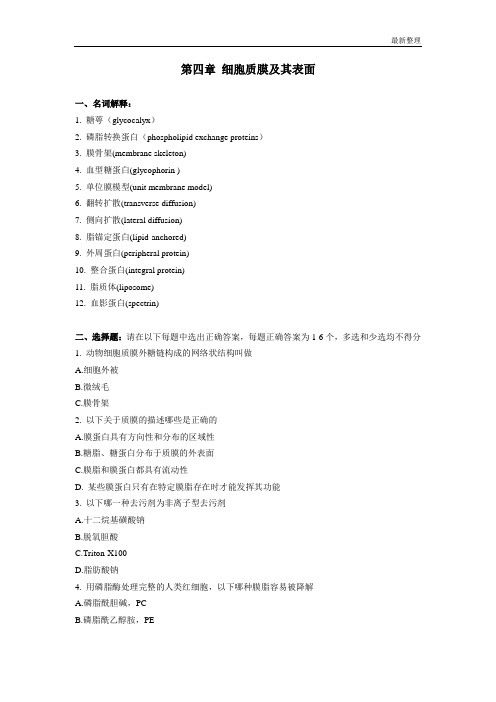
《逻辑与计算机设计基础》(原书第五版)课后习题答案-chapter04_solutions-5th
X Y
DA
Clock C
D
BX
Z
Clock C
2
Present state
AB
00 00 00 00 01 01 01 01 10 10 10 10 11 11 11 11
Inputs
XY
00 01 10 11 00 01 10 11 00 01 10 11 00 01 10 11
Next state
Input
1 0 011 0 1
1
1
1
0
Output
0 1 000 1 0
0
0
0
1
Next State 01 00 00 01 11 00 01 11 10 10 00
4-10.
00/0 11/1
01/0 10/1 11/0 0
00/0 01/1 10/0 11/1 01/0
00/1 1
01/1, 10/0
0
0
0 00
0 0
001
0
11
1 10
1 10
1 11
11
0
1
10
0
1
1 0
1
01
0
00
1
11
0
10
1
1
Nextt state state AB
A 0B 0
1
0
0 00 1
1 00 0
0 11 0
0 1
1
0 0
1
1 11 1
1 01 1
01
DA
B
1
A1 1
1
X
DDAA = AAXX+BBXX
现代移动通信蔡跃明第三版思考题与习题参考答案chapter_4
I (+1* +1)(+—1)第四章思考题与习题1. 移动通信对调制技术的要求有哪些?在移动通信中,由于信号传播的条件恶劣和快衰落的影响, 接收信号的幅度会发生急剧 的变化。
因此,在移动通信中必须采用一些抗干扰性能强、误码性能好、频谱利用率高的调 制技术,尽可能地提高单位频带内传输数据的比特速率以适用于移动通信的要求。
具体要求:① 抗干扰性能要强,如采用恒包络角调制方式以抗严重的多径衰落影响;② 要尽可能地提高频谱利用率;③ 占用频带要窄,带外辐射要小;④ 在占用频带宽的情况下,单位频谱所容纳的用户数要尽可能多;⑤ 同频复用的距离小;⑥ 具有良好的误码性能;⑦ 能提供较高的传输速率,使用方便,成本低。
2. 已调信号的带宽是如何定义的?信号带宽的定义通常都是基于信号功率谱密度 (PSD)的某种度量,对于已调(带通)信 号,它的功率谱密度与基带信号的功率谱密度有关。
假设一个基带信号:s(t) =Re{g(t)exp(j2二仁切其中的g(t)是基带信号,设g(t)的功率谱密度为P g (f),则带通信号的功率谱密度如下:P s (f )二1 P g (f - f c ) P g (-f - f c )l 4信号的绝对带宽定义为信号的非零值功率谱在频率上占据的范围; 最为简单和广泛使用的带宽度量是零点-零点带宽;半功率带宽定义为功率谱密度下降到一半时或者比峰值低 3dB 时的频率范围;联邦通信委员会 (FCC)采纳的定义为占用频带内有信号功率的99%。
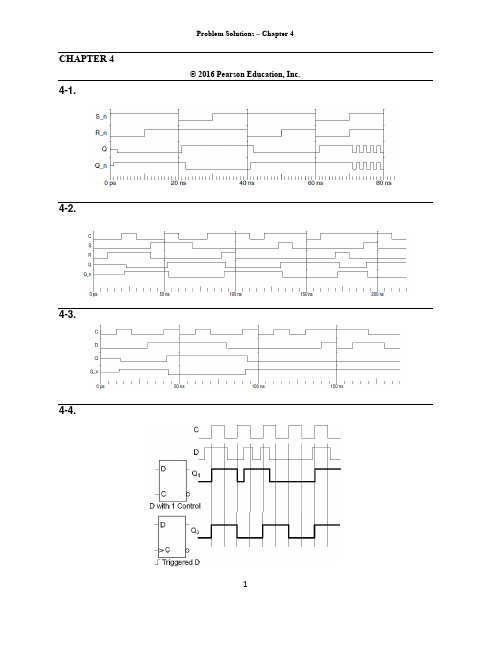
3. QPS K 、OQPSK 的星座图和相位转移图有何差异?如图所示QPSK相位星座图OPSK相位星座图QPSK信号的相位有90°突变和180°突变。
OQPSK信号的相位只有90°跳变,而没有180°的相位跳变。
4. QPSK和OQPSK的最大相位变化量分别为多少?各自有哪些优缺点?OPSK的最大相位变化量为1800, OPSK最大相位变化量为900。
电子科大-微机原理习题解答-chap4

Chapter44.1 阐述总线的概念。
计算机系统为什么需要采用总线结构?总线是计算机系统中的信息传输通道,由系统中各个部件所共享。
总线的特点在于公用性,总线由多条通信线路(线缆)组成采用总线结构,能:减少部件间连线的数量;扩展性好,便于构建系统;便于产品更新换代4.3 微机系统中总线层次化结构是怎样的?按总线所处位置可分为:片内总线、系统内总线、系统外总线。
按总线功能可分为:地址总线、数据总线、控制总线。
按时序控制方式可分为:同步总线、异步总线。
按数据格式可分为:并行总线、串行总线。
4.4 评价一种总线的性能有那几个方面?总线时钟频率、总线宽度、总线速率、总线带宽、总线的同步方式和总线的驱动能力等。
4.5 微机系统什么情况下需要总线仲裁?总线仲裁有哪几种?各有什么特点?总线仲裁又称总线判决,其目的是合理的控制和管理系统中多个主设备的总线请求,以避免总线冲突。
当多个主设备同时提出总线请求时,仲裁机构按照一定的优先算法来确定由谁获得对总线的使用权。
集中式(主从式)控制和分布式(对等式)控制。
集中式特点:采用专门的总线控制器或仲裁器分配总线时间,总线协议简单有效,总体系统性能较低。
分布式特点:总线控制逻辑分散在连接与总线的各个模块或设备中,协议复杂成本高,系统性能较高。
4.6总线传输方式有哪几种?同步总线传输对收发模块有什么要求?什么情况下应该采用异步传输方式,为什么?总线传输方式按照不同角度可分为同步和异步传输,串行和并行传输,单步和突发方式。
同步总线传输时,总线上收模块与发模块严格按系统时钟来统一定时收发模块之间的传输操作。
异步总线常用于各模块间数据传送时间差异较大的系统,因为这时很难同步,采用异步方式没有固定的时钟周期,其时间可根据需要可长可短。
4.7 AMBA总线定义了哪三种总线?他们各有什么特点?先进高性能总线AHB,先进系统总线ASB,先进外设总线APBAHB适用于高性能和高吞吐设备之间的连接,如CPU、片上存储器、DMA设备、DSP等。
Chapter04_Exercises

C. 识别、控制和跟踪需求的变化
D. 以上选项都不是
11. (
)需求工程师的任务是将所有利益相关者的信息进行分类以便允许决策者选择一
个相互一致的需求集。
A. 真
B. 假
12. 下面的(
)不是在项目启动阶段被提出的“与环境无关”的问题。
A. 成功的解决方案将带来什么样的经济收益?
B. 谁反对该项目?
C. 谁将为该项目付款?
2. 请指出下面需求描述存在的问题,并进行适当的修改。
(1) 系统用户界面友好。 (2) 系统运行时应该占用尽量少的内存空间。 (3) 即使在系统崩溃的情况下,用户数据也不能受到破坏。 (4) ATM 系统允许用户查询自己银行帐户的现存余额。 (5) ATM 系统应该快速响应用户的请求。 (6) ATM 系统需要检验用户存取的合法性。 (7) 所有命令的响应时间小于 1 秒;BUILD 命令的响应时间小于 5 秒。 (8) 软件应该用 JAVA 语言实现。 答案要点: (1) 问题:“友好”是不可验证的。
B. 每个指定系统的实现
C. 软件体系结构的元素
D. 系统仿真所需要的时间
9. 组织需求评审的最好方法是(
)。
A. 检查系统模型的错误
B. 让客户检查需求
C. 将需求发放给设计团队去征求意见
D. 使用问题列表检查每一个需求
10. 使用跟踪表有助于(
)。
A. 在后续的检查运行错误时调试程序
B. 确定算法执行的性能
(2) 需求分析:分析和综合所采集的信息,建立系统的详细逻辑模型。 (3) 需求规格说明:编写软件需求规格说明书,明确、完整和准确地描述已确定的需求。 (4) 需求验证:评审软件需求规格说明,以保证其正确性、一致性、完备性、准确性和清
管理会计(英文版)课后习题答案(高等教育出版社)chapter 4
管理会计(高等教育出版社)于增彪(清华大学)改编余绪缨(厦门大学)审校CHAPTER 4ACTIVITY-BASED COSTINGQUESTIONS FOR WRITING AND DISCUSSION1.Unit costs provide essential informationneeded for inventory valuation and prepara-tion of income statements. Knowing unit costs is also critical for many decisions such as bidding decisions and accept-or-reject special order decisions.2.Cost measurement is determining the dollaramounts associated with resources used in production. Cost assignment is associating the dollar amounts, once measured, with units produced.3.An actual overhead rate is rarely used be-cause of problems with accuracy and timeli-ness. Waiting until the end of the year to en-sure accuracy is rejected because of the need to have timely information. Timeliness of information based on actual overhead costs runs into difficulty (accuracy problems) because overhead is incurred nonuniformly and because production also may be non-uniform.4.For plantwide rates, overhead is first col-lected in a plantwide pool, using direct trac-ing. Next, an overhead rate is computed and used to assign overhead to products. 5.First stage: Overhead is assigned to produc-tion department pools using direct tracing, driver tracing, and allocation. Second stage: Individual departmental rates are used to assign overhead to products as they pass through the departments.6.Departmental rates would be chosen overplantwide rates whenever some depart-ments are more overhead intensive than others and if certain products spend more time in some departments than they do in others.7.Plantwide overhead rates assign overheadto products in proportion to the amount of the unit-level cost driver used. If the prod-ucts consume some overhead activities in different proportions than those assigned by the unit-level cost driver, then cost dis-tortions can occur (the product diversity factor). These distortions can be significant if the nonunit-level overhead costs represent a significant proportion of total overhead costs.8.Low-volume products may consume non-unit-level overhead activities in much greater proportions than indicated by a unit-levelcost driver and vice versa for high-volumeproducts. If so, then the low-volume prod-ucts will receive too little overhead and thehigh-volume products too much.9.If some products are undercosted and oth-ers are overcosted, a firm can make a num-ber of competitively bad decisions. For ex-ample, the firm might select the wrongproduct mix or submit distorted bids.10.Nonunit-level overhead activities are thoseoverhead activities that are not highly corre-lated with production volume measures. Ex-amples include setups, material handling,and inspection. Nonunit-level cost driversare causal factors—factors that explain theconsumption of nonunit-level overhead. Ex-amples include setup hours, number ofmoves, and hours of inspection.11.Product diversity is present whenever prod-ucts have different consumption ratios fordifferent overhead activities.12.An overhead consumption ratio measuresthe proportion of an overhead activity con-sumed by a product.13.Departmental rates typically use unit-levelcost drivers. If products consume nonunit-level overhead activities in different propor-tions than those of unit-level measures, thenit is possible for departmental rates to moveeven further away from the true consumptionratios, since the departmental unit-level ra-tios usually differ from the one used at theplant level.14.Agree. Prime costs can be assigned usingdirect tracing and so do not cause cost dis-tortions. Overhead costs, however, are notdirectly attributable and can cause distor-tions. For example, using unit-level activitydrivers to trace nonunit-level overhead costswould cause distortions.15.Activity-based product costing is an over-head costing approach that first assignscosts to activities and then to products. Theassignment is made possible through theidentification of activities, their costs, and theuse of cost drivers.16.An activity dictionary is a list of activitiesaccompanied by information that describeseach activity (called attributes)17. A primary activity is consumed by the finalcost objects such as products and custom-ers, whereas secondary activities are con-sumed by other activities (ultimately con-sumed by primary activities).18.Costs are assigned using direct tracing andresource drivers.19.Homogeneous sets of activities are pro-duced by associating activities that have thesame level and that can use the same driverto assign costs to products. Homogeneoussets of activities reduce the number of over-head rates to a reasonable level.20. A homogeneous cost pool is a collection ofoverhead costs that are logically related tothe tasks being performed and for whichcost variations can be explained by a singleactivity driver. Thus, a homogeneous pool ismade up of activities with the same process,the same activity level, and the same driver.21.Unit-level activities are those that occur eachtime a product is produced. Batch-level activi-ties are those that are performed each time abatch of products is produced. Product-levelor sustaining activities are those that areperformed as needed to support the variousproducts produced by a company. Facility-level activities are those that sustain a facto-ry’s general man ufacturing process.22.ABC improves costing accuracy wheneverthere is diversity of cost objects. There arevarious kinds of cost objects, with productsbeing only one type. Thus, ABC can be use-ful for improving cost assignments to costobjects like customers and suppliers. Cus-tomer and supplier diversity can occur for asingle product firm or for a JIT manufactur-ing firm.23.Activity-based customer costing can identifywhat it is costing to service different custom-ers. Once known, a firm can then devise astrategy to increase its profitability by focus-ing more on profitable customers, convertingunprofitable customers to profitable oneswhere possible, and “firing” customers thatcannot be made profitable.24.Activity-based supplier costing traces allsupplier-caused activity costs to suppliers.This new total cost may prove to be lowerthan what is signaled simply by purchaseprice.EXERCISES4–11.Quarter 1 Quarter 2 Q uarter 3 Quarter 4 Total Units produced 400,000 160,000 80,000 560,000 1,200,000 Prime costs $8,000,000 $3,200,000 $1,600,000 $11,200,000 $24,000,000 Overhead costs $3,200,000 $2,400,000 $3,600,000 $2,800,000 $12,000,000 Unit cost:Prime $20 $20 $20 $20 $20Overhead 8 15 45 5 10Total $28 $35 $65 $25 $30 2. Actual costing can produce wide swings in the overhead cost per unit. Thecause appears to be nonuniform incurrence of overhead and nonuniform production (seasonal production is a possibility).3. First, calculate a predetermined rate:OH rate = $11,640,000/1,200,000= $9.70 per unitThis rate is used to assign overhead to the product throughout the year.Since the driver is units produced, $9.70 would be assigned to each unit.Adding this to the actual prime costs produces a unit cost under normal cost-ing:Unit cost = $9.70 + $20.00 = $29.70This cost is close to the actual annual cost of $30.00.1. $13,500,000/3,600,000 = $3.75 per direct labor hour (DLH)2. $3.75 ⨯ 3,456,000 = $12,960,0003. Applied overhead $ 12,960,000A ctual overhead 13,600,000U nderapplied overhead $ 640,0004. Predetermined rates allow the calculation of unit costs and avoid the prob-lems of nonuniform overhead incurrence and nonuniform production asso-ciated with actual overhead rates. Unit cost information is needed throughout the year for a variety of managerial purposes.4–31. Predetermined overhead rate = $4,500,000/600,000 = $7.50 per DLH2. Applied overhead = $7.50 ⨯ 585,000 = $4,387,5003. Applied overhead $ 4,387,500Actual overhead 4,466,250Underapplied overhead $ (78,750)4. Unit cost:Prime costs $ 6,750,000Overhead costs 4,387,500Total $ 11,137,500Units ÷750,000Unit cost $ 14.851. Predetermined overhead rate = $4,500,000/187,500 = $24 per machine hour(MHr)2. Applied overhead = $24 187,875 = $4,509,0003. Applied overhead $ 4,509,000Actual overhead 4,466,250Overapplied overhead $ 42,7504. Unit cost:Prime costs $ 6,750,000Overhead costs 4,509,000Total $ 11,259,000Units ÷750,000Unit cost $ 15.01**Rounded5. Gandars needs to determine what causes its overhead. Is it primarily labordriven (e.g., composed predominantly of fringe benefits, indirect labor, and personnel costs), or is it machine oriented (e.g., composed of depreciation on machinery, utilities, and maintenance)? It is impossible for a decision to be made on the basis of the information given in this exercise.1. Predetermined rates:Drilling Department: Rate = $600,000/280,000 = $2.14* per MHrAssembly Department: Rate = $392,000/200,000= $1.96 per DLH*Rounded2. Applied overhead:Drilling Department: $2.14 ⨯ 288,000 = $616,320Assembly Department: $1.96 ⨯ 196,000 = $384,160Overhead variances:Drilling Assembly Total Actual overhead $602,000 $ 412,000 $ 1,014,000 Applied overhead 616,320 384,160 1,000,480 Overhead variance $ (14,320) over $ 27,840 under $ 13,520 3. Unit overhead cost = [($2.14 ⨯ 4,000) + ($1.96 ⨯ 1,600)]/8,000= $11,696/8,000= $1.46**Rounded1. Activity rates:Machining = $632,000/300,000= $2.11* per MHrInspection = $360,000/12,000= $30 per inspection hour*Rounded2. Unit overhead cost = [($2.11 ⨯ 8,000) + ($30 ⨯ 800)]/8,000= $40,880/8,000= $5.114–71. Yes. Since direct materials and direct labor are directly traceable to eachproduct, their cost assignment should be accurate.2. Elegant: (1.75 ⨯ $9,000)/3,000 = $5.25 per briefcaseFina: (1.75 ⨯ $3,000)/3,000 = $1.75 per briefcaseNote: Overhead rate = $21,000/$12,000 = $1.75 per direct labor dollar (or 175 percent of direct labor cost).There are more machine and setup costs assigned to Elegant than Fina. This is clearly a distortion because the production of Fina is automated and uses the machine resources much more than the handcrafted Elegant. In fact, the consumption ratio for machining is 0.10 and 0.90 (using machine hours as the measure of usage). Thus, Fina uses nine times the machining resources as Elegant. Setup costs are similarly distorted. The products use an equal number of setups hours. Yet, if direct labor dollars are used, then the Elegant briefcase receives three times more machining costs than the Fina briefcase.4–7 Concluded3. Overhead rate = $21,000/5,000= $4.20 per MHrElegant: ($4.20 ⨯ 500)/3,000 = $0.70 per briefcaseFina: ($4.20 ⨯ 4,500)/3,000 = $6.30 per briefcaseThis cost assignment appears more reasonable given the relative demands each product places on machine resources. However, once a firm moves to a multiproduct setting, using only one activity driver to assign costs will likely produce product cost distortions. Products tend to make different demands on overhead activities, and this should be reflected in overhead cost assign-ments. Usually, this means the use of both unit- and nonunit-level activity drivers. In this example, there is a unit-level activity (machining) and a non-unit-level activity (setting up equipment). The consumption ratios for each (using machine hours and setup hours as the activity drivers) are as follows:Elegant FinaMachining 0.10 0.90 (500/5,000 and 4,500/5,000)Setups 0.50 0.50 (100/200 and 100/200)Setup costs are not assigned accurately. Two activity rates are needed—one based on machine hours and the other on setup hours:Machine rate: $18,000/5,000 = $3.60 per MHrSetup rate: $3,000/200 = $15 per setup hourCosts assigned to each product:Machining: Elegant Fina$3.60 ⨯ 500 $ 1,800$3.60 ⨯ 4,500 $ 16,200Setups:$15 ⨯ 100 1,500 1,500Total $ 3,300 $ 17,700Units ÷3,000 ÷3,000Unit overhead cost $ 1.10 $ 5.90Activity dictionary:Activity Activity Primary/ ActivityName Description Secondary Driver Providing nursing Satisfying patient Primary Nursing hours care needsSupervising Coordinating Secondary Number of nurses nurses nursing activitiesFeeding patients Providing meals Primary Number of mealsto patientsLaundering Cleaning and Primary Pounds of laundry bedding and delivering clothesclothes and beddingProviding Therapy treatments Primary Hours of therapy physical directed bytherapy physicianMonitoring Using equipment to Primary Monitoring hours patients monitor patientconditions1. dCost of labor (0.75 ⨯ $40,000) $30,000Forklift (direct tracing) 6,000 Total cost of receiving $36,000 2. b3. a4. c5. dActivity rates (Questions 2–5):Receiving: $36,000/50,000 = $0.72 per partSetup: $60,000/300 = $200 per setupGrinding: $90,000/18,000 = $5 per MHrInspecting: $45,000/4,500 = $10 per inspection hour6. aOverhead rate = $231,000/20,000 = $11.55 per DLH Direct materials $ 850Direct labor 600Overhead ($11.55 ⨯ 50) 578*Total cost $ 2,028Units ÷100Unit cost $ 20.28*Rounded4–9 Concluded7. bDirect materials $ 850.00Direct labor 600.00Overhead:Setup 200.00 ($200 ⨯ 1)Inspecting 40.00 ($10 ⨯ 4)Grinding 100.00 ($5 ⨯ 20)Receiving 14.40 ($0.72 ⨯ 20) Total costs $ 1,804.40Units ÷100Unit cost $ 18.04**Rounded4–101. Unit-level: Testing products, inserting dies2. Batch-level: Setting up batches, handling wafer lots, purchasingmaterials, receiving materials3. Product-level: Developing test programs, making probe cards,engineering design, paying suppliers4. Facility-level: Providing utilities, providing space4–111. Unit-level activities: MachiningBatch-level activities: Setups and packing Product-level activities: ReceivingFacility-level activities: None2. Pools and drivers:Unit-levelPool 1:Machining $80,000Activity driver: Machine hoursBatch-levelPool 2:Setups $24,000Packing 30,000Total cost $54,000Product-levelPool 3:Receiving $18,000Activity driver: Receiving orders4–11 Concluded3. Pool rates:Pool 1: $80,000/40,000 = $2 per MHrPool 2: $54,000/300 = $180 per setupPool 3: $18,000/600 = $30 per receiving order 4. Overhead assignment:InfantryPool 1: $2 ⨯ 20,000 = $ 40,000Pool 2: $180 ⨯ 200 = 36,000Pool 3: $30 ⨯ 200 = 6,000Total $ 82,000Special forcesPool 1: $2 ⨯ 20,000 = $ 40,000Pool 2: $180 ⨯ 100 = 18,000Pool 3: $30 ⨯ 400 = 12,000Total $ 70,0004–121. Deluxe Percent Regular PercentPrice $900 100% $750 100% Cost 576 64 600 80 Unit gross profit $324 36% $150 20% Total gross profit:($324 ⨯ 100,000) $32,400,000($150 ⨯ 800,000) $120,000,0002. Calculation of unit overhead costs:Deluxe Regular Unit-level:Machining:$200 ⨯ 100,000 $20,000,000$200 ⨯ 300,000 $60,000,000 Batch-level:Setups:$3,000 ⨯ 300 900,000$3,000 ⨯ 200 600,000 Packing:$20 ⨯ 100,000 2,000,000$20 ⨯ 400,000 8,000,000 Product-level:Engineering:$40 ⨯ 50,000 2,000,000$40 ⨯ 100,000 4,000,000 Facility-level:Providing space:$1 ⨯ 200,000 200,000$1 ⨯ 800,000 800,000 Total overhead $ 25,100,000 $ 73,400,000 Units ÷100,000 ÷800,000 Overhead per unit $ 251 $ 91.75Deluxe Percent Regular Percent Price $900 100% $750.00 100%Cost 780* 87*** 574.50** 77***Unit gross profit $120 13%*** $175.50 23%***Total gross profit:($120 ⨯ 100,000) $12,000,000($175.50 ⨯ 800,000) $140,400,000*$529 + $251**$482.75 + $91.75***Rounded3. Using activity-based costing, a much different picture of the deluxe and regu-lar products emerges. The regular model appears to be more profitable. Per-haps it should be emphasized.4–131. JIT Non-JITSales a$12,500,000 $12,500,000Allocation b750,000 750,000a$125 ⨯ 100,000, where $125 = $100 + ($100 ⨯ 0.25), and 100,000 is the average order size times the number of ordersb0.50 ⨯ $1,500,0002. Activity rates:Ordering rate = $880,000/220 = $4,000 per sales orderSelling rate = $320,000/40 = $8,000 per sales callService rate = $300,000/150 = $2,000 per service callJIT Non-JITOrdering costs:$4,000 ⨯ 200 $ 800,000$4,000 ⨯ 20 $ 80,000Selling costs:$8,000 ⨯ 20 160,000$8,000 ⨯ 20 160,000Service costs:$2,000 ⨯ 100 200,000$2,000 ⨯ 50 100,000T otal $ 1,160,000 $ 340,000For the non-JIT customers, the customer costs amount to $750,000/20 = $37,500 per order under the original allocation. Using activity assignments, this drops to $340,000/20 = $17,000 per order, a difference of $20,500 per or-der. For an order of 5,000 units, the order price can be decreased by $4.10 per unit without affecting customer profitability. Overall profitability will decrease, however, unless the price for orders is increased to JIT customers.3. It sounds like the JIT buyers are switching their inventory carrying costs toEmery without any significant benefit to Emery. Emery needs to increase prices to reflect the additional demands on customer-support activities. Fur-thermore, additional price increases may be needed to reflect the increased number of setups, purchases, and so on, that are likely occurring inside the plant. Emery should also immediately initiate discussions with its JIT cus-tomers to begin negotiations for achieving some of the benefits that a JIT supplier should have, such as long-term contracts. The benefits of long-term contracting may offset most or all of the increased costs from the additional demands made on other activities.4–141. Supplier cost:First, calculate the activity rates for assigning costs to suppliers: Inspecting components: $240,000/2,000 = $120 per sampling hourReworking products: $760,500/1,500 = $507 per rework hourWarranty work: $4,800/8,000 = $600 per warranty hourNext, calculate the cost per component by supplier:Supplier cost:Vance Foy Purchase cost:$23.50 ⨯ 400,000 $ 9,400,000$21.50 ⨯ 1,600,000 $ 34,400,000 Inspecting components:$120 ⨯ 40 4,800$120 ⨯ 1,960 235,200 Reworking products:$507 ⨯ 90 45,630$507 ⨯ 1,410 714,870 Warranty work:$600 ⨯ 400 240,000$600 ⨯ 7,600 4,560,000 Total supplier cost $ 9,690,430 $ 39,910,070Units supplied ÷400,000 ÷1,600,000Unit cost $ 24.23* $ 24.94**RoundedThe difference is in favor of Vance; however, when the price concession is con sidered, the cost of Vance is $23.23, which is less than Foy’s component.Lumus should accept the contractual offer made by Vance.4–14 Concluded2. Warranty hours would act as the best driver of the three choices. Using thisdriver, the rate is $1,000,000/8,000 = $125 per warranty hour. The cost as-signed to each component would be:Vance Foy Lost sales:$125 ⨯ 400 $ 50,000$125 ⨯ 7,600 $ 950,000$ 50,000 $ 950,000 U nits supplied ÷ 400,000 ÷1,600,000I ncrease in unit cost $ 0.13* $ 0.59**RoundedPROBLEMS4–151. Product cost assignment:Overhead rates:Patterns: $30,000/15,000 = $2.00 per DLHFinishing: $90,000/30,000 = $3.00 per DLHUnit cost computation:Duffel BagsPatterns:$2.00 ⨯ 0.1 $0.20$2.00 ⨯ 0.2 $0.40Finishing:$3.00 ⨯ 0.2 0.60$3.00 ⨯ 0.4 1.20Total per unit $0.80 $1.602. Cost before addition of duffel bags:$60,000/100,000 = $0.60 per unitThe assignment is accurate because all costs belong to the one product.4–15 Concluded3. Activity-based cost assignment:Stage 1:Pool rate = $120,000/80,000 = $1.50 per transactionStage 2:Overhead applied:Backpacks: $1.50 ⨯ 40,000* = $60,000Duffel bags: $1.50 ⨯ 40,000 = $60,000*80,000 transactions/2 = 40,000 (number of transactions had doubled)Unit cost:Backpacks: $60,000/100,000 = $0.60 per unitDuffel bags: $60,000/25,000 = $2.40 per unit4. This problem allows the student to see what the accounting cost per unitshould be by providing the ability to calculate the cost with and without the duffel bags. With this perspective, it becomes easy to see the benefits of the activity-based approach over those of the functional-based approach. The activity-based approach provides the same cost per unit as the single-product setting. The functional-based approach used transactions to allocate accounting costs to each producing department, and this allocation probably reflects quite well the consumption of accounting costs by each producing department. The problem is the second-stage allocation. Direct labor hours do not capture the consumption pattern of the individual products as they pass through the departments. The distortion occurs, not in using transac-tions to assign accounting costs to departments, but in using direct labor hours to assign these costs to the two products.In a single-product environment, ABC offers no improvement in product cost-ing accuracy. However, even in a single-product environment, it may be poss-ible to increase the accuracy of cost assignments to other cost objects such as customers.4–161. Plantwide rate = $660,000/440,000 = $1.50 per DLHOverhead cost per unit:Model A: $1.50 ⨯ 140,000/30,000 = $7.00Model B: $1.50 ⨯ 300,000/300,000 = $1.502. Departmental rates:Department 1: $420,000/180,000 = $2.33 per MHr*Department 2: $240,000/400,000 = $0.60 per DLHDepartment 1: $420,000/40,000 = $10.50 DLHDepartment 2: $240,000/40,000 = $6.00 per MHrOverhead cost per unit:Model A: [($2.33 ⨯ 10,000) + ($0.60 ⨯ 130,000)]/30,000 = $3.38Model B: [($2.33 ⨯ 170,000) + ($0.60 ⨯ 270,000)]/300,000 = $1.86Overhead cost per unit:Model A: [($10.50 ⨯ 10,000) + ($6.00 ⨯ 10,000)]/30,000 = $5.50Model B: [($10.50 ⨯ 30,000) + ($6.00 ⨯ 30,000)]/300,000 = $1.65*Rounded numbers throughoutA common justification is that of using machine hours for machine-intensivedepartments and labor hours for labor-intensive departments. Using this rea-soning, the first set of departmental rates would be selected (machine hours for Department 1 and direct labor hours for Department 2).3. Calculation of pool rates:Driver Pool RateBatch-level pool:Setup and inspection Product runs $320,000/100 = $3,200 per runUnit-level pool:Machine andmaintenance Machine hours $340,000/220,000 = $1.545 per MHr Note: Inspection hours could have been used as an activity driver instead of production runs.Overhead assignment:Model BBatch-level:Setups and inspection$3,200 ⨯ 40 $ 128,000$3,200 ⨯ 60 $ 192,000Unit-level:Power and maintenance$1.545 ⨯ 20,000 30,900$1.545 ⨯ 200,000 309,000Total overhead $ 158,900 $ 501,000Units produced ÷30,000 ÷ 300,000Overhead per unit $ 5.30 $ 1.674. Using activity-based costs as the standard, we can say that the first set ofdepartmental rates decreased the accuracy of the overhead cost assignment (over the plantwide rate) for both products. The opposite is true for the second set of departmental rates. In fact, the second set is very close to the activity assignments. Apparently, departmental rates can either improve or worsen plantwide assignments. In the first case, D epartment 1’s costs are assigned at a 17:1 ratio which overcosts B and undercosts A in a big way.Yet, this is the most likely set of rates at the departmental level! This raises some doubt about the conventional wisdom regarding departmental rates.4–171. Labor and gasoline are driver tracing.Labor (0.75 ⨯ $120,000) $ 90,000 Time = Resource driverGasoline ($3 ⨯ 6,000 moves) 18,000 Moves = Resource driverDepreciation (2 ⨯ $6,000) 12,000 Direct tracingTotal cost $ 120,0002. Plantwide rate = $600,000/20,000= $30 per DLHUnit cost:DeluxePrime costs $80.00 $160Overhead:$30 ⨯ 10,000/40,000 7.50$30 ⨯ 10,000/20,000 15$87.50 $1753. Pool 1: Maintenance $ 114,000Engineering 120,000Total $ 234,000Maintenance hours ÷4,000Pool rate $ 58.50Note:Engineering hours could also be used as a driver. The activities are grouped together because they have the same process, are both product lev-el, and have the same consumption ratios (0.25, 0.75).Pool 2: Material handling $ 120,000Number of moves ÷6,000Pool rate $ 20Pool 3: Setting up $ 96,000Number of setups ÷80Pool rate $ 1,200Note: Material handling and setups are both batch-level activities but have dif-ferent consumption ratios.Pool 4: Purchasing $ 60,000Receiving 40,000Paying suppliersTotal $ 130,000Orders processed ÷750Pool rate $ 173.33Note:The three activities are all product-level activities and have the same consumption ratios.Pool 5: Providing space $ 20,000Machine hours ÷10,000Pool rate $ 2Note: This is the only facility-level activity.4. Unit cost:Basic Deluxe Prime costs $ 3,200,000 $ 3,200,000Overhead:Pool 1:$58.50 ⨯ 1,000 58,500$58.50 ⨯ 3,000 175,500 Pool 2:$20 ⨯ 2,000 40,000$20 ⨯ 4,000 80,000 Pool 3:$1,200 ⨯ 20 24,000$1,200 ⨯ 60 72,000 Pool 4:$173.33 ⨯ 250 43,333$173.33 ⨯ 500 86,665 Pool 5:$2 ⨯ 5,000 10,000$2 ⨯ 5,000 10,000 Total $ 3,375,833 $ 3,624,165Units produced ÷40,000 ÷20,000Unit cost (ABC) $ 84.40 $ 181.21Unit cost (traditional) $ 87.50 $ 175.00The ABC costs are more accurate (better tracing—closer representation of actual resource consumption). This shows that the basic model was over-costed and the deluxe model undercosted when the plantwide overhead rate was used.1. Unit-level costs ($120 ⨯ 20,000) $ 2,400,000Batch-level costs ($80,000 ⨯ 20) 1,600,000Product-level costs ($80,000 ⨯ 10) 800,000Facility-level ($20 ⨯ 20,000) 400,000Total cost $ 5,200,0002. Unit-level costs ($120 ⨯ 30,000) $ 3,600,000Batch-level costs ($80,000 ⨯ 20) 1,600,000Product-level costs ($80,000 ⨯ 10) 800,000Facility-level costs 400,000Total cost $ 6,400,000The unit-based costs increase because these costs vary with the number of units produced. Because the batches and engineering orders did not change, the batch-level costs and product-level costs remain the same, behaving as fixed costs with respect to the unit-based driver. The facility-level costs are fixed costs and do not vary with any driver.3. Unit-level costs ($120 ⨯ 30,000) $ 3,600,000Batch-level costs ($80,000 ⨯ 30) 2,400,000Product-level costs ($80,000 ⨯ 12) 960,000Facility-level costs 400,000Total cost $ 7,360,000Batch-level costs increase as the number of batches changes, and the costs of engineering support change as the number of orders change. Thus, batches and orders increased, increasing the total cost of the model.4. Classifying costs by category allows their behavior to be better understood.This, in turn, creates the ability to better manage costs and make decisions.1. The total cost of care is $1,950,000 plus a $50,000 share of the cost of super-vision [(25/150) ⨯ $300,000]. The cost of supervision is computed as follows: Salary of supervisor (direct) $ 70,000Salary of secretary (direct) 22,000Capital costs (direct) 100,000Assistants (3 ⨯ 0.75 ⨯ $48,000) 108,000Total $ 300,000Thus, the cost per patient day is computed as follows:$2,000,000/10,000 = $200 per patient day(The total cost of care divided by patient days.) Notice that every maternity patient—regardless of type—would pay the daily rate of $200.2. First, the cost of the secondary activity (supervision) must be assigned to theprimary activities (various nursing care activities) that consume it (the driver is the number of nurses):Maternity nursing care assignment:(25/150) ⨯ $300,000 = $50,000Thus, the total cost of nursing care is $950,000 + $50,000 = $1,000,000.Next, calculate the activity rates for the two primary activities:Occupancy and feeding: $1,000,000/10,000 = $100 per patient dayNursing care: $1,000,000/50,000 = $20 per nursing hour。
扎维模拟CMOS集成电路设计第四章习题

I SS 1103 0.72V 4 0.383510 50 W p Cox L 3
Vout max 3 0.72 2.28V Vout , swing 2Vout max Vout min 22.28 0.673 3.214 V
Chapter 4 习题
4.11
Cox
0 ox
tox
8.851014 F / cm 3.9 7 2 3 . 835 10 F / cm 9 109 m
cm2 F 4 A nCox 350 3.835107 1 . 34225 10 V s cm2 V2 cm2 F 4 A pCox 100 3.835107 0 . 3835 10 V s cm2 V2
b. VDD 0.8V时,M 3截止,Vout 0, AV 0 VDD 0.8V时,M 3导通,M1工作在线性区,VDD ,Vout , AV 当VDD 上升到一定值时,M1进入饱和区。
VinCM 1.2V时,满足M1工作在饱和区的最小电 源电压为 VDD min VinCM VTH 1 VGS 3 1.2 0.7 1.607 2.107V
2 I D1 VGS 1 Vod 1 VTH 1 0.7 W nCox L 1 2 0.25103 0.7 0.893 V 4 1.3422510 100
VinCM min VodSS VGS 1 0.273 0.893 1.166 V
a. VinCMmin VodSS VGS1 VinCMmax VDD VGS3 VTH1
Introduction to Management Science 5th Edition, 课后习题答案 Chapter 4
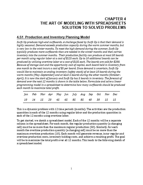
CHAPTER 4 THE ART OF MODELING WITH SPREADSHEETSSOLUTION TO SOLVED PROBLEMS4.S1Production and Inventory Planning ModelSurfs U p p roduces h igh-‐end s urfboards. A c hallenge f aced b y S urfs U p i s t hat t heir d emand i s highly s easonal. D emand e xceeds p roduction c apacity d uring t he w arm s ummer m onths, b ut is v ery l ow i n t he w inter m onths. T o m eet t he h igh d emand d uring t he s ummer, S urfs U ptypically p roduces m ore s urfboards t han a re n eeded i n t he w inter m onths a nd t hen c arries inventory i nto t he s ummer m onths. T heir p roduction f acility c an p roduce a t m ost 50 b oards per m onth u sing r egular l abor a t a c ost o f $125 e ach. U p t o 10 a dditional b oards c an b e produced b y u tilizing o vertime l abor a t a c ost o f $135 e ach. T he b oards a re s old f or $200. Because o f s torage c ost a nd t he o pportunity c ost o f c apital, e ach b oard h eld i n i nventory f rom one m onth t o t he n ext i ncurs a c ost o f $5 p er b oard. S ince d emand i s u ncertain, S urfs U p would l ike t o m aintain a n e nding i nventory (safety s tock) o f a t l east 10 b oards d uring t he warm m onths (May–September) a nd a t l east 5 b oards d uring t he o ther m onths (October–April). I t i s n ow t he s tart o f J anuary a nd S urfs U p h as 5 b oards i n i nventory. T he f orecast o f demand o ver t he n ext 12 m onths i s s hown i n t he t able b elow. F ormulate a nd s olve a l inear programming m odel i n a s preadsheet t o d etermine h ow m any s urfboards s hould b e p roduced each m onth t o m aximize t otal p rofit.Jan Feb Mar Apr May Jun July Aug Sep Oct Nov Dec10 14 15 20 45 65 85 85 40 30 15 15This i s a d ynamic p roblem w ith 12 t ime p eriods (months). T he a ctivities a re t he p roduction quantities i n e ach o f t he 12 m onths u sing r egular l abor a nd t he p roduction q uantities i n each o f t he 12 m onths u sing o vertime l abor.To g et s tarted, w e s ketch a s preadsheet m odel. E ach o f t he 12 m onths w ill b e a s eparate column i n t he s preadsheet. F or e ach m onth, t he r egular p roduction q uantity (a c hanging cell) m ust b e n o m ore t han t he m aximum r egular p roduction (50). S imilarly, f or e ach month t he o vertime p roduction q uantity (a c hanging c ell) m ust b e n o m ore t han t he maximum o vertime p roduction (10). E ach m onth w ill g enerate r evenue, i ncur r egular a nd overtime p roduction c osts, i nventory h olding c osts, a nd a chieve a r esulting p rofit. T he g oal will b e t o m aximize t he t otal p rofit o ver a ll 12 m onths. T his l eads t o t he f ollowing s ketch o f a s preadsheet m odel.The e nding i nventory e ach m onth w ill e qual t he s tarting i nventory (the g iven s tartinginventory f or J anuary, o r t he p revious m onth’s e nding i nventory f or f uture m onths) p lus a ll production (regular a nd o vertime) m inus t he f orecasted s ales. T he e nding i nventory a t t he end o f e ach m onth m ust b e a t l east t he m inimum s afety s tock l evel. T he r evenue w ill e qual the s elling p rice t imes f orecasted s ales. T he r egular (or o vertime) p roduction c ost w ill b e the r egular (or o vertime) p roduction q uantity t imes t he u nit r egular (or o vertime)production c ost. T he h olding c ost w ill e qual t he e nding i nventory t imes t he u nit h olding cost. T he m onthly p rofit w ill b e r evenue m inus b oth p roduction c osts m inus h olding c ost. Finally, t he t otal p rofit w ill b e t he s um o f t he m onthly p rofits. T he f inal s olved s preadsheet, formulas, a nd S olver i nformation a re s hown b elow.Unit Cost (Reg)Unit Cost (OT)Selling Price Holding Cost Starting Inventory<=Max Regular <=Max OTForecasted Sales Ending Inventory>=Safety StockThe v alues i n R egularProduction (C10:N10) a nd O TProduction (C14:N14) s how h ow m anysurf b oards S urfs U p s hould p roduce e ach m onth s o a s t o a chieve t he m aximum p rofit o f $31,150.Set Objective Cell: TotalProfit To: MaxBy Changing Variable Cells:RegularProduction, OTProduction Subject to the Constraints:RegularProduction <= MaxRegular OTProduction <= MaxOTEndingInventory >= SafetyStock Solver Options:Make Variables Nonnegative Solving Method: Simplex LP4.S2Aggregate Planning: Manpower Hiring/Firing/TrainingCool P ower p roduces a ir c onditioning u nits f or l arge c ommercial p roperties. D ue t o t he l owcost a nd e fficiency o f i ts p roducts, t he c ompany h as b een g rowing f rom y ear t o y ear. A lso, d ue to s easonality i n c onstruction a nd w eather c onditions, p roduction r equirements v ary f rommonth t o m onth. C ool P ower c urrently h as 10 f ully t rained e mployees w orking i nmanufacturing. E ach t rained e mployee c an w ork 160 h ours p er m onth a nd i s p aid a m onthly wage o f $4000. N ew t rainees c an b e h ired a t t he b eginning o f a ny m onth. D ue t o t heir l ack o f initial s kills a nd r equired t raining, a n ew t rainee o nly p rovides 100 h ours o f u seful l abor i n their f irst m onth, b ut a re s till p aid a f ull m onthly w age o f $4000. F urthermore, b ecause o f required i nterviewing a nd t raining, t here i s a $2500 h iring c ost f or e ach e mployee h ired. A fter one m onth, a t rainee i s c onsidered f ully t rained. A n e mployee c an b e f ired a t t he b eginning o f any m onth, b ut m ust b e p aid t wo w eeks o f s everance p ay ($2000). O ver t he n ext 12 m onths, Cool P ower f orecasts t he l abor r equirements s hown i n t he t able b elow. S ince m anagement anticipates h igher r equirements n ext y ear, C ool P ower w ould l ike t o e nd t he y ear w ith a t l east 12 f ully t rained e mployees. H ow m any t rainees s hould b e h ired a nd/or w orkers f ired i n e ach month t o m eet t he l abor r equirements a t t he m inimum p ossible c ost? F ormulate a nd s olve a linear p rogramming s preadsheet m odel.Jan Feb Mar Apr May Jun Jul Aug Sep Oct Nov Dec 1600 2000 2000 2000 2800 3200 3600 3200 1600 1200 800 800This i s a d ynamic p roblem w ith 12 t ime p eriods (months). T he a ctivities a re t he n umber o fworkers t o h ire a nd f ire i n e ach o f t he 12 m onths.To g et s tarted, w e s ketch a s preadsheet m odel. E ach o f t he 12 m onths w ill b e a s eparate column i n t he s preadsheet. F or e ach m onth, t here a re c hanging c ells f or b oth t he n umber o f workers h ired a nd f ired. B ased o n t he v alues o f t hese c hanging c ells, w e c an d etermine t he number o f t rainees a nd t rained e mployees. T he n umber o f l abor h ours g enerated b y t he employees m ust b e a t l east t he r equired l abor h ours e ach m onth. F inally, l abor c osts (for trainees a nd t he t rained w orkforce), h iring c ost, a nd s everance p ay l eads t o a t otal m onthly cost. T he g oal w ill b e t o m inimize t he t otal c ost o ver a ll 12 m onths. T his l eads t o t he following s ketch o f a s preadsheet m odel.Labor Monthly WageHiring Cost Severance PayLabor Hours/Trainee/MonthLabor Hours/Trained Worker/MonthStarting Trained WorkforceMinimum to Start the TraineesNext YearTrained Employees >=Labor Hours Available>=Required Labor HoursWhen a n e mployee i s f irst h ired, h e o r s he i s a t rainee f or o ne m onth b efore b ecoming afully-‐trained e mployee. T herefore, t he n umber o f t rainees (row 14) i s e qual t o t he n umber of w orkers h ired i n t hat m onth, w hile t he n umber o f t rained e mployees (row 15) i s t henumber o f t rained e mployees a nd t rainees f rom t he p revious m onth m inus a ny e mployee that i s f ired. T he l abor h ours a vailable i n e ach m onth e quals t he s umproduct o f t he l abor hours p rovided b y e ach t ype o f w orker (trained o r t rainees) w ith t he n umber o f e ach t ype of e mployee. T he l abor c osts i n e ach m onth a re t he m onthly w age m ultiplied b y t he number o f e mployees. T he h iring c ost i s t he u nit h iring c ost m ultiplied b y t he n umber o f workers h ired. T he s everance p ay i s t he u nit s everance c ost m ultiplied b y t he n umber o f workers f ired. T hen, t he t otal m onthly c ost i s t he s um o f t he l abor c osts, h iring c ost, a nd severance p ay. F inally, t he t otal c ost w ill b e t he s um o f t he m onthly c osts. F or a rbitrary values o f w orkers h ired a nd f ired e ach m onth, t his l eads t o t he f ollowing s preadsheet.The S olver i nformation i s s hown b elow, f ollowed b y t he s olved s preadsheet.Thus, W orkersHired (C11:N11) s hows t he n umber o f w orkers C ool P ower s hould h ire e achmonth a nd W orkersFired (C12:N12) s hows t he n umber o f w orkers C ool P ower s hould f ire each m onth s o a s t o a chieve t he m inimum T otalCost (O26) o f $787,500.Solver ParametersSet Objective Cell: TotalCost To: MinBy Changing Variable Cells: WorkersHired, WorkersFired Subject to the Constraints:N15 >= MinimumToStartNewYearLaborHoursAvailable >= RequiredLaborHours WorkersHired = integer WorkersFired = integer Solver Options:Make Variables Nonnegative Solving Method: Simplex LP。
- 1、下载文档前请自行甄别文档内容的完整性,平台不提供额外的编辑、内容补充、找答案等附加服务。
- 2、"仅部分预览"的文档,不可在线预览部分如存在完整性等问题,可反馈申请退款(可完整预览的文档不适用该条件!)。
- 3、如文档侵犯您的权益,请联系客服反馈,我们会尽快为您处理(人工客服工作时间:9:00-18:30)。
DC-AC变换器(无源逆变电路)一、学习目的:通过本章的学习,学者可以了解逆变器的电路结构、分类、特点及主要性能指标;对三种基本变换方式——方波变换、阶梯波变换、正弦波变换,有一定的认识;可以理解采用各种变换方式的逆变器的工作原理;了解空间矢量PWM控制的基本原理。
二、主要内容:1、基本概念DC-AC变换器是指能将一定幅值的直流输入电压(或电流)变换成一定幅值、一定频率的交流输出电压(或电流),并向无源负载(如电机、电炉、或其它用电器等)供电的电力电子装置,又称为无源逆变电路,常简称作逆变器(Inverter)。
完成直流电压变换的逆变器称为电压型逆变器,而完成直流电流变换的逆变器则称为电流型逆变器。
2、变换方式的分类(1)方波变换方式逆变器的交流输出有两种基本调制方式:脉冲幅值调制(PAM-Pluse Amplitude Modulation)和单脉冲调制(SPM-Single Pluse Modulation)。
所谓脉冲幅值调制(PAM)是指:逆变器的输出频率可由180°方波或120°方波(如图4-3b 所示)的周期来控制,而逆变器输出基波的幅值则由输出方波的幅值即逆变器直流侧电压(或电流)的幅值来控制。
显然,采用PAM控制方式时,其方波的导通角恒定(180°方波或120°方波)。
所谓的单脉冲调制(SPM)是指:逆变器的输出频率仍由方波的周期来控制,而逆变器输出基波的幅值则由逆变器输出方波的导通角进行控制,即可使导通角在0°~180°范围调节。
显然,采用SPM控制方式时,逆变器输出方波的幅值即逆变器直流侧电压(或电流)的幅值恒定。
(2)阶梯波变换方式(3)斩控调制方式:是指逆变器输出的调制脉冲幅值固定不变,而逆变器中的功率管以一定的控制规律进行调制。
斩控调制方式主要有以下二类即:①脉冲宽度调制(PWM);②脉冲频率调制(PFM)3、逆变器的分类(1)按直流侧储能元件的性质,逆变器可分为电压型逆变器(VSI-Voltage Source Inverter)和电流型逆变器(CSI-Current Source Inverter)。
(2)按逆变器输出波形的不同,逆变器可分为方波逆变器、阶梯波逆变器、以及正弦波逆变器等。
(3)按逆变器功率电路结构形式的不同,逆变器可分为半桥逆变器、全桥逆变器、推挽式逆变器等。
(4)按逆变器功率电路的功率器件的不同,逆变器可分为半控型逆变器和全控型逆变器。
(5)按逆变器输出频率的不同,逆变器可分为工频逆变器、中频逆变器以及高频逆变器。
(6)按逆变器输出交流电的相数的不同,逆变器可分为单相逆变器、三相逆变器以及多相逆变器。
(7)按逆变器输入、输出是否隔离,逆变器可分为隔离型逆变器和非隔离型逆变器。
(8)按逆变器输出电平的不同,逆变器可分为两电平逆变器和多电平逆变器。
4、逆变器的性能指标谐波系数HF、总谐波畸变系数THD、畸变系数DF、最低次谐波LOH等。
5、电压型逆变器(1)特点:①直流侧有足够大的储能电容元件,从而使其直流侧呈现出电压源特性,即稳态时的直流侧电压近似不变。
②逆变器输出的电压波形为方波或方波脉冲,并且该电压波形与负载无关。
③逆变器输出的电流波形则取决于负载,且输出电流的相位随负载功率因数的变化而变化。
④逆变器输出电压的控制可以通过PAM (脉冲幅值调制)和PWM(脉冲宽度调制)两种基本控制方式来实现。
(2)分类:依据电压型逆变器的控制方式和结构的不同,电压型逆变器主要可分为方波型、阶梯波型、正弦波型(PWM型)三类。
(3)电压型方波逆变器本章主要讨论电压型单相全桥方波逆变器、电压型单相半桥方波逆变器、带中心抽头变压器的电压型单相推挽式方波逆变器、电压型三相桥式方波逆变器.1)电压型单相全桥方波逆变器:34这种电压型单相全桥方波逆变器的输出波形控制主要有脉冲幅值调制(PAM)和单脉冲调制(SPM)两类,而单脉冲调制又包含对称单脉冲调制和移相单脉冲调制。
电压型单相全桥方波逆变器采用脉冲幅值调制(PAM)时,其主电路的四个功率管采用180°互补控制模式,这样逆变器输出的电压为180°导电的交流方波电压,其方波电压幅值即为逆变器的直流电压幅值。
采用对称单脉冲调制时,每半个输出周期对称改变一次逆变器的开关状态,并通过调整方波脉冲的宽度来控制逆变器输出电压的基波大小。
采用移相单脉冲调制时,单相全桥逆变器四个功率管驱动信号均为180°方波,并且负载一端上下桥臂的驱动信号相位固定,而负载另一端上下桥臂的驱动信号相位可移动。
调节超前桥臂与滞后桥臂间的相角θ,就可以调节单相全桥逆变器的输出方波宽度,从而控制逆变器输出电压的基波幅值。
2)电压型三相桥式方波逆变器U逆变器每相的方波变换可采用180°和120°两种方波调制方式,即所谓的180°导电方式和120°导电方式。
所谓180°导电方式是指三相桥式逆变器每相的方波变换采用180°方波调制方式,要求逆变器中功率管的驱动信号为180°方波,每相的上下桥臂均采用180°互补控制模式。
相邻相的桥臂驱动信号相位互差120°,任何时刻有且只有三个桥臂导电,或两个上桥臂一个下桥臂导电,或一个上桥臂两个下桥臂导电。
所谓120°导电方式是指三相桥式逆变器每相的方波变换采用120°方波调制方式,要求逆变器中功率管的驱动信号为120°方波,每相的上下桥臂均采用120°控制且有60°导通间隙。
相邻相的桥臂驱动信号相位互差120°,任何时刻有且只有两个桥臂导电,即一个上桥臂和一个下桥臂导电。
(5)电压型正弦波逆变器要求输出正弦波电压的电压型PWM逆变器,常称为电压型正弦波逆变器。
这种电压型正弦波逆变器一般应具备以下特点:①逆变器的直流电压可采用结构简单的不控整流电路;②利用单一的功率电路及其控制,可同时调整输出频率和输出电压,动态响应快;③由于输出电压的谐波频率主要分布在开关频率及其以上频段,因而输出谐波含量低。
1)单相电压型正弦波逆变器34单相电压型正弦波逆变器,可采用三种SPWM控制方案,即单极性SPWM控制、双极性SPWM控制以及倍频单极性SPWM控制。
所谓单极性SPWM控制是指逆变器的输出脉冲具有单极性特征。
即当输出正半周时,输出脉冲全为正极性脉冲;而当输出负半周时,输出脉冲全为负极性脉冲。
为此,必须采用使三角载波极性与正弦调制波极性相同的所谓单极性三角载波调制。
所谓双极性SPWM控制是指逆变器的输出脉冲具有双极性特征。
即无论输出正、负半周,输出脉冲全为正、负极性跳变的双极性脉冲。
当采用基于三角载波调制的双极性SPWM 控制时,只须采用正、负对称的双极性三角载波即可。
所谓倍频单极性SPWM控制是指:逆变器输出脉冲的调制频率是载波频率的两倍,并且输出脉冲具有单极性特征。
倍频单极性SPWM控制有调制波反相和载波反相两种PWM 控制模式。
2)三相电压型正弦波逆变器U三相电压型正弦波逆变器,可采用多种SPWM控制方案即:三相双极性SPWM控制、提高电压利用率的鞍形调制波SPWM控制以及既能提高电压利用率又能降低开关损耗的综合优化SPWM控制等。
三相双极性SPWM控制是三相电压型正弦波逆变器基本的SPWM控制方案,这种控制方案对每相桥臂采用以上讨论的双极性SPWM控制,即三相桥臂采用同一个三角载波信号,而三相桥臂的调制波则采用三相对称的正弦波信号。
进行傅立叶分析,若定义逆变器输出线电压的基波幅值与逆变器直流电压之比为电压型逆变器的电压利用率,显然,三相双极性SPWM控制时的正弦波逆变器电压利用率(约为0.866)较180°导电型控制时的方波逆变器电压利用率(约为1.1)低。
因此,在不增加SPWM 输出谐波的同时,为了提高SPWM控制时的电压利用率,可以采用鞍形调制波SPWM控制和综合优化SPWM控制。
三、重难点内容:1、电压型单相全桥方波逆变器的结构,工作过程和控制原理2、单相电压型正弦波逆变器的结构,工作过程和控制原理3、空间矢量PWM控制基本原理4、晶闸管三相全桥(串联二极管式)电流型方波逆变器的结构,工作过程和控制原理四、课后习题4.4什么是电压型逆变电路?什么是电流型逆变电路?二者各有什么特点?答:按照逆变电路直流侧电源性质分类,直流侧是电压源的逆变器称为电压型逆变电路,直流侧是电流源的逆变电路称为电流型逆变电路。
电压型逆变电路的主要特点是:1)直流侧有足够大的储能电容元件,从何使其直流侧呈现出电压源的特性,即稳态时的直流侧电压近似不变2)逆变器输出的电压波形为方波或方波脉冲,并且该电压波形与负载无关3)逆变器输出的电流波形则取决于负载,且输出电流的相位随负载功率因数的变化而变化4)逆变器输出电压的控制可以通过脉冲幅值调制(PAM)和脉冲宽度调制(PWM)两种基本的控制方式电流型逆变电路的主要特点是:1)直流侧有足够大的储能电感元件,从何使其直流侧呈现出电流源的特性,即稳态时的直流侧电流近似不变2)逆变器输出的电流波形为方波或方波脉冲,并且该电流波形与负载无关3)逆变器输出的电压波形则取决于负载,且输出电压的相位随负载功率因数的变化而变化4)逆变器输出电流的控制可以通过脉冲幅值调制(PAM)和脉冲宽度调制(PWM)两种基本的控制方式4.5电压型逆变电路中反馈二极管的作用是什么?为什么电流型逆变电路中没有反馈二极管?答:在电压型逆变电路中,当交流侧为阻感负载时需要提供无功功率,直流侧电容起到缓冲无功能量的作用。
为了给交流侧向直流侧反馈的无功能量提供通道,逆变桥各臂都并联了反馈二极管。
当输出交流电压和电流的极性相同时,电流经电路中的可控开关器件流通,而当输出电压电流极性相反时,由反馈二极管提供电流通道。
在电流型逆变电路中,直流电流极性是一定的,无功能量由直流侧电感来缓冲。
当需要从交流侧向直流侧反馈无功能量时,电流不反向,依然经电路中的可控开关器件流通,因此不需要并联反馈二极管。
4.8试分析采用120°导电方式的电压型三相桥式方波逆变电路的工作过程。
答:参照图4-12的电压型三相桥式逆变器电路结构和图4-14电压型三相桥式逆变器120°导电方式时的相关波形进行分析:采用120°导电方式的电压型逆变器在任何时刻有且只有两个桥臂导电,即一个上桥臂一个下桥臂导电,且相邻序号功率管的驱动信号相位互差60°。
假设VT1和VT6先导通,输出电压Uan为Ud/2,Ubn为-Ud/2,Ucn为0,因此输出电压Uab为Ud,Ubc为-Ud/2,Uca为-Ud/2;然后VT1和VT2导通,输出电压Uan为Ud/2,Ubn为0,Ucn 为-Ud/2,因此输出电压Uab为Ud/2,Ubc为Ud/2,Uca为-Ud; 然后VT2和VT3导通,输出电压Uan为0,Ubn为Ud/2,Ucn为-Ud/2,因此输出电压Uab为-Ud/2,Ubc为Ud,Uca为-Ud/2; 然后VT3和VT4导通,输出电压Uan为-Ud/2,Ubn为Ud/2,Ucn为0,因此输出电压Uab为-Ud,Ubc为Ud/2,Uca为Ud/2; 然后VT4和VT5导通,输出电压Uan为-Ud/2,Ubn为0,Ucn为Ud/2,因此输出电压Uab为-Ud/2,Ubc为-Ud/2,Uca为Ud; 然后VT5和VT6导通,输出电压Uan为0,Ubn为-Ud/2,Ucn为Ud/2,因此输出电压Uab为Ud/2,Ubc为-Ud,Uca为Ud/2。