Kinematic Analysis by Analytical(解析的)
机械原理英文词汇
机械原理英文词汇黄清世周传喜编长江大学机械学院Chapter 1 Introduction第一章绪论1.mechanism 机构2.kinematical element 运动学元件3.link 构件4.cam 凸轮5.gear 齿轮6.belt 带7.chain 链8.internal-combustion engine 内燃机9.slider-crank mechanism 曲柄滑块机构10.piston 活塞11.connecting rod 连杆12.crankshaft 曲轴13.frame 机架14.pinion 小齿轮15.cam mechanism 凸轮机构16.linkage 连杆机构17.synthesis 综合Chapter 2 Structure analysis of mechanisms第二章机构的结构分析1. structural analysis 结构分析2. planar mechanisms 平面机构3. planar kinematical pairs 平面运动副4. mobile connection 可动连接5. transmit 传输6. transform 转换7. pair element 运动副元素8. higher pair 高副9. revolute pair 转动副10. sliding pair ,prismatic pair 移动副11. gear pair 齿轮副12. cam pair 凸轮副13. screw pair 螺旋副14. spherical pair 球面副15. surface contact 面接触16. kinematical chain 运动链17. closed chain 闭式链18. open chain 开式链19. driving links 驱动件20. driven links 从动件21. planar mechanism. 平面机构22. spatial mechanism 空间机构23. The kinematical diagram of a mechanism机构运动简图24. schematic diagram 草图25. kinematical dimensions 运动学尺寸26. fixed pivot 固定铰链27. pathway 导路28. guide bar 导杆29. profiles 轮廓30. the actual cam contour 凸轮实际廓线.31. polygon 多边形32. route of transmission 传递路线33. structural block diagram 结构框图34. Degree of Freedom (DOF) 自由度35. constraints 约束36. common normal 公法线37. compound hinge 复合铰链38. gear-linkage mechanism 齿轮连杆机构40. passive DOF 局部自由度41. redundant constraint 虚约束42. The composition principle and structural analysis组成原理与结构分析43. the basic mechanism 基本机构44. Assur groups 阿苏尔杆组45. inner pair 内副46. outer pairs 外副.47. composition principle of mechanism 机构组成原理48. kinematical determination 运动确定性Chapter 3 kinematic analysis of mechanicsms 第三章机构的运动分析1. velocity 速度2. acceleration 加速度3. parameter 参数3. graphical method 图解法4. analytical method 解析法5. experimental method 实验法6. instant center 瞬心7. classification of instant centers 瞬心的分类8. absolute instantaneous center 绝对瞬心9. relative instantaneous center 相对瞬心10. the method of instantaneous center 瞬心法11. the Aronhold-Kennedy theorem阿朗浩尔特-肯尼迪定理(即三心定理)12. the four-bar linkage 四杆机构13. inversion of the slider-crank导杆机构(曲柄滑块机构的倒置机构) 14. complex mechanism 复杂机构,多杆机构Chapter 5 Efficiency and Self-lock ofMachines第五章机械效率和自锁1.pure-slide pair 移动副2.helical pair 螺旋副3.Coulomb’s law 库仑定律4.coefficient of friction 摩擦系数5.rest friction 静摩擦6.kinetic friction 动摩擦7.vee-slot V型槽8.equivalent coefficient of friction 当量摩擦系数9.frictional angle 摩擦角10.equivalent frictional angle 当量摩擦角11.lead angle 导程角12.moment of couple 力偶矩13.clearance 间隙14.frictional circle 摩擦圆15.thrust bearing 推力轴承16.drive work 驱动功17.effective work 有效功18.lost work 损耗功19.ideal machine 理想机械20.serial structure 串联结构21.parallel structure 并联结构22.parallel-serial structure 混联结构23.jack 千斤顶24.self-lock 自锁Chapter 6 Balancing of Machinery第六章机械的平衡1. Vibration 振动2. Frequency 频率3. Resonant 共振4. Amplitudes 振幅5. Balancing of rotors 转子6. Rigid rotors 刚性转子7. Flexible rotors 柔性转子8. Balancing of mechanisms 机构的平衡9. Disk-like rotor 盘状转子10.Non-disk rigid rotor 非盘状转子11.the shaking force 振动力12.the shaking moment 振动力矩13.Balancing of Disk-like Rotors 盘状转子的平衡14.static imbalance 静不平衡15.static balancing machine 静平衡机16.the mass-radius product 质径积17.dynamically unbalanced 动不平衡18.balance planes 平衡基面19.Dynamic balancing machine 动平衡机20.Unbalancing Allowance 许用不平衡量Chapter 7 Motion of Mechanical Systemsand Its Regulation第七章机械系统的运转及其调节1. Periodic speed fluctuation 周期性波动2. punching machine 冲床3. Motion Equation of a Mechanical System机械系统的运动方程4. General Expression of the Equation of Motion运动方程的一般表达式5. the kinetic energy 动能6. the moment of inertia 转动惯量7. Dynamically Equivalent Model of a Mechanical System等效动力学模型8. the equivalent moment of inertia 等效转动惯量9. the equivalent moment of force 等效力矩10.the equivalent link 等效构件11.Pump 泵12.Blower 鼓风机13.Flywheel 飞轮Chapter 8 Planar Linkage Mechanicsms第八章平面连杆机构1.four-bar linkage 四杆机构2.crank-rocker mechanism 曲柄摇杆机构3.double-crank mechanism 双曲柄机构4.double-rocker mechanism 双摇杆机构5.Crashof’s criterion 格拉索夫判据6.Condition for having a crank 有曲柄的条件7.slider-crank mechanism 曲柄滑块机构8.offset distance 偏距9.offset slider-crank mechanism 偏置曲柄滑块机构10.in-line slider-crank mechanism 对心曲柄滑块机构11.rotating guide-bar mechanism. 转动导杆机构12.oscillating guide-bar mechanism 摆动导杆机构13.double rotating block mechanism 双转块机构14.crank and oscillating block mechanism 曲柄摇块机构15.variations 变异16.inversions 倒置17.transmission angle 传动角18.dead point 死点19.imbalance angle 极位夹角20.time ratio 行程速比系数21.quick-return mechanism 急回机构22.pressure angle 压力角23.toggle positions 肘节位置24.oldham coupling 联轴器25.flywheel 飞轮26.clamping device 夹具27.dimensional synthesis 尺度综合28.function generation 函数发生器29.body guidance 刚体导引30.path generation 轨迹发生器Chapter 9 Cam Mechanisms第九章凸轮机构1. contour 轮廓2. Follower 从动件3. Plate cam(or disc cam) 盘形凸轮4. Translating cam 移动凸轮5. Three-dimensional cam 空间凸轮6. cylindrical cam 圆柱凸轮7. Translating follower 直动从动件8. Oscillating follower 摆动从动件9. Camshaft 凸轮轴10.in-line translating follower 对心直动从动件11.offset translating follower 偏置直动从动件12.Knife-edge follower 尖底从动件13.Roller follower 滚子从动件14.Flat-faced follower 平底从动件15.Force-closed cam mechanism 力封闭凸轮机构16.Form-closed cam mechanism 形封闭凸轮机构17.Lift 行程18.cam angle for rise 推程角19.cam angle for outer dwell 远休止角20.cam angle for return 回程角21.cam angle for inner dwell 近休止角22.the quasi-velocity 类速度23.the quasi-acceleration 类加速度24.Constant Velocity Motion Curve 等速运动规律25.rigid impulse 刚性冲击26.Constant Acceleration and Deceleration Motion Curve等加速等减速运动规律27.soft impulse 柔性冲击29.Cosine Acceleration Motion Curve (Simple Harmonic Motion Curve) 余弦加速度运动规律(简谐运动规律)30.Sine Acceleration Motion Curve (Cycloid Motion Curve)正弦加速度运动规律(摆线运动规律)31.3-4-5 Polynomial Motion Curve 3-4-5多项式运动规律bined Motion Curves 组合运动规律33.the cam contour 实际廓线34.the pitch curve 理论廓线35.prime circle 基圆36.the common normal 公法线37.positive offset 正偏置38.negative offset 负偏置39.outer envelope 外包络线40.inner envelope 内包络线41.The locus of the centre of the milling cutter铣刀中心轨迹42.Pressure Angle 压力角43.acute angle 锐角44.the normal 法线45.The allowable pressure angle 许用压力角46.Radius of Curvature 曲率半径47.Cusp 尖点48.Undercutting 根切49.The angular lift 角行程50.interference 干涉Chapter 10 Gear Mechanisms第十章齿轮机构1. constant transmission ratio 定传动比2. planar gear mechanisms 平面齿轮机构3. spatial gear mechanisms 空间齿轮机构4. external gear pair 外齿轮副5. internal gear pair 内齿轮副6. rack and pinion 齿条和齿轮7. spur gear 直齿轮8. helical gear 斜齿轮9. double helical gear 人字齿轮10.spur rack 直齿条11.helical rack 斜齿条12.bevel gear mechanism 圆锥齿轮机构13.crossed helical gears mechanism 螺旋齿轮机构14.worm and worm wheel mechanism 蜗杆蜗轮机构15.Fundamentals of Engagement of Tooth Profiles齿廓啮合基本定律16.the pitch point 节点17.the pitch circle 节圆18.conjugate profiles 共轭齿廓19.transmission ratio 传动比20.involute gear 渐开线齿轮21.the radius of base circle 基圆半径22.generating line 发生线23.unfolding angle 展角24.table of involute function 渐开线函数表25.gearing 啮合26.standard involute spur gears 标准渐开线直齿轮27.the facewidth 齿宽28.addendum circle (or tip circle) 齿顶圆29.dedendum circle (or root circle) 齿根圆30.arbitrary circle 任意圆31.the tooth space 齿槽32.the spacewidth 齿槽宽33.the pitch 齿距,周节34.the reference circle 分度圆35.module 模数36.addendum 齿顶高37.dedendum 齿根高38.tooth depth 齿全高39.the coefficient of addendum 齿顶高系数40.the coefficient of bottom clearance 顶隙系数41.bottom clearance 顶隙42.the normal tooth 正常齿43.the shorter tooth 短齿44.base pitch 基圆齿距,基节45.normal pitch 法向齿距,法节46.conjugated point 共轭点47.proper meshing conditions 正确啮合条件48.working pressure angle 啮合角49.the backlash 齿侧间隙50.the bottom clearance 顶隙51.the reference centre distance 标准中心距52.contact ratio 重合度53.the actual working profile 实际工作齿廓54.the actual line of action 实际啮合线55.manufacturing methods of involute profiles渐开线齿廓的加工方法56.form cutting 仿形法57.generating cutting 展成法或范成法58.disk milling cutter 盘形铣刀59.end milling cutter 指状铣刀60.broach 拉刀ling machines. 铣床62.rack-shaped shaper cutter 齿条插刀63.shaping 插齿64.hobbing 滚齿65.rack-shaped cutter 齿条型刀具the 车床67.cutter Interference 根切68.corrected gears 变位齿轮69.the modification coefficient 变位系数70.positively modified 正变位71.negatively modified 负变位72.the gearing equation without backlash 无侧隙啮合方程73.involute helicoids 渐开线螺旋面74.the transverse plane 端面75.the normal plane 法面78.the transverse contact ratio 端面重合度79.the overlap ratio 轴向重合度80.the virtual gear 当量齿轮81.the virtual number of teeth 当量齿数82.axial thrust 轴向推力83.worm gearing 蜗杆传动84.righthanded 右旋85.lefthanded 左旋86.ZA-worm 阿基米德蜗杆87.involute helicoid worms ----ZI-worm 渐开线蜗杆88.arc-contact worms -----ZC-worm 圆弧齿蜗杆89.enveloping worm 包络蜗杆90.The number of threads 头数91.bevel gears 圆锥齿轮92.back cone 背锥93.virtual gear 当量齿轮94.the reference cone 分度圆锥95.sector gear 扇形齿轮96.the outer cone distance 外锥距97.the reference cone angle 分度圆锥角98.The apexes 锥顶99.The dedendum angle 齿根角100.dedendum cone angle 齿根圆锥角Chapter 11 Gear Trains第十一章轮系1. gear train with fixed axes 定轴轮系2. epicyclical gear train 周转轮系3. elementary epicyclical gear trains 基本周转轮系4. combined gear trains 复合轮系5. planet gear 行星轮6. planet carrier 行星架,系杆,转臂7. sun gears 太阳轮,中心轮8. differential gear train 差动轮系9. the train ratio of a gear train 轮系传动比10.idle wheels 惰轮11.converted gear train 转化轮系12.the efficiency of the gear train 轮系效率13.branching transmission 分路传动14.the brake 刹车片15.the clutch 离合器16.negative mechanism 负号机构17.positive mechanism 正号机构18.train ratio condition 传动比条件19.concentric condition 同心条件20.assembly condition 装配条件21.planetary reducer with small tooth difference少齿差行星减速器22.cycloidal-pin wheel planetary gearing摆线针轮行星传动23.harmonic drive gearing 谐波传动Chapter 12 Other Common Mechanisms 第十二章其它常用机构1. ratchet mechanism 棘轮机构2. pawl 棘爪3. intermittent motion 间歇运动4. geneva mechanism 槽轮机构5. external geneva mechanism 外槽轮机构6. internal geneva mechanism 内槽轮机构7. geneva rack mechanism 齿条槽轮机构8. spherical geneva mechanisms 球面槽轮机构9. the ratio k between motion time and dwell time运动与停歇时间比k10.Cam-Type Index Mechanisms 凸轮式间歇运动机构11.Cylindrical Cam Index Mechanisms圆柱凸轮式间歇运动机构12.Universal Joints 万向联轴节13.The Single Universal Joint 单万向联轴节14.The Double Universal Joint 双万向联轴节15.Screw Mechanisms 螺旋机构16.single-threadscrew mechanisms 单螺旋机构17.Double-thread screw mechanisms 复式螺旋机构18.Index cam mechanism 分度凸轮机构19.Geared linkages 齿轮连杆机构Chapter 13 Creative Design of Mechanism Systems 第十三章机械系统的创新设计1. prototype machine 样机2. Working cycle diagrams 工作循环图3. reference link 定标件4. Circular working cycle diagram 圆工作循环图5. Rectilinear working cycle diagram 矩形工作循环图6. Rectangular coordinate working cycle diagram直角坐标式工作循环图the coefficient travel speed variation K 行程速比系数crank acute angle (imbalance angle) θ极位夹角differential gear train 差动轮系planetary gear train 行星轮系magnitude and direction (大小和方向)compound hinge 复合铰链passive DOF 局部自由度redundant constraint 虚约束offset cam mechanism 偏置凸轮机构pressure angle 压力角base circle 基圆instant centre 瞬心transmission angle 传动角。
机械英语
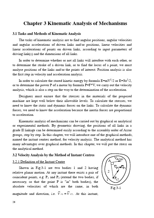
Chapter 3 Kinematic Analysis of Mechanisms3.1 Tasks and Methods of Kinematic AnalysisThe tasks of kinematic analysis are to find angular positions, angular velocities and angular accelerations of driven links and/or positions, linear velocities and linear accelerations of points on driven links, according to input parameters of driving link(s) and the dimensions of all links.In order to determine whether or not all links will interfere with each other, or to determine the stroke of a driven link, or to find the locus of a point, we must analyse positions of the links and/or the points of interest. Position analysis is also the first step in velocity and acceleration analysis.In order to calculate the stored kinetic energy by formula E=mV 2/2 or E=J ω2/2, or to determine the power P of a motor by formula P=F*V , we carry out the velocity analysis, which is also a step on the way to the determination of the acceleration.Designers must ensure that the stresses in the materials of the proposed machine are kept well below their allowable levels. To calculate the stresses, we need to know the static and dynamic forces on the links. To calculate the dynamic forces, we need to know the acceleration because the inertia forces are proportional to acceleration.Kinematic analysis of mechanisms can be carried out by graphical or analytical or experimental methods. By geometric drawing, the positions of all links in a grade II linkage can be determined easily according to the assembly order of Assur groups, step by step. In this chapter, we will introduce one of the graphical methods, named the instant centres method, for velocity analysis. The analytical method has many advantages over graphical methods. In this chapter, we will put the stress on the analytical method.3.2.1 Definition of the Instant CentreShown in Fig.3-1 are two bodies 1 coincident points, e.g. P 1 and P 2necessary, so that the point P is "in" both absolute velocities of which are the magnitude and direction, i.e. V V P P 12=. At this instant,Fig.3-1there is no relative velocity between this pair of coincident points, i.e.V VP P P P1221==0. Thus, at this instant, either link will have pure rotation relative to the other link about the point. This pair of coincident points with the same velocities is defined as the instantaneous centre of relative rotation, or more briefly the instant centre, denoted as P12or P21. If one of links is the frame, the instant centre is called an absolute instant centre, otherwise, a relative instant centre. The absolute instant centre is the zero-velocity point on a moving link, but its acceleration may not be zero.At the position shown in Fig.3-1, the two links rotate relative to each other about the instant centre P12. So any other pair of coincident points, e.g. A1 and A2, will have relative velocities, i.e. V A1A2 and V A2A1. The directions of V A1A2 and V A2A1 are perpendicular to PA. Therefore, if the direction of the relative velocity of a pair of coincident points, e.g. A1 and A2, is known, then the instant centre must lie somewhere on the normal to the relative velocity passing through the coincident point A.3.2.2 Number of Instant Centres of a MechanismEach pair of links i and j has an instant centre and P ij is identical to P ji. Thus the number N of instant centres of a mechanism with K links isNK K=-*()12Note: The frame is included in the number K.3.2.3 Location of the Instant Centre of Two Links Connected by a Kinematic Pair (1) Revolute pairIf two links 1 and 2 are connected by a revolute pair, as shown in Fig.3-2(a), the centre of the revolute pair is obviously the instant centre P12 or P21.(2) Pure-rolling pairThe pure-rolling pair is a special case of a higher pair, as shown in Fig.3-2(b). There is no slipping between the two contacting points A1and A2, i.e. V A1A2=V A2A1=0. Thus the point of contact A is the instant centre P12or P21. Kinematically, the transmission between a pair of gears is equivalent to rolling without slipping between a pair of circles. So the contact point of the two pitch circles of the gears 1 and 2 is the instant centre P12 for the gears 1 and 2, as shown in Fig.3-2(c).(3) Sliding pairAs can be seen in Fig.3-2(d), relative translation is equivalent to relative rotation about a point located at infinity in either direction perpendicular to the guide-way. Therefore, the instant centre of the two links connected by a sliding pair lies at infinity in either direction perpendicular to the guide-way.The instant centres mentioned so far are called observable instant centres and should be located and labeled before any others are found.(4) Higher pair (rolling & sliding pair)Shown in Fig.3-2(e) are two links 1 and 2 connected by a higher pair. Their contact point is point A. The direction of relative velocities, V A1A2and V A2A1, between A1 and A2 must be along the common tangent. Otherwise there will be a relative velocity component along the common normal n-n which will make the. According to the theorem of three centres, the three instant centres P12 , P13 and P23 must lie on a straight line. This theorem can be proved as follows.Suppose that the positions of P12 and P13 are known, as shown in Fig.3-3. Let us consider any point, e.g. point C, outside the line P12P13. Since P12(A) is the instant centre of the links 1 and 2, the link 2 rotates relative to the link 1 about the point A. So V C2C1⊥AC. Similarly, V C3C1⊥BC. Since V C2=V C1+V C2C1, thenV C2C1=V C2-V C1. Similarly, V C3C1=V C3-V C1. Obviously, for any point Coutside the line P12P13, the directions of the vectors V C2C1 and V C3C1 are not thesame, i.e. VC2C1 ≠V C3C1.(V C2-V C1) ≠(V C3-V C1) from which obtains C2≠C3. Hence, according to be the instant centre P 23 between the links 2 and3. In other words, any point outside the straightline P 12P 13 cannot be the instant centre P 23. Thus the theorem of three centres is derived: the three instant centres of any three independent links in general plane motion must lie on a common straight line.3.2.5 Applications of Instant CentresExample 3-1For the four-bar mechanism shown in Fig.3-4, the angular velocity ω1 of crank 1 is given. For the position shown,(1) locate all instant centres for the mechanism,(2) find the ratio ω3 /ω1 of the angular velocity of link 3 to that of link 1,(3) find the velocity V F of point F on link 2.Solution:(1)There are sixcentres in this four-bar mechanism. In order to should first try to locate observable instant centres. There are four instant centres (P 14, P 12, P 23 and P 34) and two unobservable instantcentres (P 13 and P 24) in this mechanism. According to the theorem of three centres, P 13 will lie not only on the line P 14P 34, but also on the line P 12P 23. Since P 23 is at infinity perpendicular to the guiding bar 2, line P 12P 23 passes through the point P 12 Fig.3-3 Fig.3-4and is perpendicular to BF. Hence the intersection E of the lines P14P34 and P12P23 is the instant centre P13.Similarly, line P23P34 passes through the point P34 and is perpendicular to BF, the intersection G of the lines P12P14 and P34P23 is the instant centre P24. Thus it can be seen that it is usual to apply the theorem of three centres twice to determine two lines, the intersection of which will be the unobservable instant centre. Instant centres P14, P34and P24are absolute instant centres, while the others are relative instant centres.(2) In order to find ω3 for the given ω1, we should take advantage of the frame 4. Their three instant centres(P34, P13, P14) lie on a common straight line. The moving links 1 and 3 rotate relative to the frame 4 about the absolute instant centres P14(A) and P34(D) respectively. In link 1, V E1=ω1*L AE. In link 3, V E3=ω3*L DE. (Extend the two links, if necessary, so that the point E is "in" both links.) Since the point E is the instant centre P13between the links 1 and 3, V E1=V E3.Therefore, ω1*L AE=ω3*L DE from which i31=ω3/ω1= L AE/L DE =P14P13/P34P13. The lengths of L AE and L DE are measured directly from the kinematic diagram of the mechanism. The direction of ω3 is counter-clockwise at this instant.From above, it is shown that the ratio ωi /ωj of angular velocities between any two moving links i and j is equal to the inverse ratio of the two distances between the relative instant centre P i j and two absolute instant centres P f i and P f j , that is,ωωijfj ijfi ijP PP P=----------------------------------------------------------------------(3-1)where the subscript f represents the frame! If the relative instant centre P ij lies between the two absolute instant centres P fi and P fj, then the directions of ωi and ωj are different. Otherwise, the directions of ωi and ωj are the same.(3) Since the links 2 and 3 are connected by a sliding pair, they cannot rotate relative to each other. Thus, ω2 =ω3 =ω1*L AE/L ED. Since P24 is the absolute instant centre, the link 2 rotates (relative to the frame 4) about the point P24(G) at this instant. Therefore, V F=ω2*L GF. Its direction is perpendicular to GF, as shown in Fig.3-4. Note: Although the velocity of the point P24(G) is zero, its acceleration is not zero.Example 3-2In the cam mechanism with translating roller follower shown in Fig.3-5, the cam is a circular disk. Supposing that the angular velocity ω1 of the cam is known,the velocity V 2the position shown.Solution: As mentioned in passive DOF. The velocity of change if the roller is welded normal n-n through the point of contact C. Accordingto the theorem of three centres, P 12 must lie on the straight line connecting P 13 and P 23. Since the links 2 and 3 are connected by a sliding pair and their instant centre P 23 is at infinity perpendicular to the guide way, the line P 13P 23 passes through P 13 and is perpendicular to the guide way. Thus the intersection B of the common normal n-n and the line P 13P 23 is the instant centre P 12 and V B1 =V B2. Note: Neither the centre O of the circle nor the contact point C is the instant centre P 12. On the cam 1, V B1 =ω1*L AB . Since the follower 2 is translating, all points on the follower 2 have the same velocity 2. So V 2 =V B2 =V B1 =ω1*L AB .Example 3-3In Fig.3-6, gear 3 rolls onrack 4 without slipping. velocity 1 of slider 1 is velocity V D is to be found.Solution: In order to find the point on the gear 3, angular velocity ω3 of the gear 3 should be found first. As mentioned before, in order to find ω3 of the gear 3 for the given velocity V 1 of the slider 1, we always take advantage of the Fig.3-5 Fig.3-6frame 4. Thus we should try to locate the three instant centres, P34, P14and P13, between the three links 1, 3 and the frame 4. The gear 3 rolls on the fixed rack 4 without slipping. So the contact point C is their instant centre P34. P14 lies at infinity perpendicular to AB(not AC!). P13 must lie on both lines P14P34 and P23P12. So the intersection E of the lines P14P34and P23P12is the instant centre P13between the links 1 and 3. Therefore V E3 =V E1. Since the slider 1 is translating, V1 =V E1 =V E3=ω3*L CE. Thus ω3 =V1/L CE from which V D =ω3*L CD =V1*L CD /L CE. The direction is as shown in Fig.3-6.3.2.6 Advantages and Disadvantages of the Method of Instant CentresThe method of instant centres offers an excellent tool in the velocity analysis of simple mechanisms. However, in a complex mechanism, some instant centres may be difficult to find. In some cases they will lie off the paper. Lastly, it should be pointed out that an instant centre, in general, changes its location on both links during motion. The acceleration of the instant centre is not zero(except for fixed pivots). Therefore, the instant centre method cannot be used in acceleration analysis.3.3 Kinematic Analysis by Analytical MethodsIn graphical methods, none of the information obtained for the first position of the mechanism will be applicable to the second position or to any others. The kinematic diagram of the mechanism must be redrawn for each position of the driver. This is very tedious if a mechanism is to be analyzed for a complete cycle. Furthermore, the accuracy of the graphical solution is limited.In contrast, once the analytical solution is derived using an analytical method, it can be evaluated on a computer for different dimensions and/or at different positions with very little effort. The accuracy of the solution far surpasses that required for mechanical design problems. Thus, in this chapter we will put stress on the analytical method. Graphical methods can be used if necessary as a check on the analytical solutions.There exist many kinds of analytical methods for kinematic analysis of linkages. The kinematic analysis of a multi-bar linkage mechanism seems to be a hard task at first sight. However, it becomes easier if the Assur-group method is used. As mentioned in Sec.2.5, most linkage mechanisms are built up by adding one or more commonly used Assur groups to the basic mechanism. Since the DOF of an Assur group is zero, Assur groups have kinematic determination. That is, the motions of all links in an Assur group can be determined so long as the motions of all outer pairs are known. Taking this fact into account, one can set up subroutinesin advance for some commonly used Assur groups. Then the kinematic analysis of a multi-bar linkage mechanism is reduced to two simple steps: first, dividing the mechanism into Assur groups and secondly, calling the corresponding subroutine for each Assur group according to the type and the assembly order of the Assur group. This method is called the Assur-group method for kinematic analysis.In the next sections, we will set up some commonly used kinematic analysis subroutines before analyzing a six-bar linkage mechanism.3.3.1 The LINK Subroutineand acceleration of a point A (i.e. X A, Y A, (V A)X, (V A)Y(a A)Yacceleration of link AB(i.e. θ, ω, ε) and the length (L ABlink AB are known, as shown in Fig.3-7. The Xcomponents of position, velocity and acceleration of point B (i.e.Fig.3-7X B, Y B, (V B)X, (V B)Y, (a B)X, (a B)Y) can be calculated as follows.In a Cartesian co-ordinate system,X B=X A+L AB * cos(θ) and Y B=Y A+L AB * sin(θ) Differentiating the above position analysis formulae with respect to time, the formulae for velocity analysis can be derived.(V B)X=(V A)X - L AB * sin(θ)*ωand (V B)Y=(V A)Y +L AB*cos(θ)*ωDifferentiating again, the formulae for analyzing the acceleration of the point B can be derived.(a B)X= (a A)X - L AB* sin(θ)*ε - L AB* cos(θ)*ω2and(a B)Y = (a A)Y + L AB* cos(θ)*ε -L AB* sin(θ)*ω2These six formulae can be programmed in a subroutine. In the TRUE BASIC computer language, any subroutine must begin with statement SUB subroutine-name(table of parameters) and end with statement END SUB. Let us name the subroutine LINK. Then the LINK subroutine is as follows:SUB LINK(XA,YA,V AX,V AY,AAX,AAY,Q,W,E,LAB,XB,YB,VBX,VBY,ABX,ABY) LET XB=XA+LAB*COS(Q)LET YB=YA+LAB*SIN(Q)LET VBX=V AX-LAB*SIN(Q)*WLET VBY=V AY+LAB*COS(Q)*WLET ABX=AAX-LAB*SIN(Q)*E-LAB*COS(Q)*W^2LET ABY=AAY+LAB*COS(Q)*E-LAB*SIN(Q)*W^2END SUBEvery evaluating statement must begin with LET. In order to facilitate the understanding of the program, parameters should have easily-recognized names. For example, (V A )X is named V AX. The table of the parameters corresponds to (X A , Y A , (V A )X , (V A )Y , (a A )X , (a A )Y , θ, ω, ε, L AB , X B , Y B , (V B )X , (V B )Y , (a B )X , (a B )Y ). After the subroutine is called, the kinematic parameters of the point B will be known. 3.3.2 The RRR SubroutineIn the RRR group shown inthe kinematic parameters of the points A and C and the lengths of links AB and CB are known. The positions, angular velocities and calculated as follows. When X A , Y A , X C , Y C , L AB determined, there are two assembly modesfor this group, as shown in Fig.3-8, one in solid lines and the other in dashed lines. On the link CB, X B =X C +L CB *cos(θCB ) and Y B =Y C +L CB *sin(θCB )On the link AB, X B =X A +L AB *cos(θAB ) and Y B =Y A +L AB *sin(θAB )Combining these two sets of equations, one obtains:X L X L Y L Y L C CB CB A AB AB CCB CB A AB AB +=++=+⎧⎨⎩*cos()*cos()*sin()*sin()θθθθ ----------------------------(3-2) There are two unknowns, θAB and θCB , in this set of equations. Since there are two assembly modes for this group, there will be two sets of solutions. Although some mathematical skill can be used to solve the above trigonometric non-linear equations to obtain two sets of formulae for θAB and θCB , the calculation process is tedious and the formulae derived would be very complicated. It is hard to judge which set of formulae corresponds to a specific assembly mode. The following is a simple method to overcome this difficulty.(a) L AC =()()X X Y Y C A C A -+-22(b) cos θAC =(X C -X A )/L AC and sin θAC =(Y C -Y A )/L ACThe subroutine may be used for any combinations of the positions of points A Fig.3-8and C. Note that sin θAC may not be equal to ()12-cos θAC since sin θAC may be negative. The magnitude of θAC can be calculated according to the values of both cos θAC and sin θAC by the ANGLE function in TRUE BASIC. Note again that θ may not be equal to ATN(sin θ/cos θ) since θ may be greater than π/2 and less than 3*π/2, whereas the value obtained from the ATN function is only from -π/2 to +π/2. Note: θAC is 180︒ different from θCA .(c) cos θBAC =()()L L L L L AB AC CB AB AC 2222+-/** Since 180︒>θBAC >0︒, sin θBAC =()12-cos θBAC . If L AC >(L AB +L CB ), then cos θBAC >1. This means that the distance L AC between the two outer points is greater than the sum of L AB and L CB . If L AC <|L AB -L CB |, then cos θBAC <(-1) and the distance L AC is less than the difference between L AB and L CB . In these cases, the RRR dyad can not be assembled. The calculation of ()12-cos θBAC will fail and computation will be stopped.(d) As mentioned before, there are two assembly modes for the RRR group. For the assembly mode shown by solid lines, θAB =θAC -θBAC . During motion of the mechanism, the assembly mode does not change as a result of change in position.(e) X B =X A +L AB *cos(θAB ) and Y B =Y A +L AB *sin(θAB )(f) cos θCB =(X B -X C )/L CB and sin θCB =(Y B -Y C )/L CBThe magnitude of θCB can be calculated according to the values of both cos θCB and sin θCB by the ANGLE function in TRUE BASIC.Velocity analysis can be progressed only after the position analysis is finished. The angular velocities, ωAB and ωCB , of the links AB and CB can be found by differentiating Eqs.(3-2) with respect to time. ()*sin()*()*sin()*()*cos()*()*cos()*V L V L V L V L C X CB CB CB A X AB AB AB C YCB CB CB A Y AB AB AB -=-+=+⎧⎨⎩θωθωθωθω -------------(3-3) Both velocity and acceleration equations of a grade II Assur group are dualistic linear equations. The explicit expressions for ωAB and ωCB can be found easily by solving the two equations simultaneously.By differentiating Eqs.(3-3) with respect to time, another set of dualistic linear equations with two unknowns, i.e. the angular accelerations εAB and εCB ofthe links AB and CB, is derived. The explicit expressions for εAB and εCB can be found easily by solving the two equations simultaneously.Using the above explicit expressions, not the equations, the subroutine named RRR for kinematic analysis of the RRR group can be written as follows:SUB RRR(XA, YA, V AX, V AY, AAX, AAY, XC, YC, VCX, VCY, ACX, ACY, LAB, LCB, QAB, WAB, EAB, QCB, WCB, ECB)LET LAC=SQR((XC-XA)^2+(YC-YA)^2)LET COSQAC=(XC-XA)/LACLET SINQAC=(YC-YA)/LACLET QAC=ANGLE(COSQAC,SINQAC)LET COSQBAC=(LAB^2+LAC^2-LCB^2)/(2*LAB*LAC)LET SINQBAC=SQR(1-COSQBAC^2)LET QBAC=ANGLE(COSQBAC,SINQBAC)LET QAB=QAC-QBACLET XB=XA+LAB*COS(QAB)LET YB=YA+LAB*SIN(QAB)LET COSQCB=(XB-XC)/LCBLET SINQCB=(YB-YC)/LCBLET QCB=ANGLE(COSQCB,SINQCB).......................................LET WAB=....................LET WCB=.............................................................LET EAB=.......................LET ECB=.......................END SUBAttention should be paid to the sequence of the revolute's letters in the table of the parameters when the subroutine is called. For this subroutine, the three letters A, B and C are arranged in CCW.3.3.3 The RPR SubroutineShown in Fig.3-9(a) is an RPR Assur group. The revolutes A and C are outer revolute pairs. The eccentric AB is perpendicular to guide-bar BD. The kinematic parameters of the centers, A and C, of the two outer revolute pairs and the length of eccentric AB are known. There are two assembly modes for this group. One is shown in solid lines, the other in dashed lines. The angular position, angular velocity and angular acceleration of the guide-bar BD (θBD, ω, ε) can be calculated as follows:L AC =()()X X Y Y C A C A -+-22, cos θAC =(X C -X A )/L AC ,sin θAC =(Y C -Y A )/L AC ,L BC =L L AC AB 22-.If L AC <L AB , then the group can not be assembled. In this case, the calculation ofL L AC AB 22- will fail and the computation will be stopped.θACB =tg L L AB BC -⎛⎝ ⎫⎭⎪1, θBD = θAC +M* θACB , and θAB = θBD -M*π/2where M is the coefficient of the assembly mode. For the solid mode, M=+1. For the dashed mode, M=-1. During motion of the mechanism, the assembly mode does not change as a result of change in position. We can determine the value of M according to the assembly mode at any angle of the driver.From Fig.3-9, we haveX X L X L L Y Y L Y L L C B BC BD A AB AB BC BD CB BC BD A AB AB BC BD =+=++=+=++⎧⎨⎩cos()cos()cos()sin()sin()sin()θθθθθθ Differentiating the above equations with respect to time results in--+=--+=-⎧⎨⎩()cos()*()()()sin()*()()Y Y VLBC V V X X VLBC V V C A BD C X A XCA BD C Y A Y ωθωθ -------------------(3-4) where VLBC is the derivative of L BC with respect to time.Solving the dualistic linear equations Eqs.(3-4) simultaneously, the explicit(a) (b) Fig.3-9expressions for the two unknowns ω and VLBC can be found.Differentiating Eqs.(3-4) with respect to time (note that VLBC is a variable), another set of dualistic linear equations with two unknowns (one of the unknowns is ε) is derived. The explicit expression for ε can be found easily by solving the two equations simultaneously.The subroutine for the kinematic analysis of the RPR group, which we will name RPR, can be written as follows:SUB RPR(M, XA, YA, V AX, V AY, AAX, AAY, XC, YC, VCX, VCY, ACX, ACY, LAB, QBD, W, E)LET LAC=SQR((XC-XA)^2+(YC-YA)^2)..........................................LET QBD=QAC+M*QACB..........................................LET W=.....................................................................LET E= ..........................END SUBIf L AB=0, then the RPR group in Fig.3-9(a) is simplified into another RPR group shown in Fig.3-9(b). For the RPR group in Fig.3-9(b), L AB=0 and θACB=0. The value of M can be set as any value.Kinematic analysis subroutines for other grade II Assur groups, e.g. RRP, PRP groups in Tab.2-2, can also be derived and established in a similar method. 3.3.4 Main ProgramTo analyze any mechanism, a main program is required. In the main program, suitable kinematic analysis subroutinesAssur groups.Example 3-4The six-bar linkage shown ina constant angular velocity ω1ofknown dimensions of the mechanism are:XX B=41mm, Y B=0, X F=0, Y F=-34m, L ED=14mm, LL BA=28mm, ∠ADC=35︒, L DC=15mm, L FGFig.3-10 program is required to analyze the output motions oflink FG and point G. The mechanism will be analyzed for the whole cycle when thedriver ED rotates from 0︒ to 360︒ with a step size of 5︒.Solution:(a) Group dividingThe composition of this mechanism has been analyzed in Sec.2.5.3. The types and the assembly orders of Assur groups are listed in Table 2-3 of Chapter 2. In this linkage, link ED is the driver. Links 3 and 2 forms an RRR dyad. After this dyad is connected to the driver and the frame, the motion of both links 3 and 2 are determined. Thus we can determine the motion of point C on the link 3. Rocker 4 and block 5 forms a RPR dyad. This dyad can be assembled only after the motion of the point C is determined.(b) Main programThe main program for kinematic analysis of this linkage mechanism can be written as follows:REM The main program for the linkage mechanism in Fig.3-10FOR Q1=0 TO 360 STEP 5CALL LINK(0, 0, 0, 0, 0, 0, Q1*PI/180, 10, 0, 14, XD, YD, VDX, VDY,ADX, ADY)CALL RRR(XD, YD, VDX, VDY, ADX, ADY, 41, 0, 0, 0, 0, 0, 39, 28, Q3, W3, E3, Q2, W2, E2)LET QDC=Q3+35*PI/180CALL LINK(XD YD, VDX, VDY, ADX, ADY, QDC, W3, E3, 15, XC, YC,VCX, VCY, ACX, ACY)CALL RPR(0, 0, -34, 0, 0, 0, 0, XC, YC, VCX, VCY, ACX, ACY, 0, Q4, W4,E4)CALL LINK(0, -34, 0, 0, 0, 0, Q4, W4, E4, 55, XG, YG, VGX, VGY, AGX,AGY)PRINT Q1, Q4*180/PI, W4, E4, XG, YG, VGX, VGY, AGX, AGYNEXT Q1ENDThe subroutine for the first Assur group RRR should be called before that for the second Assur group RPR is called. In the first Assur group RRR, the point D should be a determined point. So we use the first CALL LINK statement to calculate the kinematic parameters of the point D before RRR is called. The parameter PI in the first CALL line is set to πby TRUE BASIC automatically. Emphasis should be put on the assembly mode, the sequence and the correspondence of parameters in the table of parameters when calling a subroutine. Corresponding data are transferred according to the sequence, not according to thename.As mentioned before, an RRR group has two assembly modes, as shown in Fig.3-8. The RRR subroutine is written for the assembly mode shown in solid lines. In order to use the RRR subroutine, the revolutes D, A and B of the RRR dyad in Fig.3-10 must correspond to the revolutes A, B and C of the RRR dyad in Fig.3-8, respectively.In the second Assur group RPR, the revolute centre C should be a determined point. So the second CALL LINK statement must be used to calculate the kinematic parameters of the point C after RRR is called and before RPR is called.The main program ends with the statement END after which all subroutines are listed in any order. Putting the related subroutines(LINK, RRR, RPR) after the END statement of the main program and running it on a computer, produces the3.3.5 Check on the Output DataFaced with a vast amount of digits printed on the screen, it is hard to judge whether or not the output results are correct. The output values from the analytical methods can be checked as follows. For some non-special position of the mechanism, try to draw the kinematic diagram of the linkage mechanism as exactly as possible. Measure the X and Y coordinates of the output points and/or the angular position φ of the output link. Then the measured data are compared with the output position data obtained by the analytical method. Minor differences between the measured values and the analyzed values are acceptable and can be considered as drawing errors and measuring errors. If the output position at the non-special position of the mechanism is correct and the output position data change smoothly during the whole cycle, then the position analysis can be considered to be correct.After the output position data are checked, the output velocity data obtained in the analysis methods can be checked by the instant centers method or by other methods.A simpler way to check output velocity is to examine the qualitative nature of the data. For example, if the displacement is increasing, the corresponding velocity must be positive; otherwise, negative. When the displacement reaches its limit, the corresponding velocity must be zero.Similarly, if the velocity is increasing, the corresponding acceleration must be positive; otherwise, negative. When the velocity reaches its limit, the corresponding。
中英文单词对照

Chapter 1 Introduction 绪论双语教材bilingual textbook机械原理theory of machine and mechanisms机械学mechanology机构学mechanism机械设计及理论machine design and theory of machine机械machinery机器machine机构mechanism内燃机internal-combustion engine活塞piston曲轴crankshaft构件link, member零件part, element螺母nut螺栓bolt垫片washer轴承bearing轴瓦bearing, bush连杆coupler, connecting rod机械设计的步骤mechanical design procedure微型机械(微米级)micromachine小型机械minimachine机器组成constitution of machine机械运动学kinematics of machinery机械动力学dynamics of machinery过程process机械设计machine design国际机械原理联合会international federation for theory of machines and mechanisms单缸四冲程内燃机one-cylinder four-stroke cycle combustion engine吸气行程intake stroke压缩行程compression stroke压力行程power stroke排气行程exhaust strokeChapter 2 Structural Analysis of Planar Mechanisms 平面机构的结构分析机构组成constitution of mechanism机构分析structure analysis原动机prime machine, prime power原动件driving link, input link从动件driven link, output link机架frame, fixed link连架杆link connected with frame, side link相对运动relative motion接触contact运动副kinematical pair运动副的分类classification of kinematical pairs低副lower pair高副higher pair转动副turning pair, revolute pair移动副sliding pair, prismatic pair滚滑高副sliding-turning pair二副杆binary link三副杆ternary link平面机构plane mechanism空间机构spatial mechanism运动链kinematical chain平面运动链plane chain空间运动链spatial chain闭链closed chain开链unclosed chain, open chain自由度degree of freedom, mobility约束constraint虚约束overconstraint redundant constraint局部自由度partial degree of freedom, passive degree of freedom,redundant degree of freedom复合铰链multiple pin joints, compound hinges机构运动简图schematic diagram of mechanism, kinematic sketch颚式破碎机jaw crusher machine长度比例尺length scale刚性构件rigid link柔性构件flexible link活动构件moving link高副低代replacement of higher pair by lower pair机构的结构分析structure analysis of mechanism杆组link groupII级杆组class II link groupIII级杆组class III link group复杂机构complex mechanism等效机构equivalent mechanism平面机构自由度计算公式Grueble criterion for degree of freedom of plane mechanism空间机构自由度计算公式Kutzback criterion for degree of freedom of spatial mechanismChapter 3 Kinematic Analysis of Planar Mechanisms 平面机构的运动分析图解法graphical method相对运动图解法graphical method of relative motion瞬心法velocity analysis by instantaneous centers解析法analytical method运动分析kinematic method线位移displacement, linear displacement线速度velocity, linear velocity线加速度acceleration, linear acceleration转角angle角位移angular displacement角速度angular velocity角加速度angular acceleration位移方程displacement equation速度方程relative velocity equation加速度方程relative acceleration equation绝对速度absolute velocity相对速度relative velocity牵连速度implicative velocity, velocity of the base point法向速度normal velocity切向速度tangential velocity哥式加速度coriolis component of acceleration, coriolis acceleration 位移分析displacement analysis速度分析velocity analysis速度影像velocity image加速度影像acceleration image加速度分析acceleration analysis重合点coincident points瞬心instant center, instantaneous center速度瞬心velocity center绝对瞬心absolute center相对瞬心relative center瞬心多边形instantaneous center polygon用运动副直接连接的两构件瞬心prime center三心定理aronhold-kennedy theorem极点pole速度比例尺velocity scale加速度比例尺acceleration scale速度多边形velocity polygon加速度多边形acceleration polygon矢量vector标量scalar大小与方向magnitude and direction直角坐标系rectangular coordinate封闭矢量环closed vector loop矩阵matrix线性代数方程linear algebraic equation线性方程组linear equations非线性方程组non-linear equations数学模型mathematical model计算机辅助设计computer aided design (CAD)计算机程序computer programChapter 4 Force Analysis of Planar Mechanisms 平面机构的力分析力分析force analysis静力分析static analysis动力分析dynamic analysis作用力applied force力矩moment驱动力driving force阻抗力resistance force重力gravity惯性力inertia force约束反力reactive force, reaction分离体free-body diagram二力构件two-force member三力构件three-force member力作用线action line of force平衡方程equation of equilibrium摩擦friction摩擦系数coefficient of friction当量摩擦系数equivalent coefficient of friction干摩擦dry friction平面摩擦friction on plane斜面摩擦friction on inclined plane矩形螺纹摩擦friction on square-threaded screw三角螺纹摩擦friction o v-threaded screw滑动摩擦sliding friction接触表面contacting surface磨损wear摩擦力friction force摩擦角friction angle当量摩擦角equivalent friction angle总反力total resultant force轴颈摩擦pin friction, friction in journal bearing摩擦圆friction circle达朗伯原理d’alember’s principle惯性力矩inertia torque, moment of inertia质心center of mass, mass center转动惯量mass moment of inertia离心力centrifugal force水平力horizontal force切向力tangential force法向力normal force自锁self-locking机械效率mechanical efficiency自锁机构self-locking mechanism输入功率input power输出功率output powerChapter 5 Synthesis of Planar Linkages 平面连杆机构及其设计运动综合精确综合近似综合型综合数综合尺度综合精度结构误差按行程速比系数综合四杆机构按连杆的对应位置综合四杆机构按连架杆的对应位置综合四杆结构按连杆曲线综合四杆机构刚体导引函数发生轨迹生成连杆机构linkage平面连杆机构plane linkage空间连杆机构spatial linkage四杆机构four-bar linkage曲柄摇杆机构crank-rocker linkage双曲柄机构double-crank linkage双摇杆机构double-rocker linkage曲柄滑块机构slider-crank linkage曲柄摇杆机构rocking-block linkage摆动导杆机构rocking guide-bar linkage转动导杆机构移动导杆机构正弦机构正切机构双滑块机构双转块机构平行四边形机构曲柄存在的条件压力角pressure angle传动角transmission angle极位夹角angle between the limiting position极限位置extreme position, limiting position行程速比系数coefficient of travel speed variation, advance to return time ratio 急回特性quick-return characteristics急回运动quick-return motion急回机构quick-return mechanism死点dead point机构演化机构变异机架变换移动定轴转动一般平面运动Chapter 6 Design of Cam Mechanisms 凸轮机构及其设计凸轮cam高速凸轮high-speed cam从动件follower滚子roller滚子半径radius of roller滚子中心center of roller平底长度length of flat-face直动从动件translating follower摆动从动件oscillating follower滚子从动件roller follower尖顶从动件knife-edge follower平底从动件flat-faced follower, flat follower曲底从动件spherical-faced follower对心直动从动件盘形凸轮机构disk cam with radial translating roller follower对心直动尖顶从动件盘形凸轮机构disk cam with radial translating knife-edge follower偏置直动从动件盘形凸轮机构disk cam with offset translating roller follower偏置直动滚子从动件盘形凸轮机构摆动滚子从动件盘形凸轮机构disk cam with offset oscillating follower摆动尖顶从动件盘形凸轮机构摆动平底从动件盘形凸轮机构摆动滚子从动件盘形凸轮机构直动滚子从动件盘形凸轮机构摆动滚子从动件圆柱凸轮机构运动规律follower motion多项式运动规律polynomial motion一阶多项式运动规律二阶多项式运动规律3-4-5次多项式运动规律等速运动规律uniform motion, straight-line motion等加速、等减速运动规律parabolic motion, constant acceleration motion 三角函数运动规律trigonometric function motion摆线运动规律cycloidal motion简谐运动规律simple harmonic motion正弦运动规律sine acceleration motion, sine motion余弦运动规律cosine acceleration motion, cosine motion组合运动规律combination of follower motion位移线图displacement diagram位移方程displacement equation速度线图velocity diagram加速度线图acceleration diagram盘形凸轮disk cam, plate cam移动凸轮translating cam, wedge cam等径凸轮等宽凸轮共轭凸轮圆柱凸轮圆锥凸轮反转法原理principle of inversion包络线envelope实际廓线基圆base circle偏距offset偏距圆offset circle理论廓线基圆prime circle理论廓线pitch curve实际廓线cam profile曲率curvature凸轮廓线的曲率半径运动失真尖点sharp point, cusp外凸曲线内凹曲线滚子中心点开始点initial point升程rise travel回程return travel行程stroke从动件位移follower displacement凸轮转角cam angle停顿dwell升程运动角rise angle, angle of ascent回程运动角return angle, angle of decent休止角repose angle, angle of dwell刀具中心轨迹刚性冲击rigid impulse柔性冲击flexible impulseChapter 7 Design of Gear Mechanisms 齿轮机构及其设计齿轮机构gear mechanism平行轴齿轮parallel gears相交轴齿轮intersecting gears交错轴齿轮skew gear圆柱齿轮cylindrical gear锥齿轮bevel gear蜗轮warm gear蜗杆warm直齿圆柱齿轮spur gear斜齿圆柱齿轮helical gear齿廓曲线tooth profile齿廓啮合基本定律fundamental law of toothed gearing, law of gearing 发生线generating line渐开线involute渐开线性质involute property渐开线函数involute function渐开线方程involute equation中心距distance of centers标准中心距standard distance of centers实际安装中心距mounted distance of centers节点pitch point节圆pitch circle分度圆reference circle, standard pitch circle基圆base circle齿顶圆addendum circle齿根圆dedendum circle齿数number of teeth模数module齿距circular pitch基节base pitch法节normal pitch齿厚tooth thickness齿槽宽width of space, space width任意圆周上的齿厚齿顶高addendum齿根高dedendum全齿高whole depth顶隙clearance侧隙backlash齿顶高系数coefficient of addendum顶隙系数coefficient of clearance基圆直径diameter of clearance分度圆直径diameter of reference circle节圆直径diameter of pitch circle齿顶圆直径diameter of addendum circle齿根圆直径diameter of dedendum circle公法线长度length of common normal小齿轮pinion外齿轮external gear齿条rack内齿轮internal gear, ring gear啮合mesh, engaging啮合点engaging point, meshing point啮合线line of action啮合角meshing angle, angle of obliquity正确啮合条件condition of correctly engaging重合度contact ratio滑动系数slip ratio齿轮加工forming of gear teeth, gear manufacture成形法form milling范成法generating盘形刀具disk milling cutter指形刀具finger cutter齿条刀具rack-shaped cutter干涉inerference根切undercutting不发生根切的最少齿数minimum number of teeth to avoid undercutting标准齿轮standard gear变位齿轮nonstandard gear, modified gear变位系数coefficient of offset变位offset正变位positive offset负变位negative offset正变位齿轮positive offset modified gear负变位齿轮negative offset modified gear不发生根切的最小变位系数smallest coefficient of offset to avoid undercutting 分度圆分离系数齿顶高降低系数无侧隙啮合方程分度圆分离方程基圆柱渐开面渐开螺旋面螺旋thread螺旋角helix angle左旋left-hand右旋right-hand法面normal plane端面transverse plane, plane of rotation法向参数normal parameter端面参数transverse parameter法向压力角normal angle端面压力角transverse angle法向模数normal module端面模数transverse angle法向基节normal base pitch端面基节transverse base pitch法向齿厚normal tooth thickness端面齿厚transverse tooth thickness法向齿顶高系数coefficient of normal addendum端面齿顶高系数coefficient of transverse addendum法向顶隙系数coefficient of normal radical clearance端面顶隙系数coefficient of transverse radical clearance 法向重合度normal contact ratio端面重合度transverse contact ratio当量齿轮equivalent spur gear当量齿数number of teeth of the equivalent spur gear 法向力normal force径向力radial force轴向力axial force人字齿轮herringbone gear螺旋齿轮crossed helical gear阿基米德蜗杆achimedes worm蜗杆直径系数quotient of warm diameter主截面main section螺纹升角lead angle直齿锥齿轮straight-tooth bevel gear曲齿锥齿轮spiral bevel gear球面渐开线spherical involute轴角shaft angle齿顶圆锥face cone节圆锥pitch cone齿根圆锥root cone节锥角pitch cone angle锥距cone distance锥顶common apex顶锥角face angle根锥角root angle齿顶角addendum angel齿根角dedendum angle背锥back cone平面锥齿轮crown gear准双曲面锥齿轮hypoid gearChapter 8 Gear Trains 轮系及其设计轮系gear train定轴轮系ordinary gear train单式轮系simple gear train复式轮系compound gear train回归轮系reverted gear train周转轮系epicyclic gear train差动轮系differential gear train行星轮系planetary gear train混合轮系compound epicyclic gear train, combined gear train串联轮系tandem combined gear train封闭轮系closed combined gear train传动比angular velocity ratio, speed ratio太阳轮sun gear行星轮planet gear系杆planet carrier, arm转化机构inversion gear train, converted gear train轮系效率efficiency of gear train少齿差行星传动planetary gear train with small tooth difference摆线针轮cycloidal-pin wheel摆线齿轮cucloidal gear谐波传动harmonic drive波数number of wave波发生器wave generator刚轮rigid circular spline柔轮flex spline, flexible wheel惰轮idle gear平行齿轮传动parallel move gearing减速器reducerChapter 9 Introduction of Screws, Hook’s Couplings and Inermittent Mechanisms 螺旋机构、万向联轴器、间歇运动机构简介螺旋传动 screw drive螺旋机构 screw mechanism往复移动 rectilinear motion差动螺旋机构 differential screw mechanism滚珠螺旋机构 roller screw mechanism万向联轴器 universal joints, hook ’s coupling单万向联轴器 single universal joint十字叉 cross piece叉头 yoke双万向联轴器 double universal joints间歇运动机构 intermittent motion mechanism自动机械 automatic machinery间歇转动 intermittent rotation棘轮机构 ratchet mechanism棘轮 ratchet wheel, ratchet棘爪 pawl无声棘轮 silent ratchet wheel槽轮机构 Geneva wheel mechanism锁紧盘 locking plate内槽轮机构 inverse Geneva wheel mechanism运动系数 action coefficient蜂窝煤机 beehive coal tool machine不完全齿轮机构 intermittent gear mechanism分度凸轮机构 indexing cam mechanism圆柱形分度凸轮机构 cylindrical cam indexing mechanism蜗杆形分度凸轮机构 worm-cam indexing mechanism(1) Gear Teeth FormingThere are many methods of forming the teeth of gears, such as shell molding, investment casting, permanent-mold casting, die casting, centrifugal casting. Gears can also be formed by using the power-metallurgy process or by using extrusion; a single metal bar can be formed and then sliced into gear. Usually gears are cut with either form cutters or generating cutters.(2) Advantages and Disadvantages of Helical GearsHelical gears are more expensive than spur gears but offer some advantages. They operate quieter than spur gears because of smooth and gradual contact between their angle surfaces as the teeth come into mesh. Spur gear teeth mesh along their entire face width at once; the sudden impact of tooth on tooth causes vibration. Also, for the same gear diameter and module, a helical gear is stronger due to the slightly thicker tooth form in a plane perpendicular to the gear axis.The one of the disadvantages of helical gear is that they produce an axial thrust force which is harmful to the bearings. Therefore, the helix angle is limited from οο15~8.When motion is to be transmitted between shafts which are not parallel, the spur gears can not be used. Two crossed-helical gears of the same hand can be meshed with their axed at an angle, the helix angles can be designed to accommodate any skew angle between the nonintersecting shafts.(3)Characteristics of Worm GearsWorm and worm gear are used to transmit motion between two shafts which are nonparallel, nonintersecting, usually at a shaft angles of90. The worm gears have many advantages, such as larger gear ratios, small package, carrying high loads. Perhaps the major advantage of the worm set is that it can be designed to be impossible to backdrive, that is to say, it can be designed as a self-locking worm set. Therefore, worm gears are most widely used in industry. The major disadvantages is that the efficiency is lower, usually at 40% to 85%. The friction loss may result in overhearing and serious wear.(4)Classification of Gear TrainsA gear train is a combination of gears used to transmit motion from one shaft to another. Even a single pair of gear is, strictly speaking, a gear train, though the term usually suggests that there are three or more moving gears. The gear train becomes necessary when it is required to obtain large speed ratio with a small space.Gear-box is used in automobile. There are many pairs of gears to transmit different motion. Quartz watch has gear trains in which the hour hand, minute hand and second hand rotate as their definite gear ratios to indicate the times.A gear train is any collection of two or more meshing gears, such as spur gears, bevel gears, worm gears and their combination of different kinds of gears. If all gear axes remain fixed relative to the frame, train is an ordinary gear train. If one of the gear axes rotates to the frame, this gear train is an epicycle gear train.The designer is frequently confronted with the problem of transferring power from one shaft to another while maintaining a definite ratio between the velocities of rotation of the shafts. Another requirement might be the transmission of a specified angular for this purpose, which will operate quietly and with very low friction losses. Smooth and vibrationless action is secured by giving the proper geometric shape to the outline of the teeth. The proportions of the gear tooth, as well as the sizes of the teeth, have been standardized. This procedure has simplified design calculations and has reduced the required number of cutting tools to a minimum. The proper material must be selected to obtain satisfactory strength, fatigue, and wear properties. Ease of manufacture and ease of inspection are necessary if production costs are to be kept at their lowest level. All these problems must be taken into account by the designer.滚动轴承Rolling bearing一、轴承滚动体rolling element保持架cage, retainer内圈inner ring外圈outer ring滚动轴承rolling bearing单列轴承single row bearing双列轴承double row bearing球轴承ball bearing深沟球轴承deep groove ball bearing推力轴承thrust bearing推力球轴承thrust ball bearing单列双向推力球轴承single row double-direction thrust ball bearing双列单向推力球轴承double row single-direction thrust ball bearing角接触轴承angular contact bearing调心轴承self-aligning bearing滚子轴承roller bearing圆柱滚子轴承cylindrical roller bearing圆锥滚子轴承tapered roller bearing滚针轴承needle roller bearing推力滚子轴承thrust roller bearing向心球轴承radial ball bearing角接触轴承angular contact bearing调心轴承self-aligning bearing向心轴承radial bearing角接触向心轴承angular contact radial bearing单列深沟球轴承是球轴承中最普遍的种类,应用及其广泛。
chapter3_new
2
CHAPTER 3 KINEMATIC ANALYSIS OF MECHANISMS (c ) Acceleration analysis: to calculate the dynamic forces. Methods (1) Graphical method (a) Geometrical method for position; (b) Instant centre (瞬心) method for velocity; (c) Vector equation (矢量方程) method for velocity and acceleration.
A pair of coincident (重合) points of two links. The absolute velocities (绝对速度) of which are the same, in both magnitude (大小) and direction and the Relative velocity is zero.
Mechanisms and Machine Theory
15
CHAPTER 3 KINEMATIC ANALYSIS OF MECHANISMS
3.2.4 Theorem of Three Centres (三心定理,also known as Aronhold-Kennedy Theorem)
Mechanisms and Machine Theory
7
CHAPTER 3 KINEMATIC ANALYSIS OF MECHANISMS
3.2 Velocity Analysis by the Method of Instant Centres (瞬心法)
Exploring SolidWorks Motion for Kinematic Analysis
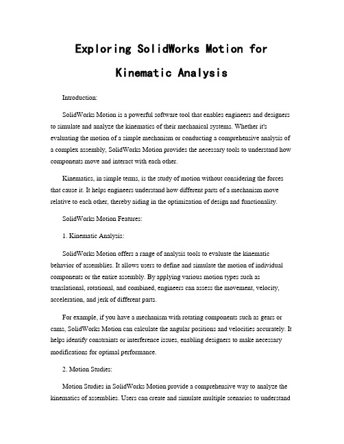
Exploring SolidWorks Motion forKinematic AnalysisIntroduction:SolidWorks Motion is a powerful software tool that enables engineers and designers to simulate and analyze the kinematics of their mechanical systems. Whether it's evaluating the motion of a simple mechanism or conducting a comprehensive analysis of a complex assembly, SolidWorks Motion provides the necessary tools to understand how components move and interact with each other.Kinematics, in simple terms, is the study of motion without considering the forces that cause it. It helps engineers understand how different parts of a mechanism move relative to each other, thereby aiding in the optimization of design and functionality.SolidWorks Motion Features:1. Kinematic Analysis:SolidWorks Motion offers a range of analysis tools to evaluate the kinematic behavior of assemblies. It allows users to define and simulate the motion of individual components or the entire assembly. By applying various motion types such as translational, rotational, and combined, engineers can assess the movement, velocity, acceleration, and jerk of different parts.For example, if you have a mechanism with rotating components such as gears or cams, SolidWorks Motion can calculate the angular positions and velocities accurately. It helps identify constraints or interference issues, enabling designers to make necessary modifications for optimal performance.2. Motion Studies:Motion Studies in SolidWorks Motion provide a comprehensive way to analyze the kinematics of assemblies. Users can create and simulate multiple scenarios to understandhow different design variations affect the motion of a mechanism. By defining relationships, forces, and motion inputs, engineers can observe and compare the behavior of components under various conditions.Motion studies allow for the creation of time-based animations, enabling visualizations of how parts move and interact. This feature is particularly beneficial in communicating design concepts, identifying potential collisions, and validating the functionality of a mechanical system.3. Contact Detection and Collision Analysis:SolidWorks Motion incorporates robust algorithms for detecting and analyzing interferences during the motion simulation of an assembly. This capability helps engineers identify potential collisions or overconstraints that might lead to unintended behavior or failure.By incorporating contact detection and collision analysis, the software allows usersto adjust their designs, modify constraints, or add protective features to prevent collisions. It ensures that your mechanism operates smoothly and safely.4. Motion Optimization:SolidWorks Motion also offers optimization tools to enhance the kinematic performance of designs. This feature enables engineers to set up design parameters and constraints, allowing the software to automatically adjust the design to achieve desired outcomes.By utilizing optimization techniques, users can fine-tune parameters, such as dimensions or constraints, to optimize the efficiency, speed, or accuracy of a mechanism's motion. This leads to cost savings, improved performance, and less iteration during the design process.5. Real-time Analysis:One of the key advantages of SolidWorks Motion is its ability to provide real-time analysis of kinematic behavior. Engineers can observe the motion simulation in real-time, allowing for quick assessments and iterative modifications.The real-time analysis feature enhances the collaboration between design teams as they can share the simulation results during the design review process. It helps in identifying any design or performance issues early on, reducing time and rework.Conclusion:SolidWorks Motion offers a comprehensive set of tools for kinematic analysis, enabling engineers to simulate, analyze, and optimize the motion of mechanical systems. By utilizing these features, designers can gain valuable insights into the behavior of their assemblies, optimize performance, and make informed design decisions.From kinematic analysis to motion studies, contact detection to optimization, and real-time analysis to improve collaboration, SolidWorks Motion provides a powerful platform to explore the kinematics of mechanical systems. By utilizing this software, engineers can enhance the quality, efficiency, and reliability of their designs, leading to improved product performance and customer satisfaction.。
腱绳驱动仿人灵巧手运动分析

NEW PRODUCT NEW TECHNOLOGY0 引言伴随着工业及科技领域的蓬勃发展,中国对航空航天、核工业等战略性产业愈加重视。
在这些工业场景中,工作人员通常需要在极端、危险的条件下进行作业,对人身体健康会产生较大危害。
为此,可替代技术人员进入此类极端工业场景完成复杂工作任务的智能机器人应运而生,其末端执行器的选择直接影响了机器人的工作效率。
作为结合了仿生学新型末端执行器[1,2]的灵巧手,拥有灵巧性高、适应性强、可完成多种不同类型的复杂操作等优点,成为近年来机器人领域研究的热点。
仿人灵巧手可分为全驱动仿人灵巧手和欠驱动仿人灵巧手[3-7]2类。
针对欠驱动灵巧手的发展和研究,美国宇航局(NASA)对在航天领域应用的空间机器人研制了早期最为经典的一种欠驱动灵巧手Robonaut Hand[8],此后又与通用汽车合作对上一代灵巧手进行优化研制了第二代Robonaut Hand。
Catalano M G等[9]研制了PISA/IIT SoftHand,这种手仅用单一舵机驱动整个具有19个自由度的灵巧手,其很好地利用了腱绳驱动方式的优势,为腱绳驱动灵巧手提供了思路。
徐昱琳等[10]研制的SHU-Ⅱ采用轻质腱绳驱动并将6个直流电动机内置于手掌,其中5个电动机分别控制各手指弯曲运动,余下的1个电动机控制拇指侧摆,具有较大的运动抓取空间。
基于此,本文设计了一种腱绳驱动仿人灵巧手,先对其进行运动学分析,再求出其雅克比矩阵,分析手指动力学性能和运动空间,为仿人灵巧手提供控制依据和理论。
1 仿人灵巧手的总体设计本文灵巧手依据人手作为仿生对象,根据人体手部腱绳驱动仿人灵巧手运动分析王峥宇1 张 立1 陈耀轩1 梅 杰1,2 陈定方1,21武汉理工大学交通与物流工程学院 武汉 430063 2武汉理工大学智能制造与控制研究所 武汉 430063摘 要:针对在极端环境下代替人工进行作业的需求,文中设计了一种由腱绳驱动的灵巧手作为高效机器人末端执行器。
kinematic Analysis
3Kinematic AnalysisThe kinematic constraint equations corresponding to the natural coordinates were explained in detail in Chapter 2, both for planar and three-dimensional multibody systems. They were then compared to other types of coordinates. Attention was also given to the main sources of constraint equations with natural coordinates: rigid body constraints, joint constraints, and the optional definition of relative or joint coordinates.In this chapter we will make use of those constraint equations to solve what is usually called kinematic problems, namely, the initial position or assembly problem, the finite displacement problem, and the velocity and acceleration analysis. The first two problems require an iterative solution of a system of nonlinear equations. Some special techniques to improve the convergence will be explained. Special attention will be addressed to the important case of over constrained multibody systems or, in general, to systems with non-independent constraint equations. The last section of this chapter is devoted to the case of non-holonomic joints.3.1 Initial Position ProblemThe initial position problem was defined in Section 1.3. It basically consists of determining the position of all the bodies in the system by knowing the positions of the fixed and the input bodies which can also be called guided or driven ele-ments. Mathematically, the initial position problem is reduced to determining from the known coordinates corresponding to the input elements the vector of dependent coordinates that satisfies the nonlinear system of constraint equa-tions. Note that the input can also be specified as the externally guided or driven linear or angular coordinates corresponding to several joints (as many joints as there are degrees of freedom) on which mixed coordinates have been defined. This basic notion is explained by means of the following examples:7172 3. Kinematic AnalysisFigure 3.1. Four-bar mechanism modeledwith natural coordinates.Figure 3.2. Four-bar mechanism modeled with mixed coordinates.Example 3.1As a first example, the four-bar mechanism of Figure 3.1 will be considered. This sys-tem has four natural coordinates (x 1,y 1,x 2,y 2).The constraint equations corresponding to this mechanism are following constant distance conditions:x 1 Ð x A 2 + y 1 Ð y A 2 Ð L 22 =02 Ð x 12 + y 2Ð y Ð L 32 = 0x 2 Ð x B 2 + y 2 Ð y B 2 Ð L 42 = 0These three equations are not sufficient to determine the four unknown variables of the problem. In fact, it is still necessary to enter the condition that the position of the input element (element 2) is known. If both coordinates of point 1 are known, then only two unknown variables are left. In this case, it is obvious that the first constraint equation which establishes the constant length condition of element 2 no longer makes any sense, because it does not contain any unknown variable. Consequently the prob-lem reduces to the finding of x 2 and y 2, using the last two nonlinear quadratic con-straint conditions.Example 3.2Let us consider the four-bar mechanism shown in Figure 3.2, which uses mixed coor-dinates; that is, the same coordinates as in example 3.1 plus the angle y between ele-ments 2 and 3 at joint 1. Let's assume that, instead of the position of the input element,one knows the angle y . In this case the constraint equations will be as follows (assuming a suitable value for y to be able to use the scalar product):x 1 Ð x A 2 + y 1 Ð y A 2 Ð L 22 = 02 Ð x 12 + y 2 Ð y Ð L 32 = 0x 2 Ð x B 2 + y 2 Ð y B 2 Ð L 42 = 0x 1 Ð x A 2 Ð x 1 +1 Ð y y 2 Ð y Ð L 2 L 3 cos y = 03.1 Initial Position Problem 73Figure 3.3. RSCR mechanism modeled with natural coordinates.which is a system with four equations and four unknown variables, assuming that the externally driven angle y is known.Example 3.3Figure 3.3 depicts a three-dimensional four-bar mechanism RSCR (Revolute-Spherical-Cylindrical-Revolute) modeled with natural coordinates. This mechanism has three movable points and one movable unit vector; that is, twelve dependent Cartesian coordinates and one degree of freedom. Also the input angle y has been in-troduced as an additional externally driven coordinate. The constraint equations corre-sponding to this mechanism are the following:1. 1 Ð x 0 Ð x y 1 Ð y A y 0 Ð y A 1 Ð z 0 Ð z k 1 cos y = 02.1 Ð x 1 Ð y 1 Ð z Ð k2 = 03.1 Ð x Ax 1 Ð y Ay 1 Ð z Az Ð k 3 = 04.x 2 Ð x 2 Ð y 12 + z 2 Ð z Ð k 4 = 05.x 2 Ð x 1x + y 2 Ð y 1y + z 2 Ð z 1z Ð k 5 = 0 6.u 1x 2 + u 1y 2 + u 1z 2 Ð 1= 07.x 3 - x B + y 3 - y B + z 3 - z B Ð k 6 = 08.x 3 Ð x B u 1x 3 Ð y 1y + z 3 Ð z B u 1z Ð k 7 = 09.x 3 Ð x B u Bx + y 3 Ð y B u By + z 3 Ð z B u Bz Ð k 8 = 010.u Bx u 1x + u B y u 1y + u B z u 1z Ð k 9 = 011.y 3 Ð y 1z 3 Ð z 2 u 1y = 012.z 3 Ð z 1x Ð x 3 Ð x 1z = 013.x 3 Ð x 1y Ð y 3 Ð y 1x = 0This is the system of nonlinear equations that governs the position problem for the RSCR mechanism. The first equation corresponds to the input angle definition; equa-74 3. Kinematic Analysistions 2 and 3 represent rigid body condition for element 2; equations 4 to 6 represent rigid body constraints for element 3; equations 6 to 10 represent the same for element 4, and equations 11 to 13 (only two of them are independent) contribute to define the cylindrical joint. Finally, k i (i=1,...,9) represents constant values.The above examples clearly indicate that irrespective of the multibody sys-tems being considered, the position problem is always based on solving the con-straint equations, which make up the following set of equations:F(q, t)=0(3.1) where q is the vector of the system dependent coordinates. It will be assumed that there are at least as many equations as there are unknown variables or coor-dinates. To solve systems of nonlinear equations such as (3.1), it is customary to resort to the well-known Newton-Raphson method which has quadratic conver-gence in the neighborhood of the solution (the error in each iteration is propor-tional to the square of the error in the previous iteration) and does not usually cause serious difficulties if one starts with a good initial approximation.The Newton-Raphson method is based on a linearization of the system (3.1) and consists in replacing this system of equations with the first two terms of itsexpansion in a Taylor series around a certain approximation qi to the desiredsolution. Once the substitution has been made, the system (3.1) becomesF(q, t)@F(q i)+F q(q i)(q Ð q i)=0(3.2) where the time variable has not been accounted for, so that in this problem has a constant value. Matrix F q is the Jacobian matrix for constraint equations; that is to say, the matrix of partial derivatives of these equations with respect to the de-pendent coordinates. This matrix takes the following form:F q=¶f1¶q1¶f1¶q2.......¶f1¶q n¶f2¶q1¶f2¶q2.......¶f2¶q n ...................¶f m¶q1¶f m¶q2.......¶f m¶q n(3.3)In equation (3.3), m is the number of constraint equations and n the number of dependent coordinates. If the constraint equations are independent, f=n-m is the number of degrees of freedom of the multibody system.Equation (3.2) represents a system of linear equations constituting an approx-imation to the nonlinear system (3.1). The vector q, obtained from the solution of equation (3.2), will be an approximation of the solution in (3.1). By calling this approximate solution qi+1, a recursive formula is obtained as follows:F(q i)+F q(q i)(q i+1Ð q i)=0(3.4)3.1 Initial Position Problem 75qFigure 3.4. Iteration process of the Newton-Raphson method.which can be used repeatedly until the error in the system of equations (3.1) is insignificant, or until the difference between the results of two successive itera-tions is smaller than a pre-specified tolerance. Figure 3.4 shows the geometric representation of the Newton-Raphson method for the case of a nonlinear equa-tion with one unknown. The function F(q) is linearized at point qi , i.e. substi-tuted by its tangent linear space, which are the first two terms of the Taylor ex-pansion formula. The point where the tangent space intersects the horizontal axisis the approximate solution qi+1. The function F(q) is again replaced at pointq i+1by the new tangent space and a new approximate solution qi+2is found. Onearrives ultimately within the desired accuracy to the exact solution q.Note that the Newton-Raphson iteration will not always converge to a solu-tion. It has been pointed out that if the initial approximation is not close enough to a solution, the algorithm may diverge. There is still another source of difficul-ties. If the values of the input variables do not correspond to a possible physical solution, the mathematical algorithm will fail irrespective of how the initial ap-proximation has been chosen.The Jacobian matrix of the constraint equations, defined by means of equa-tion (3.3), plays an extremely important role in all kinematic and dynamic analy-sis problems. In the equation (3.4), the Jacobian matrix determines the linear equation system used to find the successive approximations for solving the ini-tial position problem. Evaluating and triangularizing this matrix easily and quickly are characteristics of all good multibody system analysis methods. The natural coordinates permit the performance of these operations in the best possible way.In Section 1.2, it was stated that the initial position problem had multiple so-lutions, and this is indeed the case. Depending on the vector qo where the itera-tion begins, some solution will be attained.Example 3.4To complete this section on the initial position problem, the equations (3.4) corre-sponding to the four-bar mechanism studied in Examples 3.1 and 3.2 will be com-76 3. Kinematic Analysisa)b)Figure 3.5. Iteration process of the Newton-Raphson method in a four-bar mechanism.pletely developed. The constraint equations of this case were presented in Example3.1, and consequently the equation (3.4) takes the following form:2x1Ðx A y1Ðy A00x1Ðx2y1Ðy2x2Ðx1y2Ðy100x2Ðx B y2Ðy B ix1y1x2y2i+1Ðx1y1x2y2i==Ðx1Ðx+1ÐyÐL22x2Ðx+2Ðy12ÐL32x2Ðx+2ÐyÐL42iIn this system of equations, at least one of the four unknown coordinates must be known ahead of time in order to be able to solve the problem. If, for example, x1 is known, then:(x1)i+1 Ð (x1)i = 0and the first column of the Jacobian matrix is multiplied by zero, meaning that it can be eliminated.In the case of the four-bar mechanism of Figure 3.2, modeled with mixed coordi-nates and whose constraint equations are presented in Example 3.2, equation (3.4) be-comes:2(x1Ð x A)2(y1Ð y A)0002(x1Ð x2)2(y1Ð y2)2(x2Ð x1)2(y2Ð y1)0002(x2Ð x B)2(y2Ð y B)0 (x2Ðx1+x AÐx1)(y2Ðy1+y AÐy1)(x1Ð x A)(y1Ð y A)(L2 L3 sin y)i..x1y1x2y2y i+1Ðx1y1x2y2y i=(x1Ðx A)2+(y1Ðy A)2Ð L22(x2Ðx1)2+(y2Ðy1)2Ð L32(x2Ðx B)2+(y2Ðy B)2Ð L42(x1Ðx A)(x2Ðx1)+(y1Ðy A)(y2Ðy1)Ð L2 L3 cos y i3.1 Initial Position Problem 77Figure 3.6. Possible divergence in the Newton-Raphson iterationUsually, the angle y is known; therefore, the last unknown variable (y i+1 Ð y i ) has a zero value. Thus the fifth column of the Jacobian matrix can be eliminated.One characteristic common to the Jacobians matrices shown in this example (and in all the Jacobians matrices calculated with natural coordinates) is that they are linear functions of the dependent variables. For example, Figures 3.5a and 3.5b include drawings of the initial approximation, the first iterations, and the final solution of the initial position problem in the two four-bar mechanisms of Figures 3.1 and 3.2 com-puted according to the above expressions.The Newton-Raphson method, explained in this section, converges rather quickly (quadratic convergence) when it is close to the desired solution. At times, and during the first iterations, it can give very abrupt jumps as a result of not having started from a sufficiently good initial approximation. Figure 3.6shows what could happen in this case. The approximate solution q i+1 is further away from the true solution q , than the previous approximation q i . It is even possible that the value of function F (q ), a function that should be equal to zero,could increase when moving from q i to q i+1.This problem is not easy to solve without resorting to much more compli-cated numerical methods. In general, one should do everything possible to start from good initial approximations. If this cannot be achieved, then one should try to apply a reduction to the coordinates modification given by equation (3.4) and to apply it to the previous approximate solution q i . As this often works, a cor-rection factor of 1/2 or 1/3 is recommended. Finally, one should always make sure that the module of F (q ) decreases when going from point q i to q i+1.Some authors have solved the position problem at times by calculating differ-ent solutions numerically by means of the so-called continuation methods (Tsai and Morgan (1985)). Continuation methods start out from a position where the multibody system complies with all the constraint equations, although the input elements might not be at the desired position and the fixed joints might not be at78 3. Kinematic Analysistheir final position. With relaxed conditions regarding the input elements and the fixed element, it is not difficult to find a position on the multibody system that satisfies the constraint equations. Then, by means of small finite displacements whose convergence is guaranteed by the Newton-Raphson method, an attempt is made to move the input elements and the fixed joints to their correct position. At times, the bifurcation points (points at which two or more possible movements can occur) provide a way of finding different solutions to the position problem.3.2 Velocity and Acceleration Analysis3.2.1 Velocity AnalysisThe equations that permit solving the velocity problem originate after one dif-ferentiates with respect to time the constraint equations. If these equations are represented symbolically asF (q , t ) = 0(3.5)by differentiating with respect to time, the following equation is obtained:F ,q =ÐF t ºb (3.6)where F q is the Jacobian matrix defined by means of equation (3.3). Vector q is the vector of dependent velocities (derivative with respect to the time of the vec-tor of dependent coordinates or position variables). Vector (ÐF t = b ) is the par-tial derivative of the constraint equations with respect to time. If all the con-straints are scleronomous, meaning that there are no rheonomous or time depen-dent constraints, this derivative will be zero) If the position of the multibody system is known, equation (3.6) allows us to determine the velocities of the multibody system by starting from the velocity of the input elements. Just as in the position problem, the matrix that controls the velocity problem is the Jacobian matrix of the constraint equations. The essential difference between both problems is that where the position problem is nonlinear, the equations governing the velocity problem are linear. This means that the equations do not have to be iterated, and there is only one solution to a properly posed problem.The following example illustrates these concepts:Example 3.5As an example of this, the velocity equations of the four-bar mechanism of Figure 3.1will be determined below by using: a) relative coordinates, b) reference point coordi-nates, c) natural coordinates, and d) mixed coordinates.a)Using relative coordinates , the constraint equations are given by (See Section2.1.1),L 1 cos Y 1 + L 2 cos (Y 1 + Y 2) + L 3 cos (Y 1 + Y 2 + Y 3) Ð O D = 03.2 Velocity and Acceleration Analysis 79L1 sin Y1+ L2 sin (Y1+Y2)+ L3 sin (Y1+Y2+Y3)=0Differentiating these equations with respect to time, we obtain:ÐL1 sin y1y1Ð L2 sin (y1+y2)(y1+y2)ÐÐ L3 sin (y1+y2+y3)(y1+y2+y3)=0L1 cos y1y1+ L2 cos (y1+y2)(y1+y2)++ L3 cos (y1+y2+y3)(y1+y2+y3)=0and by rearranging these equations, we arrive at:Ð L1s1Ð L2s12Ð L3s123Ð L2s12Ð L3s123Ð L3s123 L1c1+ L2c12+ L3c123 L2c12+ L3c123 L3c123y1 y2 y3where s1 = sin y1, s12 = sin (y1 + y2), and so forth.If one of the three velocities in the previous equation is known such as the one cor-responding to the input coordinate) the corresponding column of the Jacobian matrix can be moved to the right-hand side of the equation. This results in a system of two linear equations with two unknown velocities that can be solved with no difficulties.b)Using reference point coordinates,the constraint equations are represented by (SeeSection 2.1.2):x1ÐxÐL12 cos Y1=y1ÐyÐL12 sinY1=02Ðx1ÐL12 cos Y1Ð L22 cos Y2=y2ÐyÐL12 sin Y1Ð L22 sinY2=03Ðx2ÐL22 cos Y2Ð L32 cos Y3=y3ÐyÐL22 sin Y2Ð L32 sin Y3=0x3Ðx DÐL32 cos Y3=0y3Ðy DÐL32 sin Y3=0and the time derivatives are:x1+ L1/2Y1 sin Y1=0y1Ð L1/2Y1 cos Y1=0x2Ð x1+L12Y1 sin Y1+L22Y2 sin Y2=0y2Ð y1ÐL12Y1 cos Y1ÐL22Y2 cos Y2=0x3Ð x2+L22Y2 sin Y2+L32Y3 sin Y3=0y3Ð y2ÐL22Y2 cos Y2ÐL32Y3 cos Y3=0x3+L32y3 sin Y3=0y3ÐL32Y3 cos Y3=080 3. Kinematic AnalysisThese equations can be expressed in matrix form as follows:F q q =0where the matrix F q is10s1L1/200000001Ðc1L1/2000000Ð10s1L1/210s2L2/20000Ð1Ðc1L1/201Ðc2L2/2000000Ð10s2L2/210s3L3/20000Ð1Ðc2L2/201Ðc3L3/200000010s3L3/200000001Ðc3L3/2 which is a system of eight equations with nine unknown velocities. If the angular ve-locity y1 is known for element 2, the third column of the Jacobian matrix will be moved to the right side member. The result will be a system of eight linear equations with eight unknown velocities.c)With natural coordinates the constraint equations (Section 2.1.3) are representedby:(x1Ð x A)2+(y1Ð y A)2Ð L22=0(x2Ð x1)2+(y2Ð y1)2Ð L32=0(x3Ð x B)2+(y3Ð y B)2Ð L42=0whose time derivatives are:(x1Ð x A) x1+(y1Ð y A) y1=0(x2Ð x1)(x2Ð x1)+(y2Ð y1)(y2Ð y1)=0(x2Ð x B) x2+(y2Ð y B) y2=0and in matrix form yields:(x1Ðx A)(y1Ðy A)00 (x1Ðx2)(y1Ðy2)(x2Ðx1)(y2Ðy1) 00(x2Ðx B)(y2Ðy B)x1 y1 x2 y2By knowing one of the four natural velocities and by moving the corresponding column to the right-hand side of this equation, one can find the remaining velocities with the resulting set of three linear equations and three unknown variables.d)Using mixed coordinates, the constraint equations (Section 2.1.4) are:(x1Ð x A)2+(y1Ð y A)2Ð L22=0(x2Ð x1)2+(y2Ð y1)2Ð L32=0(x3Ð x B)2+(y3Ð y B)2Ð L42=0(x1Ð x A)(x2Ð x1)+(y1Ð y A)(y2Ð y1)Ð L2 L3 cos Y=03.2 Velocity and Acceleration Analysis 81Figure 3.7. Results of a velocity analysis in a four-bar mechanism.differentiating with respect to time:x1Ðx A x1+y1Ðy A y1=0x2Ðx x2Ðx+y2Ðy y2Ðy=0x2Ðx B x2+y2Ðy B y2=02Ðx1 x1+x1Ðx AÐx1+2Ðy1 y1++y1Ðy A y2Ðy1+L2L3 sin y y=0which can be expressed in matrix form as1Ðx1Ðy0001Ðx21Ðy22Ðx12Ðy10002Ðx2Ðy0x2Ð2x1+x A y2Ð2y1+y A1Ðx1Ðy L2L3sin yx1y1x2y2y=If y is known, the fifth column will be moved to the right-hand side and will leave four equations with four unknowns. Figure 3.7 shows the result of a velocity analysis in accordance with an input velocity of y =1.3.2.2 Acceleration AnalysisThe finding of the dependent acceleration vector q becomes apparent by simply differentiating with respect to time the velocity equation (3.6). This yields the following result:F q,q=ÐtÐq q º c(3.7)If the position vector q and the velocity vector q are known, by solving the system of linear equations (3.7), one can find the dependent acceleration vector q. Note that the leading matrix of the systems of linear equations (3.6) and (3.7) is exactly the same. As a consequence, if it has been formed and triangularized82 3. Kinematic AnalysisFigure 3.8. Results of an acceleration analysis in a four-bar mechanism.to solve the velocity problem, the acceleration analysis can be carried out by simply forming the right-hand side and by performing a forward reduction and backward substitution. When there are no rheonomous or time-dependent con-straints, the velocity problem is homogeneous; whereas the acceleration problem is always non-homogeneous as long as the velocities are not equal to zero.Equation (3.7) can be differentiated once again to obtain the jerk or over ac-celeration equation:F q d dt = Ð t Ð 2 q q Ð q q (3.8)Once again a system of linear equations has been obtained whose leadingmatrix is the Jacobian matrix of the constraint equations.Example 3.6Included below are the acceleration equations for the four-bar mechanism of Example3.5d modeled with mixed coordinates. These equations are obtained by differentiating the corresponding velocity equations:1Ðx 1Ðy 0001Ðx 21Ðy 22Ðx 12Ðy 10002Ðx 2Ðy 0x 2Ð2x 1+x A y 2Ð2y 1+y A1Ðx 1Ðy L 2 L 3 sin y = Ð x 1y 1000x 1Ðx y 1Ðy x 2Ðx y 2Ðy 000x 2y 20x 2Ð2x 1y 2Ð21x 1y 1L 2 L 3 cos y x 1y 1x 2y 2y3.2 Velocity and Acceleration Analysis 83If all the velocities q and input accelerations y are known, the remaining accelera-tions q can be calculated by means of the four equations with four unknowns resulting from moving the fifth column, multiplied by y, to the RHS of the acceleration equa-tion. Figure 3.8 graphically shows the result of an acceleration analysis that corre-sponds to the expression developed in this example.3.3 Finite Displacement AnalysisThe finite displacement analysis is closely related to the initial position problem, and is controlled by the same system of nonlinear equations (the kinematic constraint equations). The velocity and acceleration analyses are used at times in finite displacement analysis to improve the initial approximation with which the iterative process begin, which explains the reason for including it here and not immediately after the initial position problem.3.3.1 Newton-Raphson IterationAs explained in Section 1.2, once one knows a position of the multibody system where all the constraint equations are satisfied, the finite displacement problem consists of finding the new position that the system takes when a finite displace-ment is applied to each one of the input elements or externally driven relative coordinates. Finite displacement is understood to be any movement other than infinitesimal.The main problem dealt with in this section is of the same nature and conse-quently controlled by the same equations of the position problem. Therefore, the Newton-Raphson method can be used for solving it. The difference between both problems lies in the fact that the finite displacement problem usually relies on a good initial approximation which is obtained from a previous exact posi-tion where all the elements satisfy the constraints. It is possible to improve upon the approximation by means of a velocity and acceleration analysis, as will be described in the next section.These advantages do away with many of the convergence problems encoun-tered in the initial position problem. In addition, the problem of multiple solu-tions becomes marginal. If the displacement of the input elements is small enough, then of all the possible solutions for the constraint equations, the correct one will be the closest to the starting position. This is precisely the one obtained by the Newton-Raphson iterations. However, there still remains the possibility of driving or trying to drive the multibody system to unfeasible positions, that is, positions that cannot be reached without violating some constraints equations. Trying to move the end-effector of a robot out of its workspace is an example of a finite displacement problem where the Newton-Raphson method will necessar-ily fail to find a correct solution.84 3. Kinematic AnalysisBFigure 3.9. Improving the initial approximation.A2' BFigure 3.10. Better estimate for an initial approximation.3.3.2 Improved Initial ApproximationIn order to determine and improve the initial or starting approximation, the ex-ample of the four-bar mechanism will be used once again. This will clearly de-scribe the method without any loss of generality.Figure 3.9 shows a four-bar mechanism, in which the input element has been rotated a finite angle. One possible way of generating an initial approximation is by not varying the remaining natural coordinates as in the starting position shown in Figure 3.9. This approximation leads to a severe violation of the con-straint equations.The initial approximation shown in Figure 3.9 can be improved upon by means of velocity analysis, as indicated in Figure 3.10. The velocity analysis is carried out by imposing a velocity at the input element so that the endpoint 1' of the velocity vector of 1 is the closest point to 1" over the perpendicular to A-1 (1'-1" is parallel to A-1).3.3 Finite Displacement Analysis 85Since 1" is known, it is not difficult to determine the velocity of the input el-ement such that the end of the velocity vector at point 1 is 1'. Using this velocity as input, a velocity analysis is performed, and the ends of the velocity vectors are determined for all the basic points of the mechanism (in Figure 3.10, 2' is the end of the velocity vector of point 2).The initial approximation used to start the iterations for the Newton-Raphson method is indicated by the dotted lines in Figure 3.10 It is an improvement over the one in Figure 3.9. Note that the initial approximation is (A-1"-2'-B) and not (A-1'-2'-B). The exact position 1" of point 1 is known because it belongs to the input element and this exact position should be used.It is not essential that point 1' be the closest one to 1" on the tangent to the trajectory of 1. Another simpler possibility for calculating point 1' and the velocity of the input element, is to assume that point 1 changes to position 1" in an arbitrary period of time such as 1 second. Next, calculate the angular velocity of the input element by dividing angle 1-1" (in radians) by the said amount of time where the quotient is the said angular velocity. The position at the initial approximation of any point P can be calculated by means of the following expression:q = q o + q D t (3.9) Equation (3.9) is an approximate integral of velocities starting from the previ-ous position. An approximate integration which also causes the accelerations to intervene can be obtained in a similar manner:q D t2(3.10)q = q o + q D t + 12This formula suggests that the initial approximation can be constructed start-ing from a velocity analysis and an acceleration analysis. To calculate the veloc-ity and acceleration of the input element one may proceed as follows:1.Apply one of the previously studied methods and determine the velocity ofthe input elements.2.Knowing the initial and final position of the input elements and their veloc-ity, determine the acceleration to be applied to them applying equation (3.10) to the input elementsDetermination of the initial approximation by means of velocity and accelera-tion analysis allows the iterations to begin with a better approximation to the fi-nal solution. The cost of an acceleration analysis is small if a velocity analysis has already been performed. The matrix for both systems of equations is the same, and one only needs to form it and triangularize it once. Based on the expe-rience gained through numerical experiments performed by the authors, the ini-tial approximation constructed with velocities and accelerations does not always give better results than the one determined from velocities only.。
asymptotic analysis缩写
asymptotic analysis缩写
Asymptotic Analysis 的意思是 "极限分析",指的是在算法或
数学模型中,当样本数量趋近于无穷大时,所计算的结果或估计值趋
向于某个确定的极限值,通常称为无穷大极限或无穷级数。
这种分析方法常用于对连续函数、概率分布等进行分析和估计。
例如,在数学中,当函数 $f(x)$ 在 $x=a$ 处取得极小值时,可
以通过引入 $a$ 的无穷大来估计 $f(x)$ 的值。
这个估计值可以表示为 $f(a) approx lim_{x to a^-} f(x)$。
其中,$lim_{x to a^-} f(x)$ 表示当 $x$ 趋近于 $a$ 时,$f(x)$ 的值趋近于某个值,这个值称为极限值。
Asymptotic Analysis 是一种重要的数学分析方法,可以帮助研究者更好地理解并预测复杂系统的性能和行为,尤其是在当样本数量趋近于无穷大时,系统的行为可能会表现出非常惊人的规律和特性。
往复泵曲柄滑块机构的运动学分析
往复泵曲柄滑块机构的运动学分析付子豪,翟国栋(中国矿业大学(北京)机电与信息工程学院,北京100083)摘要:基于往复式泵的结构及工作原理,文中用解析法对往复泵中的曲柄滑块机构滑块的运动规律进行了分析与讨论,其中对滑块的速度和加速度进行了定量表征,并建立了曲柄滑块的运动本构方程。
对于曲柄的特定位置,以C语言程序编 程对滑块的相关特征参数进行了计算。
这些结果表明:文中探索的曲柄滑块机构运动学分析研究方法具有计算精度高、分 析方便、通用性强的特点。
因此,该研究对实际曲柄滑块机构的逆向设计具有重要的参考价值和指导意义。
关键词:往复式抽水泵;曲柄滑块;运动分析中图分类号:TH 133 文献标志码:A文章编号:1002-2333(2016)12-0119-04 Kinematics Analysis on the Crank Slider of Reciprocating PumpFU Zihao,ZHAI Guodong(School of Electrical and Information Engineering, China University of Mining and Technology (Beijing), Beijing 100083, China) Abstract:Based on the structural characterizations and working principle of reciprocating pump, the analytical method is used to analyze the slider motion low of crank -slider mechanism in reciprocating pump, in which the velocity and acceleration of the slider are quantitatively characterized. This paper establishes the constitutive equation of motion of slider crank mechanism. For the specific position of the crank, the related characteristic parameters of the sliding block are calculated using the C programming language program. These results indicate that this method has the advantages of high accuracy, simple and strong commonality. Therefore, this study has important reference value and guiding significance for the design of the actual crank slider mechanism.Key words:reciprocating pump; crank slider; kinematic analysis0引言在往复式泵的结构设计中,往往需要对其主体机构曲柄滑块机构进行运动学及强度分析,并且根据运动学分析结果建立起相应的数学模型。
1-D KINEMATICS - LESSON 1(加拿大高中物理第一课)
goal should be to become very familiar with their meaning. You may
click on any word now to
Kinematics is the science of describing the motion of objects using words, diagrams, numbers, graphs, and euations. Kinematics is a branch of mechanics. The goal of any study of kinematics is to develop sophisticated mental models which serve to describe (and ultimately, explain) the motion of real-world objects.
investigation into the physics of motion. As we focus on the language, principles, and laws which describe and explain the motion of objects, your efforts should center around internalizing the meaning of the information. Avoid memorizing the information; and avoid abstracting the information from the physical world which it describes and explains. Rather, contemplate the information, thinking about its meaning and its applications.
- 1、下载文档前请自行甄别文档内容的完整性,平台不提供额外的编辑、内容补充、找答案等附加服务。
- 2、"仅部分预览"的文档,不可在线预览部分如存在完整性等问题,可反馈申请退款(可完整预览的文档不适用该条件!)。
- 3、如文档侵犯您的权益,请联系客服反馈,我们会尽快为您处理(人工客服工作时间:9:00-18:30)。
ε
θ
In TRUE BASIC, formula(公式) XB=XA+L * cos() corresponds to: XB=XA+L*COS (Q) Similarly, formula (VB)X= (VA)X -L*sin()* corresponds to VBX=VAX-L*SIN(Q)*W Formula (aB)X=(aA)X-L*sin()*-L*cos()* 2 corresponds to ABX=AAX-L*SIN(Q)*E-L*COS(Q)* W^2
3.3. Kinematic Analysis by Analytical(解析的) Methods (1) In graphical(图解的) methods, it is very tedious(冗长乏味的) if a mechanism is to be analyzed for a complete cycle. Furthermore, the accuracy(精度) is limited. (2) The analytical solution can be evaluated(求值) on a computer for different dimensions and/or at different positions with very little effort. The accuracy of the solution far surpasses(超越) that required for mechanical design problems.
ε
θ
In a Cartesian co-ordinate system(直角坐标系), ω XB=XA+L* cos(), L YB=YA+L* sin() Differentiating(求导) the above formulae(公式) with respect to time, (VB)X=(VA)X-L*sin()* (VB)Y=(VA)Y+L*cos()* Differentiating again, (aB)X=(aA)X-L*sin()*-L*cos()* 2 (aB)Y=(aA)Y+L*cos()*-L*sin()* 2
E C B A A grade II D F grade III B C C E A
g
Then the kinematic analysis of a multi-bar(多 杆) linkage mechanism is reduced(简化) into two simple steps: (1)First, dividing the mechanism into Assur groups. (2)Secondly, calling(调用) the corresponding(相应的) subroutine for each Assur group according to the type and the assembly(装配) order of the Assur group.
• After the subroutine is called, (XB, YB, VBX, VBY, ABX, ABY)will be known.
3.3.2 The RRR Subroutine In the RRR group, XA , YA , (VA)X , (VA)Y , (aA)X , (aA)Y , XC , YC , (VC)X , (VC)Y , (aC)X , (aC)Y , LAB , and LCB are known. AB , AB , AB , CB , CB , CB are C to be calculated.
ε ω
L
θ
• Any subroutine must begin with statement SUB subroutine-name(table of parameters) and end with statement cilitate(使便利) the understanding of the program, parameters should have easily-recognized(认识) names. • Before the subroutine is called, (XA, YA, VAX, VAY, AAX, AAY, Q, W, E, L)are known.
Advantages of group method: Assur groups have kinematic determination. One can set up subroutines(子程序) in advance(预先) for some commonly used Assur groups.
SUB LINK(XA, YA, VAX, VAY, AAX, AAY, Q, W, E, L, XB, YB, VBX, VBY, ABX, ABY) XB=XA+L*COS(Q) YB=YA+L*SIN(Q) VBX=VAX-L*SIN(Q)*W VBY=VAY+L*COS(Q)*W ABX=AAX-L*SIN(Q)*E-L*COS(Q)*W^2 ABY=AAY+L*COS(Q)*E-L*SIN(Q)*W^2 END SUB
3.3.1 The LINK Subroutine Suppose that the X and Y components(分 量) of position, velocity, and acceleration of a point A (i.e. XA, YA, (VA)X, (VA)Y, (aA)X, (aA)Y), the angular position, the angular velocity, and the angular acceleration of link AB(i.e. , , ), and the length (L) of the link AB are known. XB, YB, (VB)X, (VB)Y, (aB)X, (aB)Y are to be calculated. ω L