损伤层合板壳非线性分析(傅衣铭著)思维导图
复合材料层合板渐进损伤分析与试验验证
复合材料层合板渐进损伤分析与试验验证作者:曾昭炜等来源:《无线互联科技》2015年第03期摘要:文章基于能量耗散的渐进损伤分析方法,建立了复合材料层合板的三维有限元模型。
采用了带剪切非线性的修正三维Hashin准则作为单元失效判据,使用Linde模型对失效单元进行材料性能退化。
通过编写用户自定义材料子程序(UMAT),实现了失效准则与材料退化准则在Abaqus中的应用。
并通过试验对有限元模型进行了验证,仿真误差为7.8%。
仿真分析得到的失效位置与失效模式和试验一致,表明文章模型能合理有效地进行层合板的强度预测和失效分析。
关键词:复合材料层合板;渐进损伤分析;UMAT;试验近年来,复合材料以其较高的比强度、比模量,较强的抗疲劳能力、抗振能力和可设计性等特点,在新一代飞机机体结构中得到越来越重要而广泛的应用[1]。
据统计,在飞机结构中,复合材料从空客A380上25%[2]的用量,到波音787的50%,再到A350的52%,其应用增长已经达到年均9%的水平[3]。
另一方面,尽管复合材料正朝着整体化设计加工方向发展,某些部位如维护口盖、机械连接等位置,不得不在复合材料结构上开孔。
相对于金属材料,复合材料层合板开孔部位应力分布更为复杂、应力集中更为严重。
又由于在失效破坏模式方面复合材料结构更为多样复杂,其极限强度分析也十分困难。
因此,研究复合材料结构开孔处性能具有重要的工程意义。
对于开孔层合板的分析研究,主要有孔边应力法、两参数法、临界单元法和渐进损伤分析方法,在开孔层合板压缩强度的分析计算上前三种方法都能够适用,然而由于没有考虑其多种失效模式,在计算精度方面需要得到提高[4]。
渐进损伤分析方法可用于含孔层合板在拉伸载荷作用下内裂纹扩展情况的分析,能够更为有效地对复合材料进行损伤模拟和强度预测。
另外,该方法还能够准确研究复合材料失效模式和失效位置。
1 渐进损伤分析作为渐进损伤分析方法,其基本假设为结构中的材料产生损伤后材料的力学性能将发生一定程度退化,但同时能够继续承载,在此基础上对结构的失效进行分析计算。
Principles of Plasma Discharges and Materials Processing第3章
CHAPTER3ATOMIC COLLISIONS3.1BASIC CONCEPTSWhen two particles collide,various phenomena may occur.As examples,one or both particles may change their momentum or their energy,neutral particles can become ionized,and ionized particles can become neutral.We introduce the funda-mentals of collisions between electrons,positive ions,and gas atoms in this chapter, concentrating on simple classical estimates of the important processes in noble gas discharges such as argon.For electrons colliding with atoms,the main processes are elastic scattering in which primarily the electron momentum is changed,and inelas-tic processes such as excitation and ionization.For ions colliding with atoms,the main processes are elastic scattering in which momentum and energy are exchanged, and resonant charge transfer.Other important processes occur in molecular gases. These include dissociation,dissociative recombination,processes involving negative ions,such as attachment,detachment,and positive–negative ion charge transfer,and processes involving excitation of molecular vibrations and rotations. We defer consideration of collisions in molecular gases to Chapter8.Elastic and Inelastic CollisionsCollisions conserve momentum and energy:the total momentum and energy of the colliding particles after collision are equal to that before collision.Electrons and fully stripped ions possess only kinetic energy.Atoms and partially stripped ions have internal energy level structures and can be excited,de-excited,or ionized, Principles of Plasma Discharges and Materials Processing,by M.A.Lieberman and A.J.Lichtenberg. ISBN0-471-72001-1Copyright#2005John Wiley&Sons,Inc.43corresponding to changes in potential energy.It is the total energy,which is the sum of the kinetic and potential energy,that is conserved in a collision.If the internal energies of the collision partners do not change,then the sum of kinetic energies is conserved and the collision is said to be elastic.Although the total kinetic energy is conserved,kinetic energy is generally exchanged between particles.If the sum of kinetic energies is not conserved,then the collision is inelas-tic.Most inelastic collisions involve excitation or ionization,such that the sumof kinetic energies after collision is less than that before collision.However,super-elastic collisions can occur in which an excited atom can be de-excited by acollision,increasing the sum of kinetic energies.Collision ParametersThe fundamental quantity that characterizes a collision is its cross section s(v R), where v R is the relative velocity between the particles before collision.To define this,we considerfirst the simplest situation shown in Figure3.1,in which aflux G¼n v of particles having mass m,density n,andfixed velocity v is incident on a half-space x.0of stationary,infinitely massive“target”particles having density n g.In this case,v R¼v.Let d n be the number of incident particles per unit volume at x that undergo an“interaction”with the target particles within a differential distanced x,removing them from the incident beam.Clearly,d n is proportional to n,n g,and d x for infrequent collisions within d x.Hence we can writed n¼Às nn g d x(3:1:1)where the constant of proportionality s that has been introduced has units of area and is called the cross section for the interaction.The minus sign denotes removal from the beam.To define a cross section,the“interaction”must be specified,for example,ionization of the target particle,excitation of the incident particle to a given energy state,or scattering of the incident particle by an angle exceeding p=2.Multiplying(3.1.1)by v,wefind a similar equation for theflux:d G¼Às G n g d x(3:1:2) FIGURE3.1.Aflux of incident particles collides with a population of target particles in the half-space x.0.44ATOMIC COLLISIONSFor a simple interpretation of s,let the incident and target particles be hard elastic spheres of radii a1and a2,and let the“interaction”be a collision between the spheres.In a distance d x there are n g d x targets within a unit area perpendicular to x.Draw a circle of radius a12¼a1þa2in the x¼const plane about each target.A collision occurs if the centers of the incident and target particles fall within this radius.Hence the fraction of the unit area for which a collision occurs is n g d x p a212.The fraction of incident particles that collide within d x is thend G G ¼d nn¼Àn g s d x(3:1:3)wheres¼p a212(3:1:4)is the hard sphere cross section.In this particular case,s is independent of v.Equation(3.1.2)is readily integrated to give the collidedfluxG(x)¼G0(1ÀeÀx=l)(3:1:5) with the uncollidedflux G0eÀx=l.The quantityl¼1n g s(3:1:6)is the mean free path or the decay of the beam,that is,the distance over which the uncollidedflux decreases to1=e of its initial value G0at x¼0.If the velocity of the beam is v,then the mean time between interactions ist¼lv(3:1:7)Its inverse is the interaction or collision frequencyn;tÀ1¼n g s v(3:1:8)and is the number of interactions per second that an incident particle has with the target particle population.We can also define the collision frequency per unit density,which is called the rate constantK¼s v(3:1:9)3.1BASIC CONCEPTS45and,trivially,from (3.1.8)and (3.1.9)n ¼Kn g(3:1:10)Differential Scattering Cross SectionLet us consider only those interactions that scatter the particles by u ¼908or more.For hard spheres,taking the angle of incidence equal to the angle of reflection,the 908collision occurs on the x ¼458diagonal (see Fig.3.2),therefore having a cross section s 90¼p a 2122,(3:1:11)which is a factor of two smaller than (3.1.4).Of course,multiple collisions at smaller angles (radii larger than a 12=ffiffiffi2p )also eventually scatter incident particles through 908.This indeterminacy indicates that a more precise way of determining the scat-tering cross section is required.For this purpose we introduce a differential scatter-ing cross section I (v ,u ).Consider a beam of particles incident on a scattering center (again assumed fixed),as shown in Figure 3.3.We assume that the scattering force is symmetric about the line joining the centers of the two particles.A particle incident at a distance b off-center from the target particle is scattered through an angle u ,as shown in Figure 3.3.The quantity b is the impact parameter and u is the scattering angle (see also Fig.3.2).Now,flux conservation requires that for incoming flux G ,G 2p b d b ¼ÀG I (v ,u )2p sin u d u (3:1:12)FIGURE 3.2.Hard-sphere scattering.46ATOMIC COLLISIONS3.1BASIC CONCEPTS47FIGURE3.3.Definition of the differential scattering cross section.that is,that all particles entering through the differential annulus2p b d b leave through a differential solid angle d V¼2p sin u d u.The minus sign is because an increase in b leads to a decrease in u.The proportionality constant is just I(v,u), which has the dimensions of area per steradian.From(3.1.12)we obtainI(v,u)¼bsin ud bd u(3:1:13)The quantity d b=d u is determined from the scattering force,and the absolute value is used since d b=d u is negative.We will calculate I(v,u)for various potentials in Section3.2.We can calculate the total scattering cross section s sc by integrating I over the solid angles sc¼2p ðpI(v,u)sin u d u(3:1:14)It is clear that s sc¼s for scattering through any angle,as defined in(3.1.2).It is often useful to define a different cross sections m¼2p ðp(1Àcos u)I(v,u)sin u d u(3:1:15)The factor(1Àcos u)is the fraction of the initial momentum m v lost by the incident particle,and thus(3.1.15)is the momentum transfer cross section.It is s m that is appropriate for calculating the frictional drag in the force equation(2.3.9).For asingle velocity,we would just have n m¼s m v,where s m is generally a function of velocity.In the macroscopic force equation(2.3.15),n m must be obtained by aver-aging over the particle velocity distributions,which we do in Section3.5.We illustrate the use of the differential scattering cross section to calculate thetotal scattering and momentum transfer cross sections for the hard-sphere modelshown in Figure3.2.The impact parameter is b¼a12sin x,and differentiating, d b¼a12cos x d x,so thatb d b¼a212sin x cos x d x¼12a212sin2x d x(3:1:16)From Figure3.2the scattering angle u¼pÀ2x,such that(3.1.16)can be written asb d b¼À1a212sin u d u(3:1:17)48ATOMIC COLLISIONSSubstituting(3.1.17)into(3.1.13),we haveI(v,u)¼14a212(3:1:18)Using the definitions of s sc and s m in(3.1.14)and(3.1.15),respectively,wefinds sc¼s m¼p a212(3:1:19) for hard-sphere collisions.In general,s sc=s m for other scattering forces.For electron collisions with atoms the electron radius is negligible compared to the atomic radius so that a12%a,the atomic radius.Although the value of a% 10À8cm gives s sc¼s m%3Â10À16cm2,which is reasonable,it does not capture the scaling of the cross section with speed.In the following sections of this chapter,we consider collisional processes in more detail.Except for Coulomb collisions,we confine our attention to electron–atom and ion–atom processes.After a discussion of collision dynamics in Section3.2,we describe elastic collisions in Section3.3and inelastic collisions in Section3.4.We reserve a discussion of some aspects of inelastic collisions until Chapter8,in which a more complete range of atomic and molecular processes is considered.In Section3.5,we describe the averaging over particle velocity distri-butions that must be done to obtain the collisional rate constants.Experimental values for argon are also given in Section3.5;these are needed for discussing energy transfer and diffusive processes in the succeeding chapters.A more detailed account of collisional processes,together with many results of experimental measurements,can be found in McDaniel(1989),McDaniel et al.(1993),Massey et al.(1969–1974),Smirnov(1981),and Raizer(1991).3.2COLLISION DYNAMICSCenter-of-Mass CoordinatesIn a collision between projectile and target particles there is recoil of the target as well as deflection of the projectile.In fact,both may be moving,and,in the case of like-particle collisions,not distinguishable.To describe this more complicated state,a center-of-mass(CM)coordinate system can be introduced in which projec-tiles and targets are treated equally.Without loss of generality,we can transform to a coordinate system in which one of the particles is stationary before the collision. Hence,we consider a general collision in the laboratory frame between two particles having mass m1and m2,position r1and r2,velocity v1and v2;0,and scattering angle u1and u2,as shown in Figure3.4a.We assume that the force F acts along the line joining the centers of the particles,with F12¼ÀF21.3.2COLLISION DYNAMICS49The center-of-mass coordinates may be defined by the linear transformationR ¼m 1r 1þm 2r 2m 1þm 2(3:2:1)andr ¼r 1Àr 2(3:2:2)with the accompanying CM velocityV ¼m 1v 1þm 2v 2m 1þm 2(3:2:3)and the relative velocityv R ¼v 1Àv 2(3:2:4)v 2´m 1m R center(a )(b )FIGURE 3.4.The relation between the scattering angles in (a )the laboratory system and (b )the center-of-mass (CM)system.50ATOMIC COLLISIONSThe force equations for the two particles are:m1_v1¼F12(r),m2_v2¼F21(r)¼ÀF12(r)(3:2:5) Adding these equations we get the result for the CM motion that_V¼0,such that the CM moves with constant velocity throughout the collision.Now dividing thefirst of (3.2.5)by m1and the second by m2,and using the definition in(3.2.4)we havem R_v R¼F12(r)(3:2:6) which is the equation of motion of a“fictitious”particle with a reduced massm R¼m1m2m1þm2(3:2:7)in afixed central force F12(r).Thefictitious particle has mass m R,position r(t), velocity v R(t),and scattering angle Q,as shown in Figure3.4b.This result holds for any central force,including the hard-sphere,Coulomb,and polarization forces that we subsequently consider.If(3.2.6)can be solved to obtain the motion,includ-ing Q,then we can transform back to the laboratory frame to get the actual scattering angles u1and u2.It is easy to show from momentum conservation(Problem3.2)thattan u1¼sin Q(m1=m2)(v R=v0R)þcos Q(3:2:8a)andtan u2¼sin Qv R=v0RÀcos Q(3:2:8b)where v R and v0R are the speeds in the CM system before and after the collision, respectively.For an elastic collision,the scattering force can be written as the gradient of a potential that vanishes as r¼j r j!1:F12¼Àr U(r)(3:2:9) It follows that the kinetic energy of the particle is conserved for the collision in the CM system.Hence v0R¼v R,and we obtain from(3.2.8)thattan u1¼sin Q1=m2þcos Q(3:2:10)3.2COLLISION DYNAMICS51and,using the double-angle formula for the tangent,u2¼1(pÀQ)(3:2:11) For electron collisions with ions or neutrals,m1=m2(1and we obtain m R%m1 and u1%Q.For collision of a particle with an equal mass target,m1¼m2,we obtain m R¼m1=2and u1¼Q=2.Hence for hard-sphere elastic collisions against an initially stationary equal mass target,the maximum scattering angle is908.Since the same particles are scattered into the differential solid angle 2p sin Q d Q in the CM system as are scattered into the corresponding solid angle 2p sin u1d u1in the laboratory system,the differential scattering cross sections are related byI(v R,Q)2p sin Q d Q¼I(v R,u1)2p sin u1d u1(3:2:12)where d Q=d u1can be found by differentiating(3.2.10).Energy TransferElastic collisions can be an important energy transfer process in gas discharges,and can also be important for understanding inelastic collision processes such as ioniz-ation,as we will see in Section3.4.For the elastic collision of a projectile of mass m1 and velocity v1with a stationary target of mass m2,the conservation of momentum along and perpendicular to v1and the conservation of energy can be written in the laboratory system asm1v1¼m1v01cos u1þm2v02cos u2(3:2:13)0¼m1v01sin u1Àm2v02sin u2(3:2:14)1 2m1v21¼12m1v012þ12m2v022(3:2:15)where the primes denote the values after the collision.We can eliminate v01and u1 and solve(3.2.13)–(3.2.15)to obtain1 2m2v022¼12m1v214m1m2(m1þm2)2cos2u2(3:2:16)Since the initial energy of the projectile is12m1v21and the energy gained bythe target is12m2v022,the fraction of energy lost by the projectile in the laboratory52ATOMIC COLLISIONSsystem isz L¼4m1m2(m12)cos2u2(3:2:17) Using(3.2.11)in(3.2.17),we obtainz L¼2m1m2(m1þm2)2(1Àcos Q)(3:2:18)where Q is the scattering angle in the CM system.We average over the differential scattering cross section to obtain the average loss:k z L l Q¼2m1m2(m1þm2)2Ð(1Àcos Q)I(v R,Q)2p sin Q d Q ÐI(v R,Q)2p sin Q d Q¼2m1m2 (m1þm2)2s ms sc(3:2:19)where s sc and s m are defined in(3.1.14)and(3.1.15).For hard-sphere scattering of electrons against atoms,we have m1¼m(electron mass)and m2¼M(atom mass),and s sc¼s m by(3.1.19),such that k z L l Q¼2m=M 10À4.Hence electrons transfer little energy due to elastic collisions with heavy particles,allowing T e)T i in a typical discharge.On the other hand,for m1¼m2,we obtain k z L l Q¼12,leading to strong elastic energy exchange among heavy particles and hence to a common temperature.Small Angle ScatteringIn the general case,(3.2.6)must be solved to determine the CM trajectory and the scattering angle Q.We outline this approach and give some results in Appendix A. Here we restrict attention to small-angle scattering(Q(1)for which the fictitious particle moves with uniform velocity v R along a trajectory that is practi-cally unaltered from a straight line.In this case,we can calculate the transverse momentum impulse D p?delivered to the particle as it passes the center of force at r¼0and use this to determine Q.For a straight-line trajectory,as shown in Figure3.5,the particle distance from the center of force isr¼(b2þv2R t2)1=2(3:2:20)where b is the impact parameter and t is the time.We assume a central force of the form(3.2.9)withU(r)¼C(3:2:21)3.2COLLISION DYNAMICS53where i is an integer.The component of the force acting on the particle perpendicu-lar to the trajectory is (b =r )j d U =d r j .Hence the momentum impulse isD p ?¼ð1À1b r d U d r d t (3:2:22)Differentiating (3.2.20)to obtaind t ¼r v R d r(r 2Àb 2)1=2substituting into (3.2.22),and dividing by the incident momentum p k ¼m R v R ,we obtainQ ¼D p ?p k ¼2b m R v R ð1b d U d r d r (r 22)(3:2:23)The integral in (3.2.23)can be evaluated in closed form (Smirnov,1981,p.384)to obtainQ ¼AW R b (3:2:24)where W R ¼12m R v 2R is the CM energy andA ¼C ffiffiffiffip p G ½(i þ1)=2 (3:2:25)FIGURE 3.5.Calculation of the differential scattering cross section for small-angle scattering.The center-of-mass trajectory is practically a straight line.54ATOMIC COLLISIONSwith G ,the Gamma function.ÃInverting (3.2.24),we obtainb ¼A W R Q1=i (3:2:26)and differentiating,we obtaind b ¼À1i A W R 1=i d Q Q (3:2:27)Substituting (3.2.26)and (3.2.27)into (3.1.13),with sin Q %Q ,we obtain the differ-ential scattering cross section for small angles:I (v R ,Q )¼1i A W R 2=i 1Q 2þ2=i (3:2:28)The variation of s ,n ,and K with v R are determined from (3.2.28)and the basic definitions in Section 3.1.If (3.2.28)is substituted into (3.1.14)or (3.1.15),then we see that a scattering potential U /r Ài leads to s /v À4=i R and n /K /v À(4=i )þ1R .These scalings are summarized in Table 3.1for the important scattering processes,which we describe in the next section.3.3ELASTIC SCATTERINGCoulomb CollisionsThe most straightforward elastic scattering process is a Coulomb collision between two charged particles q 1and q 2,representing an electron–electron,electron–ion,or ion–ion collision.The Coulomb potential is U (r )¼q 1q 2=4pe 0r such that i ¼1and TABLE 3.1.Scaling of Cross Section s ,Interaction Frequency n ,and Rate Constant K ,With Relative Velocity v R ,for VariousScattering Potentials UProcessU (r )s n or K Coulomb1/r 1/v R 41/v R 3Permanent dipole1/r 21/v R 21/v R Induced dipole1/r 41/v RConst Hard sphere 1/r i ,i !1Const v RÃG (l )¼(l À1)!¼l G (l À1)with G (1=2)¼ffiffiffiffip p .3.3ELASTIC SCATTERING 55we obtainA¼C¼q1q2 4pe0from(3.2.25).Using this in(3.2.28),wefindI¼b0Q2(3:3:1)whereb0¼q1q240W R(3:3:2)is called the classical distance of closest approach.The differential scattering cross section can also be calculated exactly,which we do in Appendix A,obtaining the resultI¼b04sin(Q=2)2(3:3:3)However,due to the long range of the Coulomb forces,the integration of I oversmall Q(large b)leads to an infinite scattering cross section and to an infinitemomentum transfer cross section,such that an upper bound to b,b max,must beassigned.This is done by setting b max¼l De,the Debye shielding distance for a charge immersed in a plasma,which we calculated in Section2.4.For momentumtransfer,the dependence of s m on l De is logarithmic(Problem3.5),and the exact choice of b max(or Q min)makes little difference.For scattering,s sc pl2De, which is a very large cross section that depends sensitively on the choice of b max. However,we are generally not interested in scattering through very small angles, which do not appreciably affect the discharge properties.The cross section for scattering through a large angle,say Q!p=2,is of more interest.There are two processes that lead to a large scattering angle Q for a Coulombcollision:(1)a single collision scatters the particle by a large angle;(2)the cumu-lative effect of many small-angle collisions scatters the particle by a large angle.Thetwo processes are illustrated in Figure3.6;the latter process is diffusive and,as wewill see,dominates the former.To estimate the cross section s90(sgl)for a single large-angle collision,we inte-grate(3.3.3)over solid angles from p=2to p to obtain(Problem3.6)s90(sgl)¼14p b2(3:3:4)To estimate s90(cum)for the cumulative effect of many collisions to produce a p=2deflection,wefirst determine the mean square scattering angle k Q2l1for a 56ATOMIC COLLISIONSsingle collision by averaging Q 2over all permitted impact parameters.Since the col-lisions are predominantly small angle for Coulomb collisions,we can use (3.2.24),which is Q ¼b 0=b .Hencek Q 2l 1¼1p b 2max ðb max b min q 1q 24pe 0W R 22p b d b b 2(3:3:5)The integration has a logarithmic singularity at both b ¼0and b ¼1,which is cut off by the finite limits.The singularity at the lower limit is due to the small-angle approximation.Setting b min ¼b 0=2is found to approximate a more accurate calcu-lation.The upper limit,as already mentioned,is b max ¼l De .Using these values and integrating,we obtaink Q 2l 1¼2p b 20p b 2max ln L (3:3:6)where L ¼2l De =b 0)1.The number of collisions per second,each having a cross section of p b 2max orsmaller,is n g p b 2max v R ,where n g is the target particle density.Since the spreadingof the angle is diffusive,we can then writek Q 2l (t )¼k Q 2l 1n g p b 2max v R tSetting t ¼t 90at k Q 2l ¼(p =2)2and using (3.3.6),we obtain (see also Spitzer,1956,Chapter 5)n 90¼t À190¼n g v R 8p b 20lnLFIGURE 3.6.The processes that lead to large-angle Coulomb scattering:(a )single large-angle event;(b )cumulative effect of many small-angle events.3.3ELASTIC SCATTERING 57Writing n90¼n g s90v R,we see thats90¼8p b 2ln L(3:3:7)Although L is a large number,typically ln L%10for the types of plasmas we are considering.Comparing s90(sgl)to s90,we see that due to the large range of the Coulomb fields,the effective cross section for many small-angle collisions to produce a root mean square(rms)deflection of p=2is larger by a factor(32=p2)ln L. Because of this enhancement,it is possible for electron–ion or ion–ion particle col-lisions to play a role in weakly ionized plasmas(say one percent ionized).Another important characteristic of Coulomb collisions is the strong velocity dependence. From(3.3.2)we see that b0/1=v2R.Thus,from(3.3.4)or(3.3.7)s90/1v4R(3:3:8)such that low-velocity particles are preferentially scattered.The temperature of the species is therefore important in determining the relative importance of the various species in the collisional processes,as we shall see in subsequent sections.Polarization ScatteringThe main collisional processes in a weakly ionized plasma are between charged and neutral particles.For electrons at low energy and for ions scattering against neutrals, the dominant process is relatively short-range polarization scattering.At higher energies for electrons,the collision time is shorter and the atoms do not have time to polarize.In this case the scattering becomes more Coulomb-like,but with b max at an atomic radius,inelastic processes such as ionization become important as well.The condition for polarization scattering is v R.v at,where v at is the charac-teristic electron velocity in the atom,which we obtain in the next section.Because of the short range of the polarization potential,we need not be concerned with an upper limit for the integration over b,but the potential is more complicated.We determine the potential from a simple model of the atom as a point charge of valueþq0,sur-rounded by a uniform negative charge sphere(valence electrons)of total chargeÀq0,such that the charge density is r¼Àq0=43p a3,where a is the atomic radius.An incoming electron(or ion)can polarize the atom by repelling(or attracting) the charge cloud quasistatically.The balance of forces on the central point charge due to the displaced charge cloud and the incoming charged particle,taken to have charge q,is shown in Figure3.7,where the center of the charge cloud and the point charge are displaced by a distance d.Applying Gauss’law to a sphere 58ATOMIC COLLISIONSof radius d around the center of the cloud,4pe0d2E ind¼Àq0d3 awe obtain the induced electricfield acting on the point charge due to the displaced cloudE ind¼Àq0d 4pe0a3The electricfield acting on the point charge due to the incoming charge isE appl¼q 4pe0rFor force balance on the point charge,the sum of thefields must vanish,yielding an induced dipole moment for the atom:p d¼q0d¼qa3r2(3:3:9)The induced dipole,in turn,exerts a force on the incoming charged particle:F¼2p d q4pe0r3^r¼2q2a34pe0r5^r(3:3:10)FIGURE3.7.Polarization of an atom by a point charge q.3.3ELASTIC SCATTERING59Integrating F with respect to r,we obtain the attractive potential energy:U(r)¼Àq2a38pe0r4(3:3:11)The polarizability for this simple atomic model is defined as a p¼a3.The relative polarizabilities a R¼a p=a30,where a0is the Bohr radius,for some simple atoms and molecules are given in Table3.2.The orbits for scattering in the polarization potential are complicated(McDaniel, 1989).As shown in Figure3.8,there are two types of orbits.For impact parameter b.b L,the orbit has a hyperbolic character,and for b)b L,the straight-line trajec-tory analysis in Section3.2can be applied(Problem3.7).For b,b L,the incoming particle is“captured”and the orbit spirals into the core,leading to a large scattering angle.Either the incoming particle is“reflected”by the core and spirals out again,or the two particles strongly interact,leading to inelastic changes of state.The critical impact parameter b L can be determined from the conservation of energy and angular momentum for the incoming particle having mass m and speed v0,with the mass of the scatterer taken to be infinite for ease of analysis.In cylindrical coordinates(see Fig.3.8a),we obtain1 2m v2¼12m(_r2þr2_f2)þU(r)(3:3:12a)m v0b¼mr2_f(3:3:12b)TABLE3.2.Relative Polarizabilities a R5a p/a03ofSome Atoms and Molecules,Where a0is the Bohr RadiusAtom or Molecule a RH 4.5C12.N7.5O 5.4Ar11.08CCl469.CF419.CO13.2CO217.5Cl231.H2O9.8NH314.8O210.6SF630.Source:Smirnov(1981).60ATOMIC COLLISIONSAt closest approach,_r¼0and r ¼r min .Substituting these into (3.3.12)and elimi-nating _f ,we obtain a quadratic equation for r 2min:v 20r 4min Àv 20b 2r 2min þa p q 240m¼0Using the quadratic formula to obtain the solution for r 2min ,we see that there is noreal solution for r 2min when(v 20b 2)2À4v 20a p q 20 0Choosing the equality at b ¼b L ,we solve for b L to obtains L ¼p b 2L ¼pa p q 2e 0 1=21v 0(3:3:13)which is known as the Langevin or capture cross section.If the target particle has a finite mass m 2and velocity v 2and the incoming particle has a mass m 1and velocity v 1,then (3.3.13)holds provided m is replaced by the reduced mass m R ¼m 1m 2=(m 1þm 2)and v 0is replaced by the relative velocity v R ¼j v 1Àv 2j .We (a )(b )FIGURE 3.8.Scattering in the polarization potential,showing (a )hyperbolic and (b )captured orbits.3.3ELASTIC SCATTERING 61。
板壳理论 课件 chapter2 弹性薄板的稳定和振动

2D
2
(2.2.7)
其中
m r K r m
2
, r
a b
(2.2.8)
利用dK/dr=0,可知r=m当时K值最小,其最小值为K=4,因而最 小的临界屈曲应力为:
s x cr
4 2 D 2 b h
(2.2.9)
第二章 弹性薄板的稳定和振动
应该注意到,当n=1, r=m时,sx具有最小值,这说明当板屈曲时, 在受压方向上可能形成几个半波,而在y轴方向则只有一个半波, 且(2.2.9)式仅当a/b为整数时才成立。 当a/b非常小时,(2.2.7)式括号内的第二项恒小于第一项,只要使括 号内的第一项取最小值m=1 ,即得sx的最小临界值。
(2.1.1)
y
Qx q0 x y
将(2.1.1)式的前两式一并代入第三式有:
2 M xy 2 M y 2M x 2 q0 x y x2 y2
(2.1.2)
第二章 弹性薄板的稳定和振动
将(1.2.4)代入(2.1.2)式中有:
4 w 4w 4w D w D w D 4 2 2 2 q x x y y4
图2.3 单向受压板
第二章 弹性薄板的稳定和振动
如以受压为正,且取代入方程(2.1.13)中,即得这一问题的 屈曲控制方程为: 边界条件是:
2w D w N x 0 2 x
4
(2.2.1)
2w x 0, a: w 0 2 x 2w y 0, b: w 0 y2
2 xy 2 w 2 w 2 w x 2 2 x y x 2 y 2 x y y x
第9章层合板力学性能

第9章 层合板的宏观力学性能层合板是由若干单层板叠压而成。
单向纤维的单层板沿纤维方向力学性能较好,而在与纤维垂直方向性能较差。
工程实际中的复合材料一般做成层合结构,即将不同方向的单层板层叠在一起,每层的纤维方向是相同的,不同层之间纤维有一定的夹角,如图9.1所示。
层合结构可以提高复合材料的整体宏观力学性能,有利于发挥材料的最佳性能,满足工程对于材料力学性能的要求。
在本章中,我们把层合板看做各向异性的连续体,分析层合板的宏观力学性能。
本章主要介绍经典层合理论,简要介绍几种高阶理论。
图9.1 单层板叠压成层合板§9.1 经典层合理论经典层合理论(Classical lamination theory ,CLT )是建立在薄板假设的基础上。
这一理论从基本的单层板出发,得到最后的层合板结构的刚度性能。
9.1.1 层合板中单层的应力-应变关系在平面应力状态下,正交各向异性材料单层板在材料主方向上的应力-应变关系为:1111212122221266120000Q Q Q Q Q σεσετγ⎧⎫⎡⎤⎧⎫⎪⎪⎪⎪⎢⎥=⎨⎬⎨⎬⎢⎥⎪⎪⎪⎪⎢⎥⎩⎭⎣⎦⎩⎭(9.1.1)其中,二维刚度ij Q 可以用工程常数确定。
在单层板平面内任意坐标系中的应力为:111216122226162666x x y y xy xy Q Q Q Q Q Q Q QQ σεσετγ⎧⎫⎧⎫⎡⎤⎪⎪⎪⎪⎢⎥=⎨⎬⎨⎬⎢⎥⎪⎪⎪⎪⎢⎥⎣⎦⎩⎭⎩⎭(9.1.2)式中,二维刚度ij Q 由二维刚度ij Q 通过坐标转换给出。
在确定层合板刚度时,由于组分单层板的任意定向,任意坐标下的应力-应变关系(9.1.2)是有用的。
方程(9.1.1)和(9.1.2)两者都可以设想为多层层合板第k 层的应力-应变关系。
方程(9.1.2)可写为:{}{}k k k Q σε⎡⎤=⎣⎦ (9.1.3)图9.2 层合板的变形9.1.2 层合板的应变和应力对于确定层合板的拉伸和弯曲刚度,沿着层合板厚度的应力和应变变化知识是重要的。
复合材料层合板分层损伤数值模拟_图文

武汉理工大学硕士学位论文复合材料层合板分层损伤数值模拟姓名:韩学群申请学位级别:硕士专业:复合材料学指导教师:王继辉20100501武汉理工大学硕士学位论文摘要随着复合材料的广泛应用,其破坏形式的研究日渐完善。
从细观损伤力学角度分析,复合材料层合板破坏分为面内破坏和层间破坏,如面内的纤维断裂,层间的分层、子层屈曲等。
统计资料表明,在各种损伤破坏中,分层失效约占60%。
无论是单调静态还是疲劳荷载加载,分层的产生和扩展都会显著地降低复合材料结构的强度,甚至对结构造成灾难性的毁坏,从而带来严重的安全问题。
分层是复合材料最为严重的一种破坏形式。
所以研究复合材料层合板分层损伤演化过程具有重要意义。
复合材料层合板分层损伤的数值模拟,主要有两种建模方法:一种是基于损伤力学的模型;另一种是基于断裂力学的模型。
损伤力学模型在层间引进界面元。
分层界面的行为由界面处的张开位移与张力的关系控制。
应力.相对位移曲线围成的面积等于临界能量释放率。
由于微观裂纹和孔隙的扩展,能量发生耗散。
分层前缘处的网格精度要求比断裂力学模型的低,也不需要重新划分网格。
损伤力学模型建模方便,无需预先定义裂纹。
本文选用损伤力学模型建模,采用界面元模拟分层界面,壳单元模拟层合板。
为防止层合板的子层穿透,分层界面施加接触约束条件。
本文的主要研究目的是分析含初始分层损伤的层合板损伤在拉压荷载作用下的力学响应。
对于层合板受拉伸荷载作用的情况,本文考察了界面刚度、初始分层长度、非中面对称分层和分层界面铺层对层合板力学响应的影响。
分析结果表明,界面刚度对分层扩展的影响不大;初始分层长度只在分层扩展以前的加载阶段对层合板的力学性能有影响,而对分层扩展阶段影响甚微;对于非中面分层,本文提出了一个预测含非对称分层损伤的层合板的破坏强度的理论公式,理论预测值与有限元的计算结果吻合得较好。
对于层合板受压缩荷载作用的情况,考察了初始分层面积大小、不同铺层和非中面对称分层等因素对板中分层损伤的扩展和层合板力学性能的影响。
复合材料层合板

复合材料层合板MA 02139,剑桥麻省理工学院材料科学与工程系David Roylance2000年2月10日引言本模块旨在概略介绍纤维增强复合材料层合板的力学知识;并推导一种计算方法,以建立层合板的平面内应变和曲率与横截面上内力和内力偶之间的关系。
虽然这只是纤维增强复合材料整个领域、甚至层合板理论的很小一部分,但却是所有的复合材料工程师都应掌握的重要技术。
在下文中,我们将回顾各向同性材料矩阵形式的本构关系,然后直截了当地推广到横观各向同性复合材料层合板。
因为层合板中每一层的取向是任意的,我们随后将说明,如何将每个单层的弹性性能都变换到一个共用的方向上。
最后,令单层的应力与其横截面上的内力和内力偶相对应,从而导出控制整块层合板内力和变形关系的矩阵。
层合板的力学计算最好由计算机来完成。
本文简略介绍了几种算法,这些算法分别适用于弹性层合板、呈现热膨胀效应的层合板和呈现粘弹性响应的层合板。
各向同性线弹性材料如初等材料力学教材(参见罗兰奈斯(Roylance )所著、1996年出版的教材1)中所述,在直角坐标系中,由平面应力状态(0===yz xz z ττσ)导致的应变为由于泊松效应,在平面应力状态中还有沿轴方向的应变:z )(y x z σσνε+−=,此应变分量在下文中将忽略不计。
在上述关系式中,有三个弹性常量:杨氏模量E 、泊松比ν和切变模量。
但对各向同性材料,只有两个独立的弹性常量,例如,G 可从G E 和ν得到上述应力应变关系可用矩阵记号写成 1 参见本模块末尾所列的参考资料。
方括号内的量称为材料的柔度矩阵,记作S 或。
弄清楚矩阵中各项的物理意义十分重要。
从矩阵乘法的规则可知,中第i 行第列的元素表示第个应力对第i 个应变的影响。
例如,在位置1,2上的元素表示方向的应力对j i S j i S j j y x 方向应变的影响:将E 1乘以y σ即得由y σ引起的方向的应变,再将此值乘以y ν−,得到y σ在x 方向引起的泊松应变。
7-复合材料力学-层压板分析-0703

对[0/90/0]s铺层梁N=?
0
90
s
0
第三层Ex=?
第二层j=2, Ex=? j=1, Ex=?
13
对[90/0/90]s铺层梁 90
0
s
90
第三层Ex=?
第二层j=2, Ex=? j=1, Ex=?
对[0/90/90]s铺层梁
0
第三层Ex=?
90
s
90
第二层j=2, Ex=? j=1, Ex=?
[90/0/90]s 16.55 18.34
[0/90/90]s 27.32 18.34
总结: 对于层压板梁,拉伸模量只与含量有关; 弯曲模量与含量有关,也与铺层顺序有关。
另外,提高梁的抗弯刚度,高模量层应布置在表层。
16
例题7.2 上题中层压梁总厚度0.6mm, 宽10mm,SL(+)=SL(-)= 700MPa,ST(+)=ST(-)= 7.0MPa,应用最大应力准则确定Mmax
21
补充:应变的位移表示
用x表示坐标,u表示位移量:
Δx u+Δu
u
Δx+Δu
Δx段的伸长量= Δx+Δu - Δx =Δu
Δx段的应变= Δx段的伸长量/Δx
εx = Δu/Δx Δx段→0 εx = əu/əx
某方向的应变 =位移沿此方向的偏导数 =该方向位移的变化率
22
前面已经表示了层 压板任意点位移:
2.柱屈曲载荷:
3.各层的应力:
11
根据7.13可以估算层压板梁的破坏性能 例如,第j层为纵向受压(0)层,应用最大应力失效准则 类似的,第j层为横向受拉(90)层,应用最大应力失效准则
3D3S非线性手册
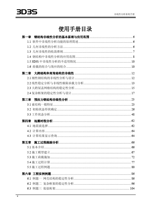
非线性分析系统手册
6.4 例题四 拉线塔..................................................................................................... 114 6.5 例题五 双层网壳施工过程分析......................................................................... 123 第七章 常见问题解答...................................................................................................... 132
第六章 工程实例例题......................................................................................................... 86 6.1 例题一 网壳结构的稳定性分析........................................................................... 86 6.2 例题二 复杂框架的稳定性分析........................................................................... 96 6.3 例题三 张弦桁架................................................................................................. 104
第四章 地震时程分析....................................................................................................... 62 4.1 地震波选择............................................................................................................. 62 4.2 计算内容................................................................................................................. 64 4.3 计算结果显示查询................................................................................................. 64