Ch02 Algorithm Analysis课件
合集下载
ch2算法分析(2)
26
【例2.3】循环次数间接依赖规模n-变量计数之二。
(1) x=1; (2) for(i=1;i<=n;i++) (3) for(j=1;j<=i;j++) (4) for(k=1;k<=j;k++) (5) x++; 该算法段中频度最大的语句是(5),从内层循环向外层分析 语句(5)的执行次数:
14
算法分类(计算时间)
多项式时间算法:可用多项式(函数)对其计 算时间限界的算法。
常见的多项式限界函数有:
Ο(1) < Ο(logn) < Ο(n) < Ο(nlogn) < Ο(n2) < Ο(n3)
指数时间算法:计算时间用指数函数限界的算 法
常见的指数时间限界函数:
Ο(2n) < Ο(n!) < Ο(nn)
30
递归方程为: T(n)=T(n-1)+O(1) 其中O(1)为一次乘法操作。 迭代求解过程如下: T(n)=T(n-2)+O(1)+O(1) =T(n-3)+O(1)+O(1)+O(1) …… =O(1)+……+O(1)+O(1)+O(1) =n*O(1) =O(n)
18
定理2 如果f(n) =am nm+.+a1n+a0 且am > 0,则 f(n)= (nm )。
该定义的优点是与O的定义对称,缺点是f(N)对 自然数的不同无穷子集有不同的表达式,且有不 同的阶时,不能很好地刻画出f(N)的下界。比如 当 100 N为正偶数 f(N)= 6N2 N为正奇数 按照定义,得到f(N)= (1),这是个平凡的下界, 对算法分析没有什么价值。
ch02

(1)流程图表示
FORTRAN语言程序设计 语言程序设计
算法- 第二章 算法-程序的关键
12
NANJING UNIVERSITY OF INFORMATION SICENCE & TECHNOLOGY
(2)N-S图表示
FORTRAN语言程序设计 语言程序设计
算法- 第二章 算法-程序的关键
13
NANJING UNIVERSITY OF INFORMATION SICENCE & TECHNOLOGY
写一个算法输入南京市2009 2009年 例 2 : 写一个算法输入南京市 2009 年5 月份每 天的平均气温, 天的平均气温,求出这个月的平均气温并 输出。 输出。
FORTRAN语言程序设计 语言程序设计
算法- 第二章 算法-程序的关键
14
NANJING UNIVERSITY OF INFORMATION SICENCE & TECHNOLOGY
(1)流程图表示
Байду номын сангаас
FORTRAN语言程序设计 语言程序设计
算法- 第二章 算法-程序的关键
15
NANJING UNIVERSITY OF INFORMATION SICENCE & TECHNOLOGY
(2)N-S图表示
FORTRAN语言程序设计 语言程序设计
算法- 第二章 算法-程序的关键
16
NANJING UNIVERSITY OF INFORMATION SICENCE & TECHNOLOGY
算法中的每一个步骤应当是确定的,无二义性; 算法中的每一个步骤应当是确定的,无二义性; 相同的输入只能得出相同的输出。 相同的输入只能得出相同的输出。
算法分析与设计PPT教学课件 Algorithms Chapter 2 算法效率分析基础

掌握算法中近似时间的表示、非递归、递归算法 的效率分析方法,了解算法的经验分析
3
分析框架——输入规模度量
输入规模度量
算法的时间效率和空间效率都用输入规模的函 数进行度量。 对于所有的算法,对于规模更大的输入都需要 运行更长的时间。 经常使用一个输入规模n为参数的函数来研究 算法的效率。 选择输入规模的合适量度,要受到所讨论算法 的操作细节影响。
12
利用极限比较增长次数
前两种情况意味着t(n) ∈ O(g(n)) 后两种情况意味着t(n) ∈ Ω(g(n)) 第二种情况意味着t(n) ∈ Θ(g(n))
P44例题
13
Graphs
f(n) is O(g(n)) cg(n) f(n)
f(n) is (g(n))
f(n) cg(n)
N
N c1g(n) f(n) c2g(n) Points to notice: What happens near the beginning (n < N) is not important cg(n) always passes through 0, but f(n) might not (why?) In the third diagram, c1g(n) and c2g(n) have the same “shape 14 ” (why?)
22
//输出:n!的值
if n=0 retuen 1 else return F(n-1)*n
举例:F(5)
分析递归算法效率的通用方案
决定用哪个参数作为输入规模的度量 找出算法的基本操作 检查对相同规模的输入,基本操作的执行 次数是否相同,如果不同,必须对最差、 平均及最优效率单独研究 建立一个递推关系式及相应的初始条件 求解这个递归关系式,或者至少确定解的 增长次数
02AlgorithmAnalysis

Map graphs in polynomial time Map graphs in polynomial time
Q. Which would you prefer 20 n100 vs. n1 + 0.02 ln n ?
Mikkel Thorup Department Mikkel Thorup of Computer Science, University of Copenhagen Universitetsparken 1, DK-2100 Copenhagen East, Denmark Department of Computer Science, University of Copenhagen mthorup@diku.dk Universitetsparken 1, DK-2100 Copenhagen East, Denmark mthorup@diku.dk Abstract AbstractChen, Grigni, and Papadimitriou (WADS’97 and STOC’98)
There exists constants c > 0 and d > 0 such that on every input of size n, its running time is bounded by c nd primitive computational steps.
choose C = 2d
how many times do you have to turn the crank?
Analytic Engine
3
Brute force
Brute force. For many nontrivial problems, there is a natural brute-force search algorithm that checks every possible solution. Typically takes 2n time or worse for inputs of size n. Unacceptable in practice.
ch02
10
Big-oh
A. Levitin “Introduction to the Design & Analysis of Algorithms,” 3rd ed., Ch. 2 © 2012 Pearson Education, Inc. Upper Saddle River, NJ. All Rights Reserved.
A. Levitin “Introduction to the Design & Analysis of Algorithms,” 3rd ed., Ch. 2 © 2012 Pearson Education, Inc. Upper Saddle River, NJ. All Rights Reserved. 5
4
Best-case, average-case, worst-case
For some algorithms efficiency depends on form of input:
Worst case: Best case:
Cworst(n) – maximum over inputs of size n Cbest(n) – minimum over inputs of size n
Example: Sequential search
Worst case
Best case
Average case
A. Levitin “Introduction to the Design & Analysis of Algorithms,” 3rd ed., Ch. 2 © 2012 Pearson Education, Inc. Upper Saddle River, NJ. All Rights Reserved. 6
CH02精品PPT课件

Y A A BC( A BC D) BC A ( A BC)(A BC D) BC ( A BC)(1 A BC D) A BC
消去法: A AB A B
L AC C D “与-或” 表达式
2、逻辑函数的化简方法
化简的主要方法: 1.公式法(代数法) 2.图解法(卡诺图法) 代数化简法: 运用逻辑代数的基本定律和恒等式进行化简的方法。
并项法: A A 1
L AB C ABC AB(C C ) AB
例: Y ABC ABC A(BC BC ) A
L (A B) (C D ) 1 ( A B)(C D )
例 Y A B (B C D)
则 Y A B (B C)D
例 Y AB C D C
则 Y (A B)C D C
注意: Δ 遵守“括号、乘、加”的运算优先次序 Δ 不属于单个变量上的反号应保留不变
3. 对偶规则:
( A C )( C D ) “或-与”表达式
“或非-或非” 表达
( A C ) ( C+D ) 式
AC CD
“与-或-非”表达式
由以上分析可知,逻辑函数有很多种表达式 形式,但形式最简洁的是与或表达式,因而也是 最常用的。
在若干个逻辑关系相同的与-或表达式中,将 其中包含的与项数最少,且每个与项中变量数最 少的表达式称为最简与-或表达式。
若 Y AB C
Y A BC
若 Y AB CD Y ( A B)(C D)
导出
必须掌握基本公式
常用公式 尽可能多掌握
常用公式
2.1.3 逻辑函数的代数化简法
从逻辑问题概括出来的逻辑函数式, 不一定是最简式。
化简电路, 就是为了降低系统的成本,提高电路的可靠性,
清华大学第二版算法分析与设计课件第一章pdf
Algorithm
An algorithm is a sequence of unambiguous instructions for solving a problem, i.e., for obtaining a required output for any legitimate input in a finite amount of time.
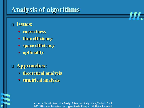
• Theoretical analysis • Empirical analysis
Optimality
Design and Analysis of Algorithms - Chapter 1 7
Algorithm design strategies
Brute force Divide and conquer Decrease and conquer Transform and conquer
Instance: The sequence <5, 3, 2, 8, 3> Algorithms:
• • • • Selection sort Insertion sort Merge sort (many others)
Design and Analysis of Algorithmsign and Analysis of Algorithms - Chapter 1
2
Notion of algorithm
problem
algorithm
input
“computer”
output
Algorithmic solution
Design and Analysis of Algorithms - Chapter 1 3
9
What is an algorithm?
An algorithm is a sequence of unambiguous instructions for solving a problem, i.e., for obtaining a required output for any legitimate input in a finite amount of time.
• Theoretical analysis • Empirical analysis
Optimality
Design and Analysis of Algorithms - Chapter 1 7
Algorithm design strategies
Brute force Divide and conquer Decrease and conquer Transform and conquer
Instance: The sequence <5, 3, 2, 8, 3> Algorithms:
• • • • Selection sort Insertion sort Merge sort (many others)
Design and Analysis of Algorithmsign and Analysis of Algorithms - Chapter 1
2
Notion of algorithm
problem
algorithm
input
“computer”
output
Algorithmic solution
Design and Analysis of Algorithms - Chapter 1 3
9
What is an algorithm?
《算法设计与分析》课件
《算法设计与分析》PPT课件
本课程将介绍算法的设计与分析,包括排序算法、查找算法和动态规划算法。 通过掌握这些算法,您将能够解决各种复杂的问题。
课程介绍
课程目标和内容概述
掌握算法设计与分析的基本概念和方法,学 习不同类型的算法及其应用。
教学方法和要求
通过理论讲解、案例分析和实际编程练习, 提高算法设计与分析的能力。
2 背包问题的动态规划解法
学习如何使用动态规划算法解决背包问题,掌握求解最优解的方法。
总结和课程评价
总结
回顾本课程涉及的算法内容,并思考所学知识 的实际应用。
课程评价
对本课程的内容、教学方法和教师的表现进行 评价和反馈。
算法基础
1 算法概述和分类
了解算法的定义、特性和常见的分类方法,为后续学习打下基础。
2 时间复杂度和空间复杂度
学习如何评估算法的时间和空间效率,并选择最合适的算法。
排序算法
1
插入排序
2
学习插排序算法的思想和实现过程,
掌握其时间复杂度和适用范围。
3
冒泡排序
掌握冒泡排序算法的原理和实现方法, 了解其时间复杂度和应用场景。
快速排序
了解快速排序算法的原理和分治思想, 学会如何选择合适的划分策略。
查找算法
顺序查找
掌握顺序查找算法的基本思想和实现过程,了 解其时间复杂度和使用场景。
二分查找
学习二分查找算法的原理和应用,了解其时间 复杂度和适用条件。
动态规划算法
1 原理和应用举例
了解动态规划算法的核心原理,并通过实例了解其在解决复杂问题时的应用。
ch 2 非对称加密算法
5
KASUMI算法 算法
RKi=KLi||KOi||KIi KLi=KLi1||KLi2 KOi=KOi1||KOi2||KOi3 KIi=KIi1||KIi2||KIi3பைடு நூலகம்KIij=KIij1(9bit)||KIij2(7bit)
6
KUSAMI-非线性盒子S7 -非线性盒子
7
KUSAMI-非线性盒子S9 -非线性盒子
16
射影平面坐标系
为了表示无穷远点,产生了射影平面坐标系, 为了表示无穷远点,产生了射影平面坐标系,它是对普通 平面直角坐标系的扩展。 平面直角坐标系的扩展。 对普通平面直角坐标系上的点A的坐标 做如下改造: 对普通平面直角坐标系上的点 的坐标(x,y)做如下改造: 的坐标 做如下改造 点可以表示为(X:Y:Z)变成 令x=X/Z ,y=Y/Z(Z≠0);则A点可以表示为 ; 点可以表示为 变成 了有三个参量的坐标点, 了有三个参量的坐标点,这就对平面上的点建立了一个新 的坐标体系。 的坐标体系。 新的直线方程: 新的直线方程:aX+bY+cZ=0,平行直线的方程是: ,平行直线的方程是: aX+bY+c1Z =0; aX+bY+c2Z =0 (c1≠c2); ; ; 有c2Z= c1Z= -(aX+bY),∵c1≠c2 ∴Z=0 ∴aX+bY=0; , ; 无穷远点就是这种形式( 无穷远点就是这种形式(X:Y:0)表示。注意,平常点 )表示。注意, Z≠0,无穷远点Z=0,因此无穷远直线对应的方程是 ,无穷远点 ,因此无穷远直线对应的方程是Z=0。 。
21
椭圆曲线中的数乘
k个相同的点 相加,记作 。如下图: 个相同的点P相加 记作kP。如下图: 个相同的点 相加, P+P+P=2P+P=3P。 。
Chapter_2_Algorithm analysis
The Maximum Subsequence Sum Problem
• 给一串整数a[1…n],求出它和最大的子序 列,即找出1<=i<=j<=n,使 a[i]+a[i+1]+…+a[j]最大 • 介绍四个算法并分析时间复杂度
0, if n=0 Fn = 1, if n=1 Fn-1 + Fn-2, if n>1
Fibonacci Numbers
• An exponential algorithm
int fib1(n) { if( n==0 ) return 0; if( n==1 ) return 1; return fib1(n-1) + fib1(n-2); }
Fibonacci Numbers
• An exponential algorithm
T(n) is exponential in n. The running time of fib1(n) is proportional to 20.694n = (1.6)n, so it takes 1.6 times to computer Fn+1 than Fn. To compute F200, the fib1 algorithm executes T(200)>=F200>=2138 elementary computer steps. For NEC Earth Simulator, which clocks 40 trillion steps per second, fastest computer in 2002, fib1(200)would take at least 292 seconds. In short, our naïve recursive algorithm is correct but hopelessly inefficient. Can we do better?
- 1、下载文档前请自行甄别文档内容的完整性,平台不提供额外的编辑、内容补充、找答案等附加服务。
- 2、"仅部分预览"的文档,不可在线预览部分如存在完整性等问题,可反馈申请退款(可完整预览的文档不适用该条件!)。
- 3、如文档侵犯您的权益,请联系客服反馈,我们会尽快为您处理(人工客服工作时间:9:00-18:30)。
instructions are executed sequentially each instruction is simple, and takes exactly one time unit integer size is fixed and we have infinite memory
• Typically the following two functions are analyzed:
பைடு நூலகம்
【Definition】 T (N) = Θ( h(N) ) if and only if T (N) = O( h(N) ) and 】 【Definition】 T (N) = o( p(N) ) if T (N) = O( p(N) ) and T (N) ≠ 】
Θ( p(N) ) .
Note:
(1) Input There are zero or more quantities that are externally supplied. (2) Output At least one quantity is produced. (3) Definiteness Each instruction is clear and unambiguous. (4) Finiteness If we trace out the instructions of an algorithm, then for all cases, the algorithm terminates after finite number of steps. (5) Effectiveness Every instruction must be basic enough to be carried out, in principle, by a person using only pencil and paper. It is not enough that each operation be definite as in(3); it also must be feasible.
/* count ++ */ return 0; /* count ++ */
}
§2 Asymptotic Notation ( Ο, Ω, Θ, o )
The point of counting the steps is to predict the growth in run time as the N change, and thereby compare the time complexities of two programs. So what we really want to know is the asymptotic behavior of Tp. Suppose Tp1 ( N ) = c1N2 + c2N and Tp2 ( N ) = c3N. Which one is faster? No matter what c1, c2, and c3 are, there will be an n0 such that Tp1 ( N ) > Tp2 ( N ) for all N > n0.
2 1 1 2 2 4 8 4 2
Input size n 4 8 16 1 1 1 2 3 4 4 8 16 8 24 64 16 64 256 64 512 4096 16 256 65536 24 40326 2092278988000
CHAPTER 2
ALGORITHM ANALYSIS 【Definition】An algorithm is a finite set of instructions 】 that, if followed, accomplishes a particular task. In addition, all algorithms must satisfy the following criteria:
/* count ++ */
Tsum ( n ) = 2n + 3
}
tempsum += list [ i ] ; /* count ++ */
/* count ++ for last execution of for */ return tempsum; /* count ++ */
〖Example〗Recursive 〗 function for summing a list of numbers Trsum ( n ) = 2n + 2
I see! So as long as I know that Tp1 is about N2 and Tp2 is about N, then for sufficiently large N, P2 will be faster!
§2 Asymptotic Notation
【Definition】 T (N) = O( f (N) ) if there are positive constants c 】
§2 Asymptotic Notation
Rules of Asymptotic Notation
If T1 (N) = O( f (N) ) and T2 (N) = O( g(N) ), then (a) T1 (N) + T2 (N) = max( O( f (N)), O( g(N)) ), (b) T1 (N) * T2 (N) = O( f (N) * g(N) ). If T (N) is a polynomial of degree k, then T (N) = Θ( N k ).
§1 What to Analyze
〖Example〗 Matrix addition 〗
void add ( int int int int { int i, j ; for ( i = 0; i < rows; i++ ) /* rows + 1 */ for ( j = 0; j < cols; j++ ) /* rows(cols+1) */ c[ i ][ j ] = a[ i ][ j ] + b[ i ][ j ]; } T(rows, cols ) = 2 rows ⋅ cols + 2rows + 1 /* rows ⋅ cols */ a[ ][ MAX_SIZE ], b[ ][ MAX_SIZE ], c[ ][ MAX_SIZE ], rows, int cols )
Sort = Find the smallest integer + Interchange it with list[i].
§1 What to Analyze
Machine & compiler-dependent run times. Time & space complexities : machine & compilerindependent. • Assumptions:
Q: What shall we do A: Exchange if rows >> cols? rows and cols.
§1 What to Analyze
〖Example〗Iterative 〗 function for summing a list of numbers
float sum ( float list[ ], int n ) { /* add a list of numbers */ float tempsum = 0; /* count = 1 */ int i ; for ( i = 0; i < n; i++ )
logk N = O(N) for any constant k. This tells us that
logarithms grow very slowly. Note: When compare the complexities of two programs asymptotically, make sure that N is sufficiently large. For example, suppose that Tp1 ( N ) = 106N and Tp2 ( N ) = N2. Although it seems that Θ( N2 ) grows faster than Θ( N ), but if N < 106, P2 is still faster than P1.
≥ 2N + 3 = O( N ) = O( Nk≥1 ) = O( 2N ) = ⋅⋅⋅ We shall always take the smallest f (N). 2N + N2 = Ω( 2N ) = Ω( N2 ) = Ω( N ) = Ω( 1 ) = ⋅⋅⋅ We shall always take the largest g(N).
Tavg(N) & Tworst(N) -- the average and worst case time complexities, respectively, as functions of input size N. If there is more than one input, these functions may have more than one argument.
§2 Asymptotic Notation
Time 1 log n n n log n n2 n3 2n n!
Name constant logarithmic linear log linear quadratic cubic exponential factorial