高宏课件Chapter1SolowGrowthModel
合集下载
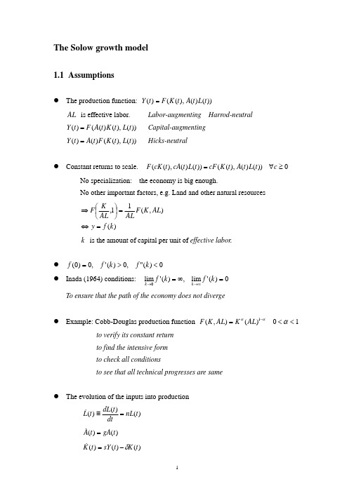
高宏课件Chapter 1 Solow Growth Model

Conditions
• These conditions imply each input is essential: F(0, L) = F(K, 0) = 0. • An example of a neoclassical production function is the Cobb-Douglas one: • Y = AKαL1-α, A > 0; 0 < α < 1. • This form implies unit elasticity of substitution between K and L. If factors paid marginal products, factor shares of income are constant at α for K and 1-α
Labor
• L = labor supply (market clears with full employment). Labor supply = population (or proportional to population). No labor leisure choice and labor-force-participation rate is constant. Can extend model to make these endogenous. • Population grows exogenously at rate n ≥ 0: (1/L)· (dL/dt) = n L(t) = L(0)· exp(nt) • Can extend model to make fertility, mortality, immigration endogenous—then n is endogenous.
高宏课件CHAPTER(1)

8.6 不确定性
8.7 金融市场的不完全性
h
11
f)
pK
(t)
其中: f为公司所得税减税比率
h
(8.5)
5
4.模型的不足之处
(1)假定资本存量调整是完全有弹性的,无成本 的,无限制的,实际上投资受限于产出规模, 因此投资和资本不可能无限连续(infinite)变 动;
(2)未考虑预期因素: 当预期需求上升或资本成 本下降时,K↑;
(3)对模型的修正: 引入资本存量的调整成本
1)内部调整成本:如安装新机器设备的成本, 训练工人操纵新机器设备的成本,利率变动 的成本等。
2)外部成本:资本h品价格的变化。
6
8.2 Q Theory Model of Investment
with Adjustment Cost
1.假定:
一产业有N个同质厂商
(1)一个典型厂商的实际利润与其资本存量(k(t))成 正比(若规模报酬不变、产品市场完全竞争、
K(t) I(t) 2. 厂商的利润函数(8.6) 即利润=收益-I-调整成本 若用离散时间,则(8.7)
h
8
预 算 约 束 : kt1 kt It
最 优 化 : (8.8) t : 资 本 的 边 际 收 益
令 q t (1 r ) t , 变 成 (8 .9 )
L : (8.10) I
为总收益, Xs:产品价格和要素成本等 假定:K 0,KK0
2.合意的资本存量的确定
K P K (K ,X 1 ,X h2 ,X 3 , ,X n ) r K 0 3
K()rK (8.1)
厂 商 合 意 的 资 本 存 量 Kf(rK,X's)
对 (8.1)式 对 rk求 导 :
高级宏观经济学索洛斯旺模型ppt课件

•.
•2
1 模型的假设
1、投入与产出:①生产函数的形式为Y(t)=F[K(t), A(t)L(t)]。资本K、劳动L、知识A(或称“劳动有效性”) 为投入,将各种投入结合在一起,即可以生产出产品Y。
②时间不直接进入生产函数,仅当投入随时间发生变化 时,产量才随时间发生变化。
③AL可称为有效劳动,以此种形式引入的技术称为 “哈罗德中性”技术。本模型采用“哈罗德中性”技术。
中的规模报酬不变假设.将生产函数改写为密集形式.
FcK,cAL cK cAL1 cc1K AL 1 cFK, AL
f
k
f
AKL,1
K AL
k.
容易验证: f 'k0, f ''k0
•.
•5
1 模型的假设
3、三种投入品变动的假设: ①劳动和知识以不变速度增长,L(t)= L(0)ent或
dL(t)/dt= nL(t), A(t)= A(0)ent或dA(t)/dt= gA(t) 。 ②储蓄率s是外生的,现存资本的折旧率为б ,于
•.
•8
2 k的动态方程
将有效劳均总投资与持平投次 表示为k的函数。可得右上图。
右上图中,由于f(0)=0,因此, 当k=0时,实际投资与持平投 资相等。
稻田条件意味着当k=0时, f‘(k)很大,因而,实际投资曲 线陡于持平投资曲线。
稻田条件也意味着k很大时, k
f‘(k)趋近于0。 随着实际投资曲线变得平坦,
•.
•12
4 储蓄率变化的影响
如果f 'k * n g ,那么0
4 储蓄率变化的影响
1、对产量的影响:储蓄率s的增加会使实际投资 曲线向上移动,因此k*上升,但到达新的k*值后, 它又将保持不变。
高级宏观经济学索洛斯旺模型ppt课件

高级宏观经济学索洛斯旺模型ppt 课件
contents
目录
• 索洛-斯旺模型概述 • 索洛-斯旺模型中的经济增长 • 储蓄、投资与资本积累 • 劳动生产率、技术进步与经济增长 • 政策因素对索洛-斯旺模型的影响 • 索洛-斯旺模型在现实世界的应用 • 总结与展望
01 索洛-斯旺模型概述
模型背景与意义
03 储蓄、投资与资本积累
储蓄函数及影响因素
01
储蓄函数的定义与性质
02
储蓄是可支配收入减去消费的部分
储蓄函数描述了储蓄与可支配收入之间的关系
03
储蓄函数及影响因素
收入越高,储蓄倾向越大
收入水平
影响因素
01
03 02
储蓄函数及影响因素
利率水平 利率上升,储蓄增加;利率下降,储蓄减少
储蓄函数及影响因素
经济增长路径的特点
经济增长路径具有收敛性、稳定性和 动态性等特点。其中收敛性是指不同 经济体在长期中趋向于相同的稳态均 衡状态;稳定性是指经济增长路径在 受到外部冲击时能够保持相对稳定; 动态性是指经济增长路径随着技术进 步和制度变迁等因素的变化而不断调 整。
经济增长路径的政策 含义
经济增长路径的政策含义在于,政府 可以通过调整经济政策来影响经济增 长的路径和速度。例如,通过提高投 资率、促进技术进步、优化产业结构 等措施来加快经济增长;同时,也需 要关注经济增长带来的资源环境压力 和社会公平问题,实现可持续发展。
03
加强教育和科技创新投入,提高人力资本 积累水平。
04
推进产业结构调整和升级,优化资源配置 效率。
04 劳动生产率、技术进步与 经济增长
劳动生产率提升途径
教育和培训
通过提高劳动者的知识和技能水平,提升劳动 生产率。
L3_Solow_augmenting_technology

Consumption per unit of effective labor: c (t ) = (1 − s )y (t ) Investment per unit of effective labor: i (t ) = sy (t ) Output per unit of effective labor: y (t ) = f [k (t )] The fundamental law of motion of the Solow model: ˙ (t ) = sf [k (t )] − (n + g + δ )k (t ) k
A Permanent Increase in the Saving Rate
∗ ] − (n + g + δ ) ≤ 0 Case 1: snew f [kold
0.16 0.14 0.12
Small Increase in the Saving Rate
ሶ
0.1 0.08 0.06 0.04 0.02 0
Essentiality: f (0) = 0
f (0) = F [0, 1] = 0
Unboundedness: lim f [k ] = ∞
k →∞
K →∞ K lim F [K , AL] = AL lim F [ AL , 1] = AL lim f [k ]
K AL →∞
k →∞
Equilibrium
+δ − n+g =0 s
(k ∗ )2
Using Implicit Function Theorem, we can obtain
Q /∂ s n+g +δ = − ∂∂Q /∂ k ∗ = − s 2
高级宏观经济学 02 The Solow growth model
( ) ( ) ⇒ sf ' k∗ ∂k∗ + f k∗ = (n + g + δ ) ∂k∗
∂s
∂s
⇒
∂k ∗ ∂s
=
(n +
g
f (k∗ )
+ δ )− sf
'(k∗ )
⇒
∂y∗ ∂s
=
f '(k∗ )f (k∗ ) (n + g + δ )− sf '(k∗ )
( ) k∗ f ' k∗
( )( ( ) ) ( ( ) ) ⇒
z f (0) = 0, f '(k) > 0, f "(k) < 0
z Inada (1964) conditions: lim f '(k) = ∞, lim f '(k) = 0
k →0
k →∞
To ensure that the path of the economy does not diverge
z The saving rate is exogenous in the Solow model z The impact on output:
z The long-run effect
k The effect of an increase in the saving rate on
investment
∂y∗ ∂s
s y∗
= 1−k∗ f '
f k∗
k∗ f k∗
=
1
αK −α
k
K
∗
k
∗
4
( ) z
Empirical evidence shows: αK k∗
高宏课件Chapter 1 Solow Growth Model

高宏课件Chapter 1 Solow Growth Model
# 高宏课件Chapteห้องสมุดไป่ตู้ 1 Solow Growth Model
简介
描述S olow增长模型的意义和应用,解释其重要组成部分。 Introduce the significance and applications of the Solow Growth Model and explain its important components.
总结
S olow模型的优缺点,S olow模型在经济增长研究中的价值,S olow模型的未来应用和发展趋势。 Summary: strengths and weaknesses of the Solow Model, its value in economic growth research, and future applications and development trends.
Solow模型概述
S olow模型的基本假设,生产函数和边际产出,稳态状态和收敛性。 Overview of the Solow Model: assumptions, production function and marginal output, steady state and convergence.
模型应用
S olow模型在各种经济系统中的应用,特定假设下的计算,政策建议的制定。 Applications of the Solow Model: its use in various economic systems, calculations under specific assumptions, formulation of policy recommendations.
最新高宏课件Chapter 1 Solow Growth Model精品资料

• Y = F(K, L, t). • Common assumption to get nice steady-state
results, when n = (1/L)·(dL/dt) is constant, is that technical progress takes labor augmenting, Kaldor form. Y depends on K and effective labor, • Lˆ = L·φ(t) Y = F(K, Lˆ ).
• An example of a neoclassical production function is the Cobb-Douglas one:
• Y = AKαL1-α, A > 0; 0 < α < 1. • This form implies unit elasticity ond Model Structure
• Production:Neoclassical production function: Y = F(K, L, A).
• A: non-rival, non-excludible technology. • One-sector technology: Y goes for C or ΔK (gross investment). • K, capital, is cumulated net investment. Can interpret K to include human capital. K depreciates at rate δ > 0 (exogenous).
extend model to make these endogenous.
• Population grows exogenously at rate n ≥ 0:
- 1、下载文档前请自行甄别文档内容的完整性,平台不提供额外的编辑、内容补充、找答案等附加服务。
- 2、"仅部分预览"的文档,不可在线预览部分如存在完整性等问题,可反馈申请退款(可完整预览的文档不适用该条件!)。
- 3、如文档侵犯您的权益,请联系客服反馈,我们会尽快为您处理(人工客服工作时间:9:00-18:30)。
• An example of a neoclassical production function is the Cobb-Douglas one:
• Y = AKαL1-α, A > 0; 0 < α < 1. • This form implies unit elasticity of substitution
between K and L. If factors paid marginal products, factor shares of income are constant at α for K and 1-α
Technological progress
• Basic model assumes exogenous technological progress—A depends only on time, t:
• Y = F(K, L, t). • Common assumption to get nice steady-state
results, when n = (1/L)·(dL/dt) is constant, is that technical progress takes labor augmenting, Kaldor form. Y depends on K and effective labor, • Lˆ = L·φ(t) Y = F(K, Lˆ ).
Chapter1SolowGrowthModel
Factsabouteconomicgrowth; Assumptionandmodelstructure; Dynamics;Comparativestatic;Conver gence;Dataandgrowthaccounting;Ho
meworkandpaper
About A
• If technical change takes place at constant rate
• x ≥ 0, Lˆ= L exp(xt), • Lˆ grows at rate n + x. • Technology might instead augment K
(Solow) or F(K, L) overall (Hicks). If production function is Cobb-Douglas, the three forms are indistinguishable.
Properties of neoclassical
production function
• Constant returns to scale (CRS) in K, L: F(λK, λL, A) =λ·F(K, L, A) for allλ >0
• Positive and diminishing marginal products: FK , FL > 0; FKK, FLL < 0.
• L = labor supply (market clears with full employment). Labor supply = population (or proportional to population). No labor leisure choice and labor-force-participation rate is constant. Can extend model to make these endogenous.
• Limiting (Inada) conditions:
• Lim (FK) = ∞, Lim (FFK) = 0, Lim (FL) = 0;
• K→∞
L→∞
Conditions
• These conditions imply each input is essential: F(0, L) = F(K, 0) = 0.
1 Facts and key questions
• Growth rates differ: as China,US, Africa; • Productivity growth slowdown; • See Pictures • Key question: what drives economic growth • Key question 2:why it differ so much? • Now we start with Solow model • Question:Why starts with Solow?
• Population grows exogenously at rate n ≥ 0:
• (1/L)·(dL/dt) = n
L(t) = L(0)·exp(nt)
• Can extend model to make fertility, mortality, immigration endogenous—then n is endogenous.
Model Structure
• Standard model has labor-augmenting technical change at constant rate, x.
2Assumptions and Model Structure
• Production:Neoclassical production function:
•
Y = F(K, L, A).
• A: non-rival, non-excludible technology.
• One-sector technology: Y goes for C or ΔK
• (gross investment).
• K, capital, is cumulated net investment. Can
• interpret K to include human capital. K
• depreciates at rate δ > 0 (exogenous).
Labor