曼昆经济学原理Chapter13企业行为与产业组织 中英文笔记
《经济学原理·曼昆·第三版》第13章
30*5%=1.5
10*5%=0.5 20*5%=1
--20*5%=1
13.1.4 经济利润与会计利润 Economic Profit versus Accounting Profit
economic profit —— the firm’s total revenue minus all the opportunity costs (explicit and implicit) of producing the goods and services sold. 经济利润——企业的总收益减生产所销售物品与劳务的所 有机会成本
greater quantity of a good when the price of the good is higher, and this response leads to a supply curve that slopes upward. For analyzing many questions, the law of supply is all you need to know about firm behavior. In this chapter and the ones that follow, we examine firm behavior in more detail. This topic will give you a better understanding of what decisions lie behind the supply curve in a market. In addition, it will introduce you to a part of economics
How an Economist Views a Firm
曼昆-十大经济学原理,中英文对照
曼昆-十大经济学原理,中英文对照第一篇:曼昆-十大经济学原理,中英文对照十大经济学原理。
曼昆在《经济学原理》一书中提出了十大经济学原理,他们分别是:十大经济学原理一:人们面临权衡取舍。
人们为了获得一件东西,必须放弃另一件东西。
决策需要对目标进行比较。
People Face Trade offs.To get one thing, you have to give up something else.Making decisions requires trading off one goal against another.例子:这样的例子很多,典型的是在“大炮与黄油”之间的选择,军事上所占的资源越多,可供民用消费和投资的资源就会越少。
同样,政府用于生产公共品的资源越多,剩下的用于生产私人品的资源就越少;我们用来消费的食品越多,则用来消费的衣服就越少;学生用于学习的时间越多,那么用于休息的时间就越少。
十大经济学原理二:某种东西的成本是为了得到它所放弃的东西。
决策者必须要考虑其行为的显性成本和隐性成本。
The Cost of Something is what You Give Up to Get It.Decision-makers have to consider both the obvious and implicit costs of their actions.例子:某公司决定在一个公园附近开采金矿的成本。
开采者称由于公园的门票收入几乎不受影响,因此金矿开采的成本很低。
但可以发现伴随着金矿开采带来的噪声、水和空气的污染、环境的恶化等,是否真的不会影响公园的风景价值?尽管货币价值成本可能会很小,但是考虑到环境和自然生态价值会丧失,因此机会成本事实上可能很大。
十大经济学原理三:理性人考虑边际量。
理性的决策者当且仅当行动的边际收益超过边际成本时才采取行动。
Rational People Think at Margin.A rational decision-makertakes action if and only if the marginal benefit of the action exceeds the marginal cost.例子:“边际量”是指某个经济变量在一定的影响因素下发生的变动量。
竞争市场中的企业(经济学原理-曼昆-中英文双语)
P = MR1 = MR2
MC
ATC
P = AR = MR
AVC
MC1
0
Q1
QMAX
Q2
Quantity
Copyright © 2004 South-Western
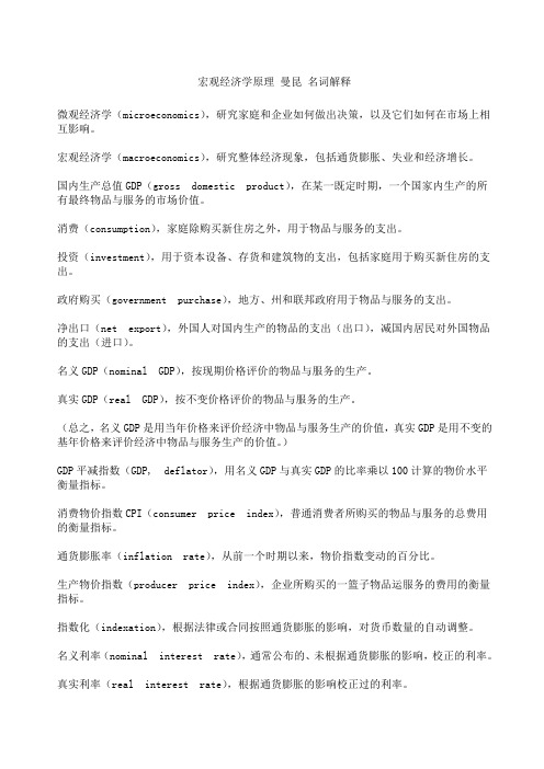
图1. 竞争企业的利润最大化
成本 和
收益
MC2
通过生产边际成本等于 边际收益的产量,企业 使利润最大化
P=MR1
MC1
MC
ATC P = AR = MR AVC
0
Q1
QMAX Q2
产量
Profit Maximization for the Competitive Firm 竞争企业的利润最大化
Profit maximization occurs at the quantity where marginal revenue equals marginal cost. 当边际收益等于边际成本时,企业实 现利润最大化。
Harcourt, Inc. items and derived items copyright © 2001 by Harcourt, Inc.
什么是竞争市场?
完全竞争市场有以下特点 :
市场中有许多买者和许多卖者。 各个卖者所提供的物品大体上是相同的。 企业可以自由地进入或退出市场。
Harcourt, Inc. items and derived items copyright © 2001 by Harcourt, Inc.
总成本 (TC) $3.00 $5.00 $8.00 $12.00 $17.00 $23.00 $30.00 $38.00 $47.00
利润 (TR-TC) -$3.00 $1.00 $4.00 $6.00 $7.00 $7.00 $6.00 $4.00 $1.00
宏观经济学原理第七版曼昆名词解释带英文
宏观经济学原理曼昆名词解释微观经济学(microeconomics),研究家庭和企业如何做出决策,以及它们如何在市场上相互影响。
宏观经济学(macroeconomics),研究整体经济现象,包括通货膨胀、失业和经济增长。
国内生产总值GDP(gross domestic product),在某一既定时期,一个国家内生产的所有最终物品与服务的市场价值。
消费(consumption),家庭除购买新住房之外,用于物品与服务的支出。
投资(investment),用于资本设备、存货和建筑物的支出,包括家庭用于购买新住房的支出。
政府购买(government purchase),地方、州和联邦政府用于物品与服务的支出。
净出口(net export),外国人对国内生产的物品的支出(出口),减国内居民对外国物品的支出(进口)。
名义GDP(nominal GDP),按现期价格评价的物品与服务的生产。
真实GDP(real GDP),按不变价格评价的物品与服务的生产。
(总之,名义GDP是用当年价格来评价经济中物品与服务生产的价值,真实GDP是用不变的基年价格来评价经济中物品与服务生产的价值。
)GDP平减指数(GDP, deflator),用名义GDP与真实GDP的比率乘以100计算的物价水平衡量指标。
消费物价指数CPI(consumer price index),普通消费者所购买的物品与服务的总费用的衡量指标。
通货膨胀率(inflation rate),从前一个时期以来,物价指数变动的百分比。
生产物价指数(producer price index),企业所购买的一篮子物品运服务的费用的衡量指标。
指数化(indexation),根据法律或合同按照通货膨胀的影响,对货币数量的自动调整。
名义利率(nominal interest rate),通常公布的、未根据通货膨胀的影响,校正的利率。
真实利率(real interest rate),根据通货膨胀的影响校正过的利率。
曼昆经济学原理chapt1-chapt15笔记整理
Chapter 1: Introduction前言1. Society allocates people to various jobs and the output of goods and services.2. Scarcity means that resources are limited so cannot produce all the goods and services people want.3. Economics is the study of how society manages its scare resources.4. Economists study 3 things:·How people make decisions·How people interact with one another·Analyze forces and trends that affect the economy as a wholeHow people make decisions (10 principles)1. People face trade-off1) Making decisions requires trading off one goal against another.2) Trade-off society faces:·Guns and butter; a clean environment and a high level of income·Efficiency and equityàmaximum benefits and fair2. The cost of sth is what you give up to get it1) Opportunity cost: what you give up to get that item3. Rational people think at the margin1) They systematically and purposefully do the best to achieve their objectives2) Marginal changes are adjustments around the edges of what you are doing3) Rational people make decisions by comparing marginal benefits and costs4) People’s willingness to pay for any good is the marginal benefit of an extra unit of the good wouldbring4. People respond to incentives1) Public policymakersàincentivesàpolicies change people’s behavior. E.g. taxHow people interact5. Trade can make everyone better off1) Allow countries to specialize in what they do best and to enjoy more goods6. Markets are usually a good way to organize economic activity1) Market economy is more successful2) The invisible hand is price which adjust to maximize the welfare of society7. Governments can sometimes improve market outcomes1) Reasons why we need G·Invisible hand works only if property rights are enforced·Invisible hand is powerful but not omnipotent全能的; policies aim to promote both efficiency and equityàMarket failureàa situation in which the market on its own fails to produce an efficient allocation of resources. Causes: externality and market power·Invisible hand fail to ensure that economic prosperity is distributed equitablyHow the economy as a whole works8. A country’s standard of living depends on its ability to produce goods and services1) Productivityàthe quantity of goods and services produced from each hour of a worker’stimeàproductivity high, living standard high2) Far-reaching and public policy will implicate the relationship between productivity and livingsrandard9. Prices rise when the G prints too many money1) Keep inflation at a low level2) Growth in the amount of money causes inflation10. Society faces a short-run trade-off between inflation and unemployment1) Business cycleàfluctuations in economic activity, such as employment and productionChapter 2: Thinking like an economist1. The scientific method: observationàtheoryàmore observationàadvanced theory2. Economists make assumptions because they can simplify the complex world and make it easier tounderstand3. Economists use diff. assumptions to answer diff. Qs4. Economists use models, which are built with assumptions and composed of diagrams and equations,to learn about the worldModel 1: the circular-flow diagramàonly two types of decision makersàfirms and householdsModel 2: the production possibilities frontier1) The shape of PPF is bowed outward2) On PPFàefficiency level of production; In or out off PPTàinefficiency3) PPF shows the opportunity cost of one good as measured in terms of the other good4) The opportunity cost of products’ quantity is reflected in the shape of the PPF5. Positive VS normative analysisPS: descriptive; claims about how the world isàscientistsNS: prescriptive; claims about how the world ought to beàpolicy advisers6. The field of economics is divided into microeconomics and macroeconomics7. Differences in scientific judgments or values cause the conflictions between economists who advisepolicymakerChapter 4: The market forces of supply and demandMarket and competition1. Market1) Buyers and sellersàdemand and supply2) Highly organized and less organized marketàagricultural commodities and ice cream market2. Perfectly competition market1) Goods are exactly the same2) So numerous buyers and sellersàno single one will influence the market price3) Buyers and sellers are price takers, and can buy or sell all they want4) e.g. wheat market, ice cream market5) Economists use the model of supply and demand to analyze this marketDemand1. Quantity demanded: the amount of good that buyers are willing and able to buy1) The quantity demanded is negatively related to the priceàprice rises, quantity demandedfallsàprice affect a movement along the demand curve2) Market demand is the sum of all the individuals demands for a good2. Demand curve: what happens to the quantity demanded of a good when the price varies3. Curve shifts when there is a change in a relevant variable that is not measured on either axis4. Shifts in demand curve (right, increase in demand; left, decrease)1) Income·Normal good (include necessity and luxury): income fallsàdemand falls (positive correlation); e.g.ice cream·Inferior good: income fallsàdemand rises (negative correlation); e.g. to ride a bus2) Prices of related goods·Substitutes: price of one good falls, demand of another good reduceàpairs of goods in place of each other; e.g. hot dogs and hamburgers·Complements: price of one good falls, demand of another good raisesàpairs of goods used together; e.g. computer and software3) Tastes: the most obvious determinant of the demand; likeàbuy more4) Expectations·Expect higher incomeàsave lessàbuy more today·Expect higher priceàbuy more today5) Numbers of buyers: more members, shift to rightSupply1. Quantity supplied is the amount that sellers are willing and able to sellàpositive related to the good’spriceàchange of price lead to supply’s change2. Market supply is the sum of the supplies of all sellersàadd all of the suppliers3. Shifts in the supply curve1) Input pricesàinput’s price rises substantially, shift to left2) Technologyàadvance in technology, raise the supply3) Expectationsàfirm, price rise in the future, supply less4) Number of sellersàmore members, higher supplyEquilibrium1. Equilibrium: market piece has reached the level at which quantity supplied=quantity demandedàthequantity of goods buyers are willing and able to buy=sellers are willing and able to sell2. Equilibrium price=market-clearing priceàeveryone in the market has been satisfiedàdetermines howmuch of the good buyers choose to purchase and how much sellers choose to produce3. Actual price>E priceàsurplus=excess supplyàquantity supplied>quantity demandedàsellers cut thepriceàincrease quantity demanded and decrease quantity supplied4. Market price<E priceàshortage=excess demandàquantity supplied<quantity demandedàsellers raisethe priceàquantity demanded falls and quantity supplied rises5. Law of supply and demand: the price of any good adjusts to bring the quantity supplied and quantitydemanded for that good into balance6. How quickly prices adjust determine how quickly equilibrium is reached; vary from market to market7. Surpluses and shortages in free market are temporaryThree steps to analyzing changes in E1. Decide whether the events shifts the supply or demand curve (or perhaps both)2. Decide in which direction the curve shifts3. Use the supply-and-demand diagram to see how the shift changes the equilibrium price and quantity(compare new E with the initial E)4. A shift in the supply/demand curve=change in supply/demand; a movement along a fixedsupply/demand curve=change in the quantity supplied/demandedConclusion1. Supply and demand together determine the prices of goods, price in turn guide the allocation ofresources2. Prices determine who buys each good and how much is producedChapter 5: Elasticity and its applicationThe price elasticity of demand3. A larger price elasticityàa greater responsiveness of quantity demanded to price4. Midpoint method: a better wayPrice elasticity of demand=[(Q2-Q1)/(Q2+Q1)]/[(P2-P1)/(P2+P1)]5. The variety of demand curves: the flatter the demand curve that passes through a given point, thegreater the price elasticity of demand1) Perfectly inelastic: elasticity=0, demand curve is vertical2) Inelastic: elasticity<1, demand curve seems steepPrice and total revenue move in the same direction3) Unit elasticity: elasticity=1Total revenue remains constant when the price change4) Elastic: elasticity>1, demand curve seems flatPrice and total revenue move in opposite directions5) Perfectly elastic: elasticity=infinity, demand curve is horizontal6. The slope of a linear demand curve=1 while the elasticity is not the same along the entire curve.7. Other demand elasticity1) The income elasticity of demand=% change in quantity demand/% change in income·Normal goodsàpositive income elasticityàquantity demanded and income move in the same direction·Necessities: small elasticity(无论income如何变化,需求可理解成基本不变)·Luxuries: large elasticity·Inferior goodsànegative income elasticityàin opposite directions2) The cross-price elasticity of demand=% change in quantity demanded of good1/% change in theprice of good2·Substitutesàthe cross-price elasticity is positive·ComplementsànegativeThe price elasticity of supply1. Determinant of the price elasticity of supply: time periodàmore elastic in the long time2. Price elasticity of supply=% change in quantity supplied/% change in price (midpoint method or not…)3. The variety of supply curves1) Perfectly inelastic: elasticity=0, supply curve is vertical2) Inelastic: elasticity<1, supply curve seems steep3) Unit elasticity: elasticity=14) Elastic: elasticity>1, supply curve seems flat5) Perfectly elastic: elasticity=infinity, supply curve is horizontal4. Max capacity for productionàthe elasticity of supply may be high at low levels of quantity supplied andlow at high levels of quantity suppliedChapter 6: Supply, demand and G policiesControls on price1. Price ceiling: a legal max. on the price at which a good can be sold1) E price<ceilingàprice ceiling is not bindingàprice ceiling has no effect on the price or the quantitysold2) E price>ceilingàceiling is a binding constraintàshortage (or larger shortage)àsellers ration the scaregoodsàinefficiency (wasting time and discrimination)3) E.g. gas pump, rent control etc.2. Price floor: a legal min. on the price at which a good can be sold1) E price>flooràprice floor is not bindingàprice floor has no effect2) E price<flooràbinding constraintàsurplus3) E.g. min. wageàunemploymentTax1. Tax levied on buyers1) Supply curve is not affected2) Shift the demand curve downward (not to left)3) Implications·Taxes discourage market activityàquantity sold is smaller·Buyers and sellers share the burden of taxes (see P125, figure 6)àbuyers pay more and sellers receive less2. Tax levied on sellers1) Demand curve does not change2) Shift the supply curve upward3) Implications are identical with the implications in “Tax levied on buyers”3. Elasticity and tax incidence1) Supply is more elastic than demandàthe incidence of the tax falls more heavily on consumers thanon producers2) 反之亦然Chapter 7: Consumers, producers and the efficiency of markets前言1. Welfare economics is the study of how the allocation of resources affects economic well-being2. The basic tools of welfare economics are consumer and producer surplus3. The equilibrium of supply and demand in a market max. the total benefits received by buyers andsellersConsumer surplus1. Consumer surplus=the amount a buyer is willing to pay for a good – the amount the buyer actually payfor itàthe area below the demand curve/above the price2. Consumer surplus measures the benefit that buyers receive from a good as the buyers themselvesperceive it3. Lower priceàadditional initial and new consumer surplusàhigher consumer surplus4. In most markets, consumer surplus reflect economic well-being (assume buyers are rational);exception: in drug marketProducer surplus1. Producer surplus=the amount a seller is paid – the cost of productionàthe area below the price andabove the supply curve2. Producer surplus measures the benefit to sellers of participating in a market (sellers’ well-being)3. Higher priceàadditional producer surplus to initial and new producersàhigher producer surplus Market efficiency1. One way to measure the economic well-being of a society:Total surplus=consumer surplus + producer surplus=value to buyers – amount paid by buyers + amount received by sellers – cost to sellers (amount paid by buyers=amount received by sellers)=values to buyers – cost to sellers2. Efficiency: an allocation of resources maximizes total surplusàwhether the pie is as big as possible3. Equity: the fairness of the distribution of well-being among the members of societyàwhether the pie isdivided fairly4. 3 insights about market outcomes1) Free market allocate the supply of goods to the buyers who value them most highly, as measuredby their willingness to pay2) Free markets allocate the demand for goods to the sellers who can produce them at least cost3) Free markets produce the quantity if goods that max. the sum of consumer and producer surplus Conclusion1. All buyers and sellers are together led by an invisible hand to an equilibrium that max. the totalbenefits to buyers and sellers2. All the analyses and the conclusion above are based on two assumptions·Markets are perfectly competitive·The outcome in a market matters only to the buyers and sellers in that market3. The presence of market failure, such as market power and externalities, leads to the inability of someunregulated markets to allocate resources efficiency4. If markets fail, public policy can remedy (cope with) the problem and increase economic efficiency Chapter 10: Externalities前言1. Externality: the uncompensated无补偿的impact of one person’s actions on the well-being of abystander (the effect of when a transaction between a buyer and a seller directly affects a third party) ·Adverse impactànegative externalityàe.g. pollution·Beneficial impactàpositive externalityàe.g. education2. Externalitiesàmarket equilibrium is not efficientàequilibrium fails to max. the total benefit to society asa whole3. Policyàdeal with the market failureExternalities and market inefficiency1. Negative externalities1) Social cost=private cost + external costàupward of supply curveàoptional quantity<market quantity2) To achieve the optional outcomeàtax for productsàupward the supply curveàtax accuratelyreflected the social costànew supply curve=social-cost curve2. Internalizing the externality: altering incentives so that people take account of the external effects oftheir actions (e.g. tax)3. Positive externalities1) Positive externalities of education·More informed votersàbetter G·Lower crime rates·Encourage the development and dissemination of tech.àhigher productivity and wages2) Social value=private value + external benefitàupward of demand curveàoptional quantity>marketquantity3) Subsideàmove the market equilibrium closer to the social optimumPrivate solutions to externalities1. Typesàto internalize externalities1) Moral codes and social sanctions2) Charities3) Rely on the self-interest of the relevant parties4) Enter into a contract for the interested parties2. The coase theorem: if private parties can bargain without cost over the allocation of resources, theycan solve the problem of externalities on their own3. Drawback of private solutions1) The coase theorem applies only when the interested parties have no trouble reaching andenforcing an agreement2) Transaction cost is the costs that parties incur in the process if agreeing to and following throughon a bargain (e.g. language difference)Public policies toward externalities1. When people cannot solve the problem, the G steps in2. Command-and-control policiesàregulation3. Market-based policy1) Corrective taxes and subsidiesàincentive to develop tech.·Corrective taxes=Pigovian taxes: a tax designed to induce private decision makers to take account of the social costs that arise from a negative externality2) Tradable pollution permitsChapter 13: The costs of production前言1. Industrial organization: the study of how firms’ decisions about prices and quantity depend on themarket condition they face2. The costs of the firm are a key determinant of its production and pricing decision3. Firms’ goal: max. profitCosts1. Total revenue=quantity X priceàthe amount that the firm receives for the sale of its output2. Economic Profit=total revenue – all the opportunity cost=total revenue – (explicit cost + implicit cost)3. Accounting profit=total revenue - explicit cost4. Explicit/implicit cost: input costs that require/do not require an outlay of money by the firmProduction and costsàthe link between a firm’s production process and its total cost in short run1. A firm’s cost reflect its production process2. Production function: the relationship between quantity of input and the quantity of output of thegoodàflatter as the increase of the input3. Marginal product (the production function’s slope): the increase in output that arises from anaddition al unit of inputàdiminishing MP: the input’s MP declines as the increase input4. Total-cost curve: the relationship between total cost and quantity of outputàopposite sides comparedwith production functionàsteeper as the increase of outputMeasures of cost1. Total cost=fixed costs + variable costs·Fixed/Variable costs: costs that do not/do vary with the quantity of output produced2. ATC=TC/Qàthe cost of a typical unit of output if total cost is divided evenly over all the units produced3. MC=∆TC/∆Qàthe increase in TC that arises from producing an additional unit of output4. Shapes of cost curves(characteristics)1) MCàrisingàreflect the property of diminishing marginal product2) ATCàU-shapedàreflect both fixed and variable costs’ shapes·The bottom of ATC=min. TCàthis quantity=efficient scale3) MC and ATC cross at the bottom of ATC·MC<ATC, ATC is falling·MC>ATC, ATC is risingCost in the short run and long run1. Costs are fixed or variable costs now will change depending on the time horizon2. Long-run ATC and short-run ATC·Long-run curve is a much flatter U-shape than the short-run curve·All short-run curves lie on or above the long-run curveàfirms’ greater flexibility in long-run3. How long it takes for a firm to get to the long run depends on the firm4. Scaleàshape of the long-run curve1) Economies of scaleàoutput increase, ATC declines2) Constant returns to scaleàATC does not vary with the level of output3) Diseconomies of scaleàoutput increase, ATC rises5. Causes of economies or dis-e of scale·Specializationàhigher production levelàrise economies of scale·Coordination problems in large org.àmore stretchedàrise dis-e of scale6. When the firm changes its level of production, ATC rises more in the short run than in the long run7. A firm’s cost curve do not tell what decisions the firm will make while is important component of thedecisionsChapter 14: Firms in competitive marketsWhat is a competitive market1. Competitive market=perfectly competitive market, characteristics:·Many buyers and sellers·Goods sold are largely the same·Firms can freely enter or exit the market2. Total revenue=P X Q; Average revenue=TR/QàAR=P3. MR=∆TR/∆QàMC=P4. AR=MR=PProfit max. and firms’ supply curve1. Firm is a price takeràprice line is horizontalàMR line is horizontal2. At the profit-maximizing level of output, MR=MC·Why not MC=ATC?àlowest total cost≠max. profit, do not forget revenue3. MC curve determines the quantity of the good the firm is willing to supply at any price, the MC curve=firm’s supply curve, while is t he different portion1) Short-run decisionàif the value get from the producing<VCàshut down·If TR<VCàTR/Q<VC/QàP/AVC·The firm’s short-run supply curve is the portion of its MC curve lies above AVC2) Sunk cost: a cost that has already been committed and cannot be recoveredàthe opposite ofopportunity cost·Ignore the sunk cost when deciding how to produce or whether to shut down in short run3) Long-run decisionà if the value get from the producing<ATCàexit·If TR<TCàTR/Q<TC/QàP<ATCàexit (if P>ATC, new firms enter)·The firm’s long-run supply curve is the portion of its MC curve lies above ARC4. Long run: Profit=(P – ATC)XQ; Loss=(ATC-P)XQThe supply curve in a competitive market1. Short runàdifficult to enter or exitàfixed number of firms·Every firm’s MC curve is its supply curve·Firms are identicalàsum of quantity in MC curve=market quantity2. Long run àthe process of entry and exit ends only when price=ATCàfirms remain in the market mustbe making zero economic profit1) P=MC=min. ATCàthe long-run equilibrium of a competitive market with free entry and exit musthave firms operating at their efficient scale2) Firms adjust to ensure that all demand is satisfied at the price (min.ATC)àlong-run market supplycurve is horizontal at this price3. Economic profit is zero ≠ accounting profit is zeroàfirms stay in firms if they make zero profit4. A shift in demand1) Start: long-run equilibrium2) Short run: demand increaseàP rises, Q rises (compared with start)àprofit3) Long run: more firmsàsupply increaseàP unchanged, Q rises (compared with start)àzero-profitequilibrium5. Reasons why long-run curve may slope upward1) Some resources used in production may be available only in limited quantities (e.g. land)2) Firms may have different cost (e.g. some people work faster)6. Firms can enter or exit more easily in the long run than short runàlong-run supply curve is moreelasticChapter 15: MonopolyWhy monopoly (barriers to entry)1. Monopoly resourcesàa key resources or there are no close substitutes, e.g. diamond2. Govt-created monopoliesàG has given one person or firm the exclusive right to sell some good orservice3. Natural monopoliesàa single firm can supply a good to an smaller cost than could two or more firms·May be determined by the market sizeHow monopoly makes production and pricing decisions1. A monopolyàsole produceràit can alter the price of its good by adjusting the quantity it supplied tothe market2. A competitive firm can sell all it wantsàdemand curve is horizontalA monopolist’s demand curve is its market demand curveàdownward3. Monopoly: downward-sloping demand curveàMR<P (reduce revenue on the units it was alreadyselling)·当垄断者增加一单位生产时,它就必须降低对所销售的每一单位产品收取的价格,而且,这种价格下降减少了它已经迈出的个单位的收益·The MC=P at start4. When MC=MR, the quantity is the profit-maximizing quantityàprice at this quantity is the monopolypriceàP>MR=MC5. A monopoly’s profit=TR-TC=(TR/Q-TC/Q)Q=(P-ATC)QThe welfare cost of monopoly1. Monopoly price>marginal costànot all consumers who value the good at more than its cost buyitàmonopoly quantity<efficient quantityàdeadweight loss2. Welfare=consumers welfare + producers welfare1) In monopoly market, money transfers from consumers to producersàthe sum of total surplus is notaffected2) The market is efficient but not equity3) The firm produces smaller quantityàdeadweight loss=how much the economic pieshrinksàinefficientPublic policies toward monopolies1. Increasing competition with antitrust lawsàpromote competition and the problem of synergies(merger)2. Regulationànatural monopolies are not allowed to charge any price they wantThe problems1) Natural monopolies’ ATC curve is declining and marginal cost is less than ATCàloss·Subsidizes the monopolist·Allows the monopolist to charge a P>MC2) It gives the monopolist no incentive to reduce costs3. Public ownershipàthe G can run the monopoly itselfe.g. some Gs own and operate utilities such as telephone, water, electric companies4. Doing nothingPrice discrimination: the business practice of selling the same good at different prices to different consumers (can either raise or lower welfare)1. Three lessonsàhigher producer surplus rather than higher consumers surplus1) The price discrimination is a rational strategy for a profit-maximizing monopolistàmonopolist canincrease its profit2) Price discrimination requires the ability to separate customers according to their willingness topayàmay have the problem of arbitrage3) Price discrimination can raise economic welfare2. Perfect price discrimination: a situation in which the monopolist knows exactly the willingness to payof each customer and can charge each customer a different priceàno deadweight lossàmonopoly producer gains all the wntire surplus in the form of profit3. The price discrimination raises the monopoly’s profit to some extent4. Examples of price discrimination·Movie tickets·Airline prices·Discount coupons·Financial aid·Quantity discountConclusion1. Monopolies are common2. Firms with substantial monopoly power are rareàfew goods are truly unique3. Monopoly power is a matter of degreeàmonopoly power sometimes is limited。
曼昆的《微观经济学基础》课业笔记 英文版
曼昆的《微观经济学基础》课业笔记英文版IntroductionThis document presents my notes on "Microeconomics: Principles and Applications" by N. Gregory Mankiw. These notes summarize key concepts and ideas covered in the book, aiming to provide a helpful overview of microeconomics.Chapter 1: Ten Principles of Economics- People face trade-offs: individuals and societies must make choices due to scarcity.- The cost of something is what you give up to get it: when making decisions, considering both the direct and opportunity costs is crucial.- Rational people think at the margin: making decisions by evaluating incremental benefits and costs.- People respond to incentives: incentives can influence individuals' behavior and decision-making.- Trade can make everyone better off: voluntary exchange benefits all parties involved.- Markets are usually a good way to organize economic activity: markets coordinate exchanges efficiently.- A country's standard of living depends on its ability to produce goods and services: productivity is key.- Prices rise when the government prints too much money: inflation can be caused by excessive money supply growth.- Society faces a short-run trade-off between inflation and unemployment: the Phillips curve illustrates this trade-off.Chapter 2: Thinking Like an Economist- Economists use models to simplify reality and understand economic behavior.- Assumptions in economic models help focus on essential elements.- Opportunity cost is the true cost of something and is measured by what we give up to obtain it.Chapter 3: Interdependence and the Gains from Trade- Specialization and international trade result in greater production efficiency and consumption possibilities.- Both parties benefit from trade even if one has an absolute advantage in both goods.- Prices reflect the opportunity cost and guide resources to their most valued uses.Chapter 4: The Market Forces of Supply and Demand- Markets consist of buyers and sellers, and their interactions determine prices and quantities.- Demand curve shows the relationship between price and quantity demanded, while supply curve reflects the relationship between price and quantity supplied.- Market equilibrium occurs when quantity demanded equals quantity supplied.- Changes in demand or supply shift their respective curves, leading to changes in equilibrium price and quantity.ConclusionThese notes provide a brief summary of the key concepts covered in "Microeconomics: Principles and Applications." Studying this bookallows for a deeper understanding of microeconomic principles and their applications in the real world.。
曼昆经济学原理英文版文案加习题答案13章

221WHAT’S NEW IN THE S EVENTH EDITION:There are no major changes to this chapter.LEARNING OBJECTIVES:By the end of this chapter, students should understand:➢ what items are included in a firm’s costs of production.➢ the link between a f irm’s production process and its total costs.➢ the meaning of average total cost and marginal cost and how they are related.➢ the shape of a typical firm’s cost curves.➢ the relationship between short-run and long-run costs.CONTEXT AND PURPOSE:Chapter 13 is the first chapter in a five-chapter sequence dealing with firm behavior and the organization of industry. It is important that students become comfortable with the material in Chapter 13 because Chapters 14 through 17 are based on the concepts developed in Chapter 13. To be more specific, Chapter 13 develops the cost curves on which firm behavior is based. The remaining chapters in thissection (Chapters 14-17) utilize these cost curves to develop the behavior of firms in a variety of different market structures —competitive, monopolistic, monopolistically competitive, and oligopolistic.The purpose of Chapter 13 is to address the costs of production and develop the firm’s cost curves. These cost curves underlie the firm’s supply curve. In previous chapters, we summarized the firm’s production decisions by starting with the supply curve. While this is suitable for answering manyquestions, it is now necessary to address the costs that underlie the supply curve in order to address the part of economics known as industrial organization —the study of how firms’ decisions about prices and quantities depend on the market conditions they face.KEY POINTS:•The goal of firms is to maximize profit, which equals total revenue minus total cost.THE COSTS OF PRODUCTION13222 ❖Chapter 13/The Costs of Production• When analyzing a firm’s behavior, it is important to include all the opportunity costs of production.Some of the opportunity costs, such as the wages a firm pays its workers, are explicit. Otheropportunity costs, such as the wages the firm owner gives up by working at the firm rather than taking another job, are implicit. Economic profit takes both explicit and implicit costs into account, whereas accounting profits consider only explicit costs.• A firm’s costs reflect its production process. A typical firm’s production function gets flatter as the quantity of an input increases, displaying the property of diminishing marginal product. As a result, a firm’s total-cost curve gets steeper as the quantity produced rises.• A firm’s total costs can be divided between fixed costs and variable costs. Fixed costs are costs that do not change when the firm alters the quantity of output produced. Variable costs are costs that change when the firm alters the quantity of output produced.• From a firm’s total cost, two related measures of cost are derived. Average total cost is total cost divided by the quantity of output. Marginal cost is the amount by which total cost rises if output increases by one unit.• When analyzing firm behavior, it is often useful to graph average total cost and marginal cost. For a typical firm, marginal cost rises with the quantity of output. Average total cost first falls as output increases and then rises as output increases further. The marginal-cost curve always crosses the average-total-cost curve at the minimum of average total cost.• A firm’s costs often depend on the time horizon considered. In particular, many costs are fixed in the short run but variable in the long run. As a result, when the firm changes its level of production, average total cost may rise more in the short run than in the long run.CHAPTER OUTLINE:I. What Are Costs?A. Total Revenue, Total Cost, and Profit1. The goal of a firm is to maximize profit.Chapter 13/The Costs of Production ❖ 2232. Definition of total revenue: the amount a firm receives for the sale of its output.3. Definition of total cost: the market value of the inputs a firm uses in production.4. Definition of profit: total revenue minus total cost.B. Costs as Opportunity Costs1. Principle #2: The cost of something is what you give up to get it.2. The costs of producing an item must include all of the opportunity costs of inputs used inproduction. 3. Total opportunity costs include both implicit and explicit costs.a. Definition of explicit costs: input costs that require an outlay of money by thefirm .b. Definition of implicit costs: input costs that do not require an outlay of moneyby the firm .c. The total cost of a business is the sum of explicit costs and implicit costs.d. This is the major way in which accountants and economists differ in analyzing theperformance of a business. e. Accountants focus on explicit costs, while economists examine both explicit and implicitcosts.C. The Cost of Capital as an Opportunity Cost 1. The opportunity cost of financial capital is an important cost to include in any analysis of firmperformance. 2. Example: Caroline uses $300,000 of her savings to start her firm. It was in a savings accountpaying 5% interest.3. Because Caroline could have earned $15,000 per year on this savings, we must include thisopportunity cost. (Note that an accountant would not count this $15,000 as part of the firm's costs.)224 ❖ Chapter 13/The Costs of Production4. If Caroline had instead borrowed $200,000 from a bank and used $100,000 from her savings,the opportunity cost would not change if the interest rate stayed the same (according to the economist). But the accountant would now count the $10,000 in interest paid for the bank loan.D. Economic Profit versus Accounting Profit1. Figure 1 highlights the differences in the ways in which economists and accountants calculateprofit. 2. Definition of economic profit: total revenue minus total cost, including both explicitand implicit costs .a. Economic profit is what motivates firms to supply goods and services.b. To understand how industries evolve, we need to examine economic profit. 3. Definition of accounting profit: total revenue minus total explicit cost .4. If implicit costs are greater than zero, accounting profit will always exceed economic profit.II. Production and CostsA. The Production Function1. Definition of production function: the relationship between quantity of inputs usedto make a good and the quantity of output of that good.2. Example: Caroline's cookie factory. The size of the factory is assumed to be fixed; Carolinecan vary her output (cookies) only by varying the labor used.Chapter 13/The Costs of Production ❖ 2253. Definition of marginal product: the increase in output that arises from an additionalunit of input.a. As the amount of labor used increases, the marginal product of labor falls.b. Definition of diminishing marginal product: the property whereby the marginalproduct of an input declines as the quantity of the input increases.4. We can draw a graph of the firm's production function by plotting the level of labor (x -axis)against the level of output (y -axis).226 ❖Chapter 13/The Costs of ProductionFigure 2a. The slope of the production function measures marginal product.b. Diminishing marginal product can be seen from the fact that the slope falls as theamount of labor used increases.B. From the Production Function to the Total-Cost Curve1. We can draw a graph of the firm's total cost curve by plotting the level of output (x-axis)against the total cost of producing that output (y-axis).a. The total cost curve gets steeper and steeper as output rises.b. This increase in the slope of the total cost curve is also due to diminishing marginalproduct: As Caroline increases the production of cookies, her kitchen becomesovercrowded, and she needs a lot more labor.Chapter 13/The Costs of Production ❖227III. The Various Measures of CostA. Example: Conrad’s Coffee Shop228 ❖Chapter 13/The Costs of ProductionB. Fixed and Variable Costs1. Definition of fixed costs: costs that do not vary with the quantity of outputproduced.2. Definition of variable costs: costs that do vary with the quantity of output produced.3. Total cost is equal to fixed cost plus variable cost.C. Average and Marginal Cost1. Definition of average total cost: total cost divided by the quantity of output.2. Definition of average fixed cost: fixed costs divided by the quantity of output.3. Definition of average variable cost: variable costs divided by the quantity of output.4. Definition of marginal cost: the increase in total cost that arises from an extra unitof production.Chapter 13/The Costs of Production ❖ 2295. Average total cost tells us the cost of a typical unit of output and marginal cost tells us thecost of an additional unit of output.D. Cost Curves and Their Shapes1. Rising Marginal Costa. This occurs because of diminishing marginal product.b. At a low level of output, there are few workers and a lot of idle equipment. But as outputincreases, the coffee shop gets crowded and the cost of producing another unit of output becomes high.2. U-Shaped Average Total Costa. Average total cost is the sum of average fixed cost and average variable cost.b. AFC declines as output expands and AVC typically increases as output expands. AFC ishigh when output levels are low. As output expands, AFC declines pulling ATC down. As fixed costs get spread over a large number of units, the effect of AFC on ATC falls and ATC begins to rise because of diminishing marginal product. c. Definition of efficient scale: the quantity of output that minimizes average totalcost. 3. The Relationship between Marginal Cost and Average Total Costa. Whenever marginal cost is less than average total cost, average total cost is falling.Whenever marginal cost is greater than average total cost, average total cost is rising.b. The marginal-cost curve crosses the average-total-cost curve at minimum average totalcost (the efficient scale).230 ❖ Chapter 13/The Costs of Production4. Typical Cost Curvesa. Marginal cost eventually rises with output.b. The average-total-cost curve is U-shaped.c. Marginal cost crosses average total cost at the minimum of average total cost.Activity 2—Average and Marginal GradesType: In-class demonstration Topics: Relationship between marginal and average cost Materials needed: None Time: 5 minutes Class limitations: Works in any size classPurposeThis quick exercise uses an analogy to illustrate to students that they already know the relation between marginal values and averages.InstructionsTell the class that two twins (Miley and Hannah) are enrolled in Principles of Economics. They each had a “B” average (GPA = 3.0) before taking the class.Miley gets a “C” in the course. What happens to her GPA?Hannah gets an “A” in the class. What happens to her GPA?Common Answers and Points for DiscussionStudents will likely know that Miley will have a lower GPA and Hannah a higher GPA. A “marginal” grade lower than the average will pull down the average. A “marginal” grade higher than the average will increase the average.The same is true of marginal cost and average costs. If marginal cost is less than average cost, average cost will fall. If marginal cost is higher than average cost, average cost will rise. Figure 5IV. Costs in the Short Run and in the Long RunA. The division of total costs into fixed and variable costs will vary from firm to firm.B. Some costs are fixed in the short run, but all are variable in the long run.1. For example, in the long run a firm could choose the size of its factory.2. Once a factory is chosen, the firm must deal with the short-run costs associated with thatplant size.C. The long-run average-total-cost curve lies along the lowest points of the short-run average-total-cost curves because the firm has more flexibility in the long run to deal with changes in production.D. The long-run average-total-cost curve is typically U-shaped, but is much flatter than a typicalshort-run average-total-cost curve.E. The length of time for a firm to get to the long run will depend on the firm involved.F. Economies and Diseconomies of Scale1. Definition of economies of scale: the property whereby long-run average total costfalls as the quantity of output increases.2. Definition of diseconomies of scale: the property whereby long-run average totalcost rises as the quantity of output increases.3. Definition of constant returns to scale: the property whereby long-run average totalcost stays the same as the quantity of output changes.Figure 6 Emphasize that these cost curves include ALL costs for the resources needed toproduce the good. Thus, both explicit costs and implicit costs are included.4. FYI: Lessons from a Pin Factorya. In The Wealth of Nations, Adam Smith described how specialization in a pin factoryallowed output to be greater than it would have been if each worker attempted toperform many different tasks.b. The use of specialization allows firms to achieve economies of scale.V. Table 3 provides a summary of all of the various cost definitions used throughout this chapter.Table 3SOLUTIONS TO TEXT PROBLEMS:Quick Quizzes1. Farmer McDonald’s opportunity c ost is $300, consisting of 10 hours of lessons at $20 an hourthat he could have been earning plus $100 in seeds. His accountant would only count theexplicit cost of the seeds ($100). If McDonald earns $200 from selling the crops, thenMcDonald earns a $100 accounting profit ($200 sales minus $100 cost of seeds) but incursan economic loss of $100 ($200 sales minus $300 opportunity cost).2. Farmer Jones’s production function is shown in Figure 1 and his total-cost curve is shown inFigure 2. The production function becomes flatter as the number of bags of seeds increasesbecause of the diminishing marginal product of seeds. The total-cost curve gets steeper asthe amount of production increases. This feature is also due to the diminishing marginalproduct of seeds, since each additional bag of seeds generates a lower marginal product, andthus, the cost of producing additional bushels of wheat rises.Figure 1 Figure 23. The average total cost of producing 5 cars is $250,000/5 = $50,000. Since total cost rosefrom $225,000 to $250,000 when output increased from 4 to 5, the marginal cost of the fifthcar is $25,000.The marginal-cost curve and the average-total-cost curve for a typical firm are shown inFigure 3. They cross at the efficient scale because at low levels of output, marginal cost isbelow average total cost, so average total cost is falling. But after the two curves cross,marginal cost rises above average total cost, and average total cost starts to rise. So thepoint of intersection must be the minimum of average total cost.Figure 34. The long-run average total cost of producing 9 planes is $9 million/9 = $1 million. The long-run average total cost of producing 10 planes is $9.5 million/10 = $0.95 million. Since thelong-run average total cost declines as the number of planes increases, Boeing exhibitseconomies of scale.Questions for Review1. The relationship between a firm's total revenue, profit, and total cost is profit equals totalrevenue minus total costs.2. An accountant would not count the owner’s opportunity cost of alternative employment as anaccounting cost. An example is given in the text in which Caroline runs a cookie business, butshe could instead work as a computer programmer. Because she's working in her cookiefactory, she gives up the opportunity to earn $100 per hour as a computer programmer. Theaccountant ignores this opportunity cost because money does not flow into or out of the firm.But the cost is relevant to Caroline’s decision to run the cookie factory.3. Marginal product is the increase in output that arises from an additional unit of input.Diminishing marginal product means that the marginal product of an input declines as thequantity of the input increases.4. Figure 4 shows a production function that exhibits diminishing marginal product of labor.Figure 5 shows the associated total-cost curve. The production function is concave becauseof diminishing marginal product, while the total-cost curve is convex for the same reason.Figure 4 Figure 55. Total cost consists of the costs of all inputs needed to produce a given quantity of output. Itincludes fixed costs and variable costs. Average total cost is the cost of a typical unit ofoutput and is equal to total cost divided by the quantity produced. Marginal cost is the cost of producing an additional unit of output and is equal to the change in total cost divided by the change in quantity. An additional relation between average total cost and marginal cost is that whenever marginal cost is less than average total cost, average total cost is declining;whenever marginal cost is greater than average total cost, average total cost is rising.Figure 66. Figure 6 shows the marginal-cost curve and the average-total-cost curve for a typical firm.There are three main features of these curves: (1) marginal cost is U-shaped but risessharply as output increases; (2) average total cost is U-shaped; and (3) whenever marginal cost is less than average total cost, average total cost is declining; whenever marginal cost is greater than average total cost, average total cost is rising. Marginal cost is increasing for output greater than a certain quantity because of diminishing returns. The average-total-cost curve is downward-sloping initially because the firm is able to spread out fixed costs over additional units. The average-total-cost curve is increasing beyond some output levelbecause as quantity increases, the demand for important variable inputs increases; therefore, the cost of these inputs increases. The marginal-cost and average-total-cost curves intersect at the minimum of average total cost; that quantity is the efficient scale.7. In the long run, a firm can adjust the factors of production that are fixed in the short run; forexample, it can increase the size of its factory. As a result, the long-run average-total-costcurve has a much flatter U-shape than the short-run average-total-cost curve. In addition,the long-run curve lies along the lower envelope of the short-run curves.8. Economies of scale exist when long-run average total cost decreases as the quantity ofoutput increases, which occurs because of specialization among workers. Diseconomies ofscale exist when long-run average total cost rises as the quantity of output increases, whichoccurs because of the coordination problems inherent in a large organization.Quick Check Multiple Choice1. a2. d3. d4. c5. b6. aProblems and Applications1. a. opportunity cost; b. average total cost; c. fixed cost; d. variable cost; e. total cost; f.marginal cost.2. a. The opportunity cost of something is what must be given up to acquire it.b. The opportunity cost of running the hardware store is $550,000, consisting of $500,000to rent the store and buy the stock and a $50,000 implicit cost, because your aunt wouldquit her job as an accountant to run the store. Because the total opportunity cost of$550,000 exceeds the projected revenue of $510,000, your aunt should not open thestore, as her economic profit would be negative.3. a. The following table shows the marginal product of each hour spent fishing:b. Figure 7 graphs the fisherman's production function. The production function becomesflatter as the number of hours spent fishing increases, illustrating diminishing marginalproduct.Figure 7c. The table shows the fixed cost, variable cost, and total cost of fishing. Figure 8 showsthe fisherman's total-cost curve. It has an upward slope because catching additional fish takes additional time. The curve is convex because there are diminishing returns tofishing time because each additional hour spent fishing yields fewer additional fish.Figure 84. Here is the completed table:Workers Output MarginalProduct TotalCostAverageTotal CostMarginalCost0 0 --- $200 --- ---1 20 20 300 $15.00 $5.002 50 30 400 8.00 3.333 90 40 500 5.56 2.504 120 30 600 5.00 3.335 140 20 700 5.00 5.006 150 10 800 5.33 10.007 155 5 900 5.81 20.00a. See the table for marginal product. Marginal product rises at first, then declines becauseof diminishing marginal product.b. See the table for total cost.c. See the table for average total cost. Average total cost is U-shaped. When quantity is low,average total cost declines as quantity rises; when quantity is high, average total costrises as quantity rises.d. See the table for marginal cost. Marginal cost is also U-shaped, but rises steeply asoutput increases. This is due to diminishing marginal product.e. When marginal product is rising, marginal cost is falling, and vice versa.f. When marginal cost is less than average total cost, average total cost is falling; the costof the last unit produced pulls the average down. When marginal cost is greater thanaverage total cost, average total cost is rising; the cost of the last unit produced pushesthe average up.5. At an output level of 600 players, total cost is $180,000 (600 × $300). The total cost ofproducing 601 players is $180,901. Therefore, you should not accept the offer of $550,because the marginal cost of the 601st player is $901.6. a. The fixed cost is $300, because fixed cost equals total cost minus variable cost. At anoutput of zero, the only costs are fixed cost.Marginal cost equals the change in total cost for each additional unit of output. It is also equal to the change in variable cost for each additional unit of output. This relationshipoccurs because total cost equals the sum of variable cost and fixed cost and fixed costdoes not change as the quantity changes. Thus, as quantity increases, the increase intotal cost equals the increase in variable cost.7. The following table illustrates average fixed cost (AFC), average variable cost (AVC), andaverage total cost (ATC) for each quantity. The efficient scale is 4 houses per month,because that minimizes average total cost.Quantity VariableCost FixedCostTotalCostAverageFixed CostAverageVariable CostAverageTotal Cost0 $0.00 $200.00 $200.00 --- --- ---1 10.00 200.00 210.00 $200.00 $10.00 $210.002 20.00 200.00 220.00 100.00 10.00 110.003 40.00 200.00 240.00 66.67 13.33 80.004 80.00 200.00 280.00 50.00 20.00 70.005 160.00 200.00 360.00 40.00 32.00 72.006 320.00 200.00 520.00 33.33 53.33 86.677 640.00 200.00 840.00 28.57 91.43 120.008. a. The lump-sum tax causes an increase in fixed cost. Therefore, as Figure 10 shows, onlyaverage fixed cost and average total cost will be affected.Figure 10b. Refer to Figure 11. Average variable cost, average total cost, and marginal cost will all begreater. Average fixed cost will be unaffected.Figure 119. a. The following table shows average variable cost (AVC), average total cost (ATC), andmarginal cost (MC) for each quantity.Quantity VariableCost TotalCostAverageVariable CostAverageTotal CostMarginalCost0 $0.00 $30.00 --- --- ---1 10.00 40.00 $10.00 $40.00 $10.002 25.00 55.00 12.50 27.50 15.003 45.00 75.00 15.00 25.00 20.004 70.00 100.00 17.50 25.00 25.005 100.00 130.00 20.00 26.00 30.006 135.00 165.00 22.50 27.50 35.00b. Figure 12 shows the three curves. The marginal-cost curve is below the average-total-cost curve when output is less than four and average total cost is declining. Themarginal-cost curve is above the average-total-cost curve when output is above four and average total cost is rising. The marginal-cost curve lies above the average-variable-cost curve.Figure 1210. The following table shows quantity (Q), total cost (TC), and average total cost (ATC) for thethree firms:Firm A Firm B Firm CQuantity TC ATC TC ATC TC ATC1 $60.00 $60.00 $11.00 $11.00 $21.00 $21.002 70.00 35.00 24.00 12.00 34.00 17.003 80.00 26.67 39.00 13.00 49.00 16.334 90.00 22.50 56.00 14.00 66.00 16.505 100.00 20.00 75.00 15.00 85.00 17.006 110.00 18.33 96.00 16.00 106.00 17.677 120.00 17.14 119.00 17.00 129.00 18.43Firm A has economies of scale because average total cost declines as output increases. Firm B has diseconomies of scale because average total cost rises as output rises. Firm C has economies of scale from one to three units of output and diseconomies of scale for levels of output beyond three units.。
曼昆经济学原理读书笔记
曼昆《经济学原理》读书笔记(8)应用原理6买者对一种物品的支付意愿与需求曲线之间的联系如何定义并衡量消费者剩余卖者生产一种物品的成本与供给曲线之间的联系如何定义并衡量生产者剩余供给与需求均衡可以使市场总剩余最大关键概念(Key Concepts):1.福利经济学welfare economicsthe study of how the allocation of resources affects economic well-being.2.支付意愿willingness to paythe maximum amount that a buyer will pay for a good.3.消费者剩余consumer surplusa buyer’s willingness to pay minus the amount the buyer actually pays.4.生产者剩余producer surplusthe amount a seller is paid for a good minus the seller’s cost.5.成本costthe value of everything a seller must give up to produce a good.6.效率efficiencythe property of a resource allocation of maximizing the total surplus received by all members of society.7.平等equitythe fairness of the distribution of well-being among the members of society.第七章消费者、生产者与市场效率CONSUMERS, PRODUCERS,AND THE EFFICIENCY OF MARKETS一、消费者剩余1、福利经济学研究资源配置如何影响经济福利。
- 1、下载文档前请自行甄别文档内容的完整性,平台不提供额外的编辑、内容补充、找答案等附加服务。
- 2、"仅部分预览"的文档,不可在线预览部分如存在完整性等问题,可反馈申请退款(可完整预览的文档不适用该条件!)。
- 3、如文档侵犯您的权益,请联系客服反馈,我们会尽快为您处理(人工客服工作时间:9:00-18:30)。
Chapter 13 The Costs of Production 生产成本§1. 什么是成本What are costs?一.Total revenue, Total cost & Profit 总收入、总成本和利润1.企业的目标是利润最大化The economic goal of the firm is to maximize profits.2.总收入Total revenue:企业出售产品所得到的货币量the amount that the firm receives for the sale of its output3.总成本Total cost:企业用于生产的投入品的市场价值the market value of the inputs a firm uses in production4.利润Profit:总收入-总成本Total revenue - Total cost二.作为机会成本的成本Costs as Opportunity Costs1.一个企业的生产成本包括生产物品与劳务量的所有机会成本A firm’s cost of production includes all the opportunity costs of making its output of goods and services.2.显性成本Explicit costs:要求企业直接支付货币的投入要素成本input costs that require a direct outlay of money by the firm3.隐性成本Implicit costs:不要求企业支付货币的投入要素成本input costs that do not require an outlay of money by the firm4.结论:经济学家既考虑显性成本又考虑隐形成本,会计师负责记录流入企业和流出企业的货币,因此他们衡量显性成本忽略隐形成本三.作为一种机会成本的资本成本The Cost of Capital as An Opportunity Costs 已经投资于企业的金融资本的机会成本是一项重要的隐形成本四.经济利润与会计利润Economic Profit versus Accounting Profit1.经济利润Economic Profit:经济学家衡量,即企业总收益减去生产所销售物品与服务的总机会成本(显性的+隐性的)Economists measure a firm’s economic profit as total revenue minus all the opportunity costs (explicit and implicit).2.会计利润:会计师衡量,即企业的总收益减去企业的显性成本Accountants measure the accounting profit as the firm’s total revenue minus only the firm’s explicit costs. In other words, they ignore the implicit costs.3.由于会计师忽略了隐形成本,所以经济利润小于会计利润Economic profit is smaller than accounting profit.4.当总收益大于显性成本和隐性成本时,企业赚取经济利润When total revenue exceeds both explicit and implicit costs, the firm earns economic profit.5.经济利润是企业供给物品与服务的动机所在,获得正经济利润的企业将继续经营§2. 生产与成本Production And Costs一.生产函数The Production Function1.生产函数Production Function:用于生产一种物品的投入量与该物品的产量之间的关系the relationship between quantity of inputs used to make a good and the quantity of output of that good2.边际产量Marginal Product:增加一单位投入所引起的产量增加the increase in the quantity of output obtained from an additional unit of that input ·计算公式:Marginal Product = Additional output ÷Additional input即:边际产量= 产出增加量÷投入增加量3.边际产量递减Diminishing Marginal Product:一种投入要素的边际产量随着投入量增加而减少的特征the property whereby the marginal product of an input declines as the quantity of the input increases例:由于雇佣的工人越来越多,每个新雇佣的工人对产量的贡献越来越小,这是因为有限的设备数量不能将他的潜能发挥出来。
结论:1.生产函数的斜率衡量了一种投入要素(比如一个工人)的边际产量。
2.随着工人数量增加,边际产量减少,生产函数越来越平坦。
二.从生产函数到总成本曲线From the Production Function to the Total-Cost Curve1.总成本曲线total-cost curve:用来说明生产产量和生产总成本之间关系的图shows the relationship between the quantity a firm can produce and its costs graphically2.结论:随着产量增加,总成本曲线越来越陡峭△对比:随着产量的增加,生产函数却越来越平坦§3. 成本的各种衡量指标The Various Measures of Cost一.固定成本与可变成本Fixed Costs and Variable Costs1.固定成本Fixed Costs:不随产量变动而变动的成本costs that do not vary with the quantity of output produced2.可变成本Variable Costs:随着产量变动而变动的成本costs that do change as the firm alters the quantity of output produced二.总成本Total Costs1.总固定成本Total Fixed Costs (TFC)2.总可变成本Total Variable Costs (TVC)3.总成本Total Costs (TC)4.关系:总成本= 总固定成本+总可变成本TC = TFC + TVC三.平均成本Average Costs:总成本除以产量(是生产一个普通单位的成本)determined by dividing the firm’s costs by the quantity of output produced1.平均固定成本Average Fixed Costs (AFC) =固定成本除以产量2.平均可变成本Average Variable Costs (AVC) =可变成本除以产量3.平均总成本Average Total Costs (ATC) =总成本除以产量4.关系:平均总成本= 平均固定成本+平均可变成本ATC = AFC + AVC四.边际成本Marginal Cost(MC):额外一单位所引起的总成本增加measures the amount total cost rises when the firm increases production by one unit ·计算:边际成本=总成本变化/产量变化=ΔTC /ΔQ结论:1.边际成本随着产量增加而上升2.边际成本递增反映了边际产量递减的性质reflects the property of diminishing marginal product五.成本曲线及其形状Cost Curves and Their Shapes·四条曲线:ATC平均总成本、AFC平均固定成本、AVC平均可变成本、MC边际成本1.U形平均总成本曲线:因为平均总成本是平均固定成本与平均可变成本之和。
在产量水平极低时,平均总成本高,这是因为固定成本只分摊在少数几个单位产品上。
平均总成本随着产量增加而降低。
当平均可变成本大幅度上升时,平均总成本开始增加。
在使平均总成本最小的产量时,U型曲线的底部就出现了。
这种产量被称为有效规模△有效规模efficient scale:使平均总成本最小的产量2.边际成本(MC)与平均总成本(ATC)之间的关系:只要边际成本小于平均总成本,平均总成本就下降。
只要边际成本大于平均总成本,平均总成本就上升。
边际成本曲线与平均总成本曲线在平均总成本曲线的最低点(有限规模)处相交。
The marginal-cost curve crosses the average-total-cost curve at the efficient scale.六.典型的成本曲线Typical Cost Curves·成本曲线的三个重要特征:1.随着产量增加,边际成本最终要上升2.平均总成本曲线是U型的3.边际成本曲线与平均总成本曲线在平均总成本最低点相交§4. 短期成本与长期成本COSTS IN THE SHORT RUN AND IN THE LONG RUN一.定义:总成本在固定成本和可变成本之间的划分取决于时间范围the division of total costs between fixed and variable costs depends on the time horizon 在短期中一些成本是固定的In the short run, some costs are fixed.在长期中成本都是可变的In the long run, fixed costs become variable costs二.规模经济与规模不经济Economies and Diseconomies of Scale1.定义:当长期平均总成本随着产量增加而减少时,存在规模经济Economies of scale当长期平均总成本随着产量增加而增加时,存在规模不经济Diseconomies of scale 当长期平均总成本不随着产量变动而变动时,存在规模收益不变Constant returns to scale2.结论:长期平均总成本曲线的形状反映了成本如何随着一个企业的经营规模变动。