ABAQUS实体单元内力输出
abaqus中实体单元的内力提取方法汇总
实体单元建的模型,要提取截面的内力有什么好方法呢?我看过别人的一个帖:对于一般的实体单元结构可以定义surface 然后用section file 输出其中,这个surface可以在cae中定义,也可以在inp中定义,但是由于涉及到边的编号问题,所以在inp中容易出错。
section file 的结果直接在dat中可见。
需要编制小程序将其数据提取。
一定要编个程序才可以提取吗在dat文件里没有找到什么section file是输出在*.fil文件中。
要直接得到截面的total force,moment,heat flux可以在inp中添加:*SECTION PRINT,name=*,surface=**SOF,SOM在dat文件中可以找到总内力和弯矩我做钢筋混凝土的问题,模型分为两个part,分别是钢筋和混凝土,然后Assembe在一起,将钢筋embeded到混凝土内。
我在keywords编辑器End assemble前定义*surface, type=cutting surface,name=surface_1-21.5,0,0,1,0,0怎么也不成,总说定义的截面没有相交(坐标计算没有错误)。
第三行空着(帮助文档说表示截断整个模型)也不行,写上钢筋或混凝土的单元组名(没有另建组,直接用的keywords编辑器中钢筋或混凝土生成单元的组名)也不行。
请问是怎么回事?哪位有相关的例子给我一个,我的QQ:40735053。
还望不吝赐教,谢谢。
Displaying a free body cutYou can define a free body cut to view the resultant forces and moments transmitted across a selected surface of a model. Force vectors are displayed with a single arrowhead and moment vectors with a double arrowhead.To create a free body cut:1. To display the entire model in the viewport, select Tools Display Group Plot All fromthe main menu bar.2. From the main menu bar, select Tools Free Body Cut Manager.3. Click Create in the Free Body Cut Manager.4. From the dialog box that appears, select 3D element faces as the Selection method andclick Continue.5. In the Free Body Cross-Section dialog box, select Surfaces as the Item and Pick fromviewport as the Method.6. In the prompt area, set the selection method to by angle and accept the default angle.7. Select the surface, highlighted in Figure 4–33, to define the free body cut cross-section.a. From the Selection toolbar, toggle off the Select the Entity Closest to theScreen tool and ensure that the Select From All Entities tool is selected.b. As you move the cursor in the viewport, Abaqus/CAE highlights all of the potentialselections and adds ellipsis marks (...) next to the cursor arrow to indicate an ambiguousselection. Position the cursor so that one of the faces of the desired surface ishighlighted, and click to display the first surface selection.Figure 4–33 Selected faces for the free body cross-section.c. Use the Next and Previous buttons to cycle through the possible selections until theappropriate vertical surface is highlighted, and click OK.8. Click Done in the prompt area to indicate your selection is complete. Click OK in the FreeBody Cross-Section dialog box.9. In the Edit Free Body Cut dialog box, accept the default settings for the SummationPoint and the Component Resolution. Click OK to close the dialog box.10. Click Options in the Free Body Cut Manager.11. From the Free Body Plot Options dialog box, select the Force tab in the Color &Style tabbed page. Click the resultant color sample to change the color of the resultant force arrow.12. Once you have selected a new color for the resultant force arrow, click OK in the Free BodyPlot Options dialog box and click Dismiss in the Free Body Cut Manager.The free body cut is displayed in the viewport, as shown in Figure 4–34.Figure 4–34 Free body cut displayed on the connecting lug.Generating tabular data reports for subsets of the modelTabular output data were generated earlier for this model using printed output requests. However, for complicated models it is convenient to write these data for selected regions of the model using Abaqus/Viewer. This is achieved using display groups in conjunction with the report generation feature. For the connecting lug problem we will generate the following tabular data reports: •Stresses in the elements at the built-in end of the lug (to determine the maximum stress in the lug)•Reaction forces at the built-in end of the lug (to check that the reaction forces at the constraints balance the applied loads)•Vertical displacements at the bottom of the hole (to determine the deflection of the lug when the load is applied)Each of these reports will be generated using display groups whose contents are selected in the viewport. Thus, begin by creating and saving display groups for each region of interest.To create and save a display group containing the elements at the built-in end:1. In the Results Tree, double-click Display Groups.2. Choose Elements from the Item list and Pick from viewport as the selection method.3. Restore the option to select entities closest to the screen.4. In the prompt area, set the selection method to by angle; and click the built-in face of the lug.Click Done when all the elements at the built-in face of the lug are highlighted in the viewport.In the Create Display Group dialog box, click Replace followed by Save As. Save thedisplay group as built-in elements.To create and save a display group containing the nodes at the built-in end:1. In the Create Display Group dialog box, choose Nodes from the Item list and Pick fromviewport as the selection method.2. In the prompt area, set the selection method to by angle; and click the built-in face of the lug.Click Done when all the nodes on the built-in face of the lug are highlighted in the viewport. In the Create Display Group dialog box, click Replace followed by Save As. Save thedisplay group as built-in nodes.To create and save a display group containing the nodes at the bottom of the hole:1. In the Create Display Group dialog box, select All from the item list, and click Replace toreset the active display group to include the entire model.2. In the Create Display Group dialog box, choose Nodes from the Item list and Pick fromviewport as the selection method.3. In the prompt area, set the selection method to individually; and select the nodes at thebottom of the hole in the lug, as indicated in Figure 4–35. Click Done when all the nodes on the bottom of the hole are highlighted in the viewport. In the Create Display Group dialog box,click Replace followed by Save As. Save the display group as nodes at hole bottom.Figure 4–35 Nodes in display group nodes at hole bottom.Now generate the reports.To generate field data reports:1. In the Results Tree, click mouse button 3 on built-in elements underneath the DisplayGroups container. In the menu that appears, select Plot to make it the current display group.2. From the main menu bar, select Report Field Output.3. In the Variable tabbed page of the Report Field Output dialog box, accept the default positionlabeled Integration Point. Click the triangle next to S: Stress components to expand the list of available variables. From this list, select Mises and the six individual stresscomponents: S11, S22, S33, S12, S13, and S23.4. In the Setup tabbed page, name the report Lug.rpt. In the Data region at the bottom of thepage, toggle off Column totals.5. Click Apply.6. In the Results Tree, click mouse button 3 on built-in nodes underneath the DisplayGroups container. In the menu that appears, select Plot to make it the current display group.(To see the nodes, toggle on Show node symbols in the Common Plot Options dialog box.)7. In the Variable tabbed page of the Report Field Output dialog box, change the positionto Unique Nodal. Toggle off S: Stress components, and select RF1, RF2, and RF3 from the list of available RF: Reaction force variables.8. In the Data region at the bottom of the Setup tabbed page, toggle on Column totals.9. Click Apply.10. In the Results Tree, click mouse button 3 on nodes at hole bottom underneath the DisplayGroups container. In the menu that appears, select Plot to make it the current display group.11. In the Variable tabbed page of the Report Field Output dialog box, toggle off RF: Reactionforce, and select U2 from the list of available U: Spatial displacement variables.12. In the Data region at the bottom of the Setup tabbed page, toggle off Column totals.13. Click OK.Open the file Lug.rpt in a text editor. A portion of the table of element stresses is shown below. The element data are given at the element integration points. The integration point associated with a given element is noted under the column labeled Int Pt. The bottom of the table contains information on the maximum and minimum stress values in this group of elements. The results indicate that the maximum Mises stress at the built-in end is approximately 330 MPa. Your results may differ slightly if your mesh is not identical to the one used here.*SECTION PRINTDefine print requests of accumulated quantities on user-defined surface sections.This option is used to provide tabular output of accumulated quantities associated with a user-defined section. Depending on the analysis type the output may include one or several of the following: the total force, the total moment, the total heat flux, the total current, the total mass flow, or the total pore fluid volume flux associated with the section. This option is not available for eigenfrequency extraction, eigenvalue buckling prediction, complex eigenfrequency extraction, or linear dynamics procedures.Product: Abaqus/StandardType: History dataLevel: StepReferences:•“Output to the data and results files,”Section 4.1.2 of the Abaqus Analysis User's Manual •“Abaqus/Standard output variable identifiers,”Section 4.2.1 of the Abaqus Analysis User's ManualRequired parameters:NAMESet this parameter equal to a label that will be used to identify the output for the section. Section names in the same input file must be unique.SURFACESet this parameter equal to the name used in the *SURFACE option to define the surface.Optional parameters:AXESFREQUENCYSet this parameter equal to the output frequency, in increments. The output will always be printed at the last increment of each step unlessFREQUENCY=0. The default is FREQUENCY=1.Set FREQUENCY=0 to suppress the output.UPDATESet UPDATE=NO if output is desired in the original local system of coordinates.Set UPDATE=YES (default) to output quantities in a local system of coordinates that rotates with the average rigid body motion of the surface section. This parameter is relevant only ifAXES=LOCAL and the NLGEOM parameter is active in the step.Optional data lines:First line:1. Node number of the anchor point (blank if coordinates given).2. First coordinate of the anchor point (ignored if node number given).3. Second coordinate of the anchor point (ignored if node number given).4. Third coordinate of the anchor point (for three-dimensional cases only; ignored if node numbergiven).Leave this line blank to allow Abaqus to define the anchor point.Second line:1. Node number used to specify point a in Figure 18.5–1 (blank if coordinates given).2. First coordinate of point a (ignored if node number given).3. Second coordinate of point a (ignored if node number given).The remaining data items are relevant only for three-dimensional cases.4. Third coordinate of point a (ignored if node number given).5. Node number used to specify point b (blank if coordinates given)6. First coordinate of point b (ignored if node number given).7. Second coordinate of point b (ignored if node number given).8. Third coordinate of point b (ignored if node number given).Leave this line blank to allow Abaqus to define the axes.Third line:Figure 18.5–1 User-defined local coordinate system.SOFTotal force in the section..dat: yes .fil: yes .odb Field: no .odb History: noSOMTotal moment in the section..dat: yes .fil: yes .odb Field: no .odb History: noSOCFCenter of the total force in the section..dat: yes .fil: yes .odb Field: no .odb History: no24.4实体单元的截面力/弯矩/转角[url=/forum/viewthread.php?tid=724857]/forum/viewthread.php tid=724857[/url]问:求助:请问abaqus里面怎样看一个构件截面(如:钢骨混凝土压弯柱)的内力啊请问:SRC柱模拟后,如何提取截面内力:如某一截面处的轴力、弯矩、剪力等内容,谢谢。
abaqus第二讲:ABAQUS中的实体单元解析

受弯矩M作用下完全积分、二次单元的变形
北京怡格明思工程技术有限公司
Innovating through simulation
只有当确信载荷只会在模型中产生很小的弯曲时,才可以采用完全 积分的线性单元。 如果对载荷产生的变形类型有所怀疑,则应采用不同类型的单元。 在复杂应力状态下,完全积分的二次单元也有可能发生自锁;因此, 如果在模型中应用这类单元,应细心地检查计算结果。 然而,对于模拟局部应力集中的区域,应用这类单元是非常有用的!
北京怡格明思工程技术有限公司
Innovating through simulation
ABAQUS中的单元
公式(又称数学描述)
• 用于描述单元行为的数学公式是用于单元分类的另一种方法。 • 不同单元公式的例子: 平面应变 平面应力 杂交单元 非协调元 小应变壳 有限应变壳 厚壳 薄壳
北京怡格明思工程技术有限公司
受弯矩M作用下材料的变形 线性单元的边不能弯曲;所以,如果应用单一单元来模拟这一小块材料, 其变形后的形状如图所示。
受弯矩M作用下完全积分、线性单元的变形
北京怡格明思工程技术有限公司
Innovating through simulation
为清楚起见,画出了通过积分点的虚线。显然,上部虚线的长度增加,说明1方向的 应力是拉伸的。类似地,下部虚线的长度缩短,说明是压缩的。竖直方向虚线的长 度没有改变(假设位移是很小的);所有这些都与受纯弯曲的小块材料应力的预期 状态是一致的。但是,在每一个积分点处,竖直线与水平线之间夹角开始时为90度, 变形后却改变了,说明这些点上的剪应力不为零。显然,这是不正确的:在纯弯曲 时,这一小块材料中的剪应力应该为零。 产生这种伪剪应力的原因是因为单元的边不能弯曲,它的出现意味着应变能正在产 生剪切变形,而不是产生所希望的弯曲变形,因此总的挠度变小:即单元是过于的 刚硬。 剪力自锁仅影响受弯曲载荷的完全积分的线性单元的行为。在受轴向或剪切载荷时, 这些单元的功能表现很好。而二次单元的边界可以弯曲,故它没有剪力自锁的问题。 二次单元预测的自由端位移接近于理论解答。
abaqus输出节点力的理解

一、简介Abaqus是一款常用的有限元分析软件,广泛应用于工程结构分析、材料力学、流体动力学等领域。
在进行结构分析时,了解节点的受力情况是非常重要的,它能够帮助工程师评估结构的稳定性和安全性。
本文将介绍如何在Abaqus中输出节点的受力情况,并对输出结果进行解读和理解。
二、源文件设置1. 在进行结构分析之前,需要在Abaqus中创建相应的模型和加载条件,并进行网格划分。
2. 在创建模型的过程中,需要特别注意设置节点的编号,这对于后续输出节点受力结果非常重要。
3. 确保在Abaqus中设置了所需的输出请求,例如NFORC、SFORC、RFORC等,以便输出节点的受力情况。
三、输出节点受力结果1. 完成结构分析后,可以在Abaqus中查看节点的受力情况。
2. 通过查看ODB文件,可以找到节点的受力结果,包括节点的受力大小和受力方向。
四、分析结果解读1. 输出的节点受力结果通常包括节点受力的大小和方向。
2. 通过对节点受力结果的分析,可以评估结构的受力情况,发现可能存在的受力集中区域和局部受力异常等问题。
3. 根据节点受力结果进行结构优化和改进,以提高结构的稳定性和安全性。
五、节点受力结果的应用1. 节点受力结果对于工程设计和结构分析非常重要,它可以为工程师提供关键的参考信息。
2. 通过对节点受力结果的分析,工程师可以评估结构的受力情况,及时发现和解决潜在的安全隐患。
3. 节点受力结果还可以用于优化结构设计和改进材料选型,以提高结构的整体性能和安全性。
六、总结在Abaqus中输出节点受力结果对于工程结构分析非常重要,通过对受力结果的理解和分析,可以帮助工程师评估结构的稳定性和安全性,及时发现并解决潜在的安全隐患,为工程设计提供关键的参考信息。
在实际工程应用中,工程师需要根据节点受力结果进行结构优化和改进,以提高结构的整体性能和安全性。
七、节点受力结果的深入分析和应用1. 节点受力结果的分析在进行节点受力结果的深入分析时,工程师需要考虑各个节点受力的大小、方向以及相互之间的关联。
定义ABAQUS分析步及输出

定义ABAQUS分析步及输出ABAQUS是一种常用的有限元分析软件,用于进行结构和材料的非线性有限元分析。
在ABAQUS中,分析步是指模拟结构在时间上的演化过程,输出则是指对分析结果的检测和处理。
一、ABAQUS的分析步ABAQUS中的分析步用于描述模型的运动和应力应变状态的演化情况,通过定义不同的分析步可以模拟不同的物理过程和加载条件。
1.静力分析步:这是最基础的分析步类型,用于模拟结构在静力加载下的行为。
静力分析步中的加载可以是恒定的或者是按照一定的时间函数变化的。
在静力分析步中,结构的应力应变状态被认为是平衡的。
2.动力分析步:该步骤用于模拟结构在动力加载下的行为。
动力分析步中的加载可以是周期性的、脉冲的、随机的等等。
在动力分析步中,结构的应力应变状态随时间而变化。
3.热分析步:用于模拟材料在不同温度条件下的热行为。
热分析步包括传热、热膨胀和热应力等。
4.接触分析步:用于模拟接触问题,例如刚性接触、摩擦接触等。
接触分析步中,通过定义接触边界条件和接触特性来模拟接触行为。
5.融合分析步:用于模拟结构在拉伸、压缩、剪切等加载下的塑性和破裂行为。
融合分析步通常包括弹塑性材料本构关系、破裂准则等。
6.稳态分析步:用于模拟结构在稳态加载下的行为,例如结构在恒定温度或恒定力加载下的应力应变状态。
除了以上常见的分析步类型,ABAQUS还提供了许多其他类型的分析步,例如电磁场分析、疲劳分析、生物力学分析等,以适应不同领域的应用需求。
二、ABAQUS的输出在分析过程中,ABAQUS会输出大量的结果数据和信息以帮助用户了解模型的应力应变状态和物理行为。
ABAQUS的输出结果可以分为以下几类:1.节点和单元数据:ABAQUS会输出模型中每个节点和单元的位移、速度、应力、应变等数据,以及其他相关属性如质量、体积等。
这些数据有助于确定结构的局部和整体行为,以及结构的应力集中区域。
2.特征数据:ABAQUS还提供一些用于描述模型行为的特征数据,如结构的自然频率、振型、模态参与因子等。
abaqus第二讲:ABAQUS中的实体单元

A
12
北京怡格明思工程技术有限公司
Innovating through simulation
减缩积分
只有四边形和六面体单元才能采用减缩积分方法; 而所有的楔形体、四面体和三角形实体单元采用完全积分,尽管它们与减缩积分的 六面体或四边形单元可以在同一网格中使用。 减缩积分单元比完全积分单元在每个方向少用一个积分点。减缩积分的线性单元只 在单元的中心有一个积分点。(实际上,在ABAQUS中这些一阶单元采用了更精确 的均匀应变公式,即计算了单元应变分量的平均值。对于所讨论的这种区别并不重 要。)对于减缩积分的四边形单元,积分点的位置如图所示。
使用它们!
A
23
北京怡格明思工程技术有限公司
Innovating through simulation
• 网格细化和收敛性 使用充分细化的网格,以证明ABAQUS的模拟结果是让人满意的。 • 粗略的网格可能会产生不精确的结果。 • 随着网格的细划,所需的计算机资源也随之增加。 在所分析的问题中,一般不需要将全部结构都均匀的细划网格。 • 只在梯度高的区域细划网格,在梯度低的区域使用较粗的网格。 在生成网格之前,可以预计高梯度的区域。 • 利用手工计算、经验等等。 • 另外,可以利用粗略的网格区定高梯度的区域。
在可能的条件下,尽量使用四边形/ 六面体单元。
• 它们以最小的费用给出最好的 结果。
• 在为复杂的几何体建模时,几 乎没有任何的选择,必须使用 三角形和四面体单元。
四面体单元模拟带有平台的涡轮叶片
A
20
北京怡格明思工程技术有限公司
Innovating through simulation
定义ABAQUS分析步及输出

6.2 输出
输出到数据库文件(*.odb)
The output database file is used by ABAQUS/Viewer将使 用输出数据库文件。 对于Python和C++保留了API接口,可以用于外部的后处 理
北京怡格明思工程技术有限公司
6.1 分析步
分析步
分析步为描述模拟历程提供了一种方便的途径。 分析的结果取决于事件的顺序。 比如,右图中的弓和箭。
• 整个分析过程包括四个分析步:
– – – – Step 1: 预拉伸弓弦(静态响应) Step 2: 拉弓(静态响应) Step 3: 为加载的系统提取自然频率 Step 4: 放开弓弦(动态响应)
北京怡格明思工程技术有限公司
6.2 输出
分析控制
为Abaqus/Explicit分析定义自适应网格区域和自适 应网格控制 为接触问题定制求解控制 定制一般求解控制,用于控制Abaqus中的收敛控 制参数和时间积分精度算法
北京怡格明思工程技术有限公司
6.2 输出
对于历程输出或场输出,VARIABLE=PRESELECT参 数是可选的。 默认的输出变量将被写到输出数据库中。 利用下面的*OUTPUT子选项,可以选择附加的输出变 量:
• • • • • *NODE OUTPUT *ELEMENT OUTPUT *ENERGY OUTPUT *CONTACT OUTPUT *INCREMENTATION OUTPUT (只有ABAQUS/Explicit)
北京怡格明思工程技术有限公司
6.2 输出
重启动(*.res)文件需求:
abaqus中实体单元的内力提取方法汇总
实体单元建的模型,要提取截面的内力有什么好方法呢?我看过别人的一个帖:对于一般的实体单元结构可以定义surface 然后用section file 输出其中,这个surface可以在cae中定义,也可以在inp中定义,但是由于涉及到边的编号问题,所以在inp中容易出错。
section file 的结果直接在dat中可见。
需要编制小程序将其数据提取。
一定要编个程序才可以提取吗在dat文件里没有找到什么section file是输出在*.fil文件中。
要直接得到截面的total force,moment,heat flux可以在inp中添加:*SECTION PRINT,name=*,surface=**SOF,SOM在dat文件中可以找到总内力和弯矩我做钢筋混凝土的问题,模型分为两个part,分别是钢筋和混凝土,然后Assembe在一起,将钢筋embeded到混凝土内。
我在keywords编辑器End assemble前定义*surface, type=cutting surface,name=surface_1-21.5,0,0,1,0,0怎么也不成,总说定义的截面没有相交(坐标计算没有错误)。
第三行空着(帮助文档说表示截断整个模型)也不行,写上钢筋或混凝土的单元组名(没有另建组,直接用的keywords编辑器中钢筋或混凝土生成单元的组名)也不行。
请问是怎么回事?哪位有相关的例子给我一个,我的QQ:。
还望不吝赐教,谢谢。
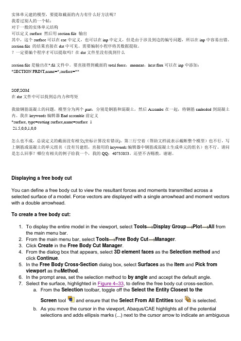
Displaying a free body cutYou can define a free body cut to view the resultant forces and moments transmitted across a selected surface of a model. Force vectors are displayed with a single arrowhead and moment vectors with a double arrowhead.To create a free body cut:1. To display the entire model in the viewport, select Tools Display Group Plot All fromthe main menu bar.2. From the main menu bar, select Tools Free Body Cut Manager.3. Click Create in the Free Body Cut Manager.4. From the dialog box that appears, select 3D element faces as the Selection method andclick Continue.5. In the Free Body Cross-Section dialog box, select Surfaces as the Item and Pick fromviewport as the Method.6. In the prompt area, set the selection method to by angle and accept the default angle.7. Select the surface, highlighted in Figure 4–33, to define the free body cut cross-section.a. From the Selection toolbar, toggle off the Select the Entity Closest to theScreen tool and ensure that the Select From All Entities tool is selected.b. As you move the cursor in the viewport, Abaqus/CAE highlights all of the potentialselections and adds ellipsis marks (...) next to the cursor arrow to indicate an ambiguousselection. Position the cursor so that one of the faces of the desired surface ishighlighted, and click to display the first surface selection.Figure 4–33 Selected faces for the free body cross-section.c. Use the Next and Previous buttons to cycle through the possible selections until theappropriate vertical surface is highlighted, and click OK.8. Click Done in the prompt area to indicate your selection is complete. Click OK in the FreeBody Cross-Section dialog box.9. In the Edit Free Body Cut dialog box, accept the default settings for the SummationPoint and the Component Resolution. Click OK to close the dialog box.10. Click Options in the Free Body Cut Manager.11. From the Free Body Plot Options dialog box, select the Force tab in the Color &Style tabbed page. Click the resultant color sample to change the color of the resultant force arrow.12. Once you have selected a new color for the resultant force arrow, click OK in the Free BodyPlot Options dialog box and click Dismiss in the Free Body Cut Manager.The free body cut is displayed in the viewport, as shown in Figure 4–34.Figure 4–34 Free body cut displayed on the connecting lug.Generating tabular data reports for subsets of the modelTabular output data were generated earlier for this model using printed output requests. However, for complicated models it is convenient to write these data for selected regions of the model using Abaqus/Viewer. This is achieved using display groups in conjunction with the report generation feature. For the connecting lug problem we will generate the following tabular data reports: •Stresses in the elements at the built-in end of the lug (to determine the maximum stress in the lug)•Reaction forces at the built-in end of the lug (to check that the reaction forces at the constraints balance the applied loads)•Vertical displacements at the bottom of the hole (to determine the deflection of the lug when the load is applied)Each of these reports will be generated using display groups whose contents are selected in the viewport. Thus, begin by creating and saving display groups for each region of interest.To create and save a display group containing the elements at the built-in end:1. In the Results Tree, double-click Display Groups.2. Choose Elements from the Item list and Pick from viewport as the selection method.3. Restore the option to select entities closest to the screen.4. In the prompt area, set the selection method to by angle; and click the built-in face of the lug.Click Done when all the elements at the built-in face of the lug are highlighted in the viewport.In the Create Display Group dialog box, click Replace followed by Save As. Save thedisplay group as built-in elements.To create and save a display group containing the nodes at the built-in end:1. In the Create Display Group dialog box, choose Nodes from the Item list and Pick fromviewport as the selection method.2. In the prompt area, set the selection method to by angle; and click the built-in face of the lug.Click Done when all the nodes on the built-in face of the lug are highlighted in the viewport. In the Create Display Group dialog box, click Replace followed by Save As. Save thedisplay group as built-in nodes.To create and save a display group containing the nodes at the bottom of the hole:1. In the Create Display Group dialog box, select All from the item list, and click Replace toreset the active display group to include the entire model.2. In the Create Display Group dialog box, choose Nodes from the Item list and Pick fromviewport as the selection method.3. In the prompt area, set the selection method to individually; and select the nodes at thebottom of the hole in the lug, as indicated in Figure 4–35. Click Done when all the nodes on the bottom of the hole are highlighted in the viewport. In the Create Display Group dialog box,click Replace followed by Save As. Save the display group as nodes at hole bottom.Figure 4–35 Nodes in display group nodes at hole bottom.Now generate the reports.To generate field data reports:1. In the Results Tree, click mouse button 3 on built-in elements underneath the DisplayGroups container. In the menu that appears, select Plot to make it the current display group.2. From the main menu bar, select Report Field Output.3. In the Variable tabbed page of the Report Field Output dialog box, accept the default positionlabeled Integration Point. Click the triangle next to S: Stress components to expand the list of available variables. From this list, select Mises and the six individual stresscomponents: S11, S22, S33, S12, S13, and S23.4. In the Setup tabbed page, name the report Lug.rpt. In the Data region at the bottom of thepage, toggle off Column totals.5. Click Apply.6. In the Results Tree, click mouse button 3 on built-in nodes underneath the DisplayGroups container. In the menu that appears, select Plot to make it the current display group.(To see the nodes, toggle on Show node symbols in the Common Plot Options dialog box.)7. In the Variable tabbed page of the Report Field Output dialog box, change the positionto Unique Nodal. Toggle off S: Stress components, and select RF1, RF2, and RF3 from the list of available RF: Reaction force variables.8. In the Data region at the bottom of the Setup tabbed page, toggle on Column totals.9. Click Apply.10. In the Results Tree, click mouse button 3 on nodes at hole bottom underneath the DisplayGroups container. In the menu that appears, select Plot to make it the current display group.11. In the Variable tabbed page of the Report Field Output dialog box, toggle off RF: Reactionforce, and select U2 from the list of available U: Spatial displacement variables.12. In the Data region at the bottom of the Setup tabbed page, toggle off Column totals.13. Click OK.Open the file Lug.rpt in a text editor. A portion of the table of element stresses is shown below. The element data are given at the element integration points. The integration point associated with a given element is noted under the column labeled Int Pt. The bottom of the table contains information on the maximum and minimum stress values in this group of elements. The results indicate that the maximum Mises stress at the built-in end is approximately 330 MPa. Your results may differ slightly if your mesh is not identical to the one used here.*SECTION PRINTDefine print requests of accumulated quantities on user-defined surface sections.This option is used to provide tabular output of accumulated quantities associated with a user-defined section. Depending on the analysis type the output may include one or several of the following: the total force, the total moment, the total heat flux, the total current, the total mass flow, or the total pore fluid volume flux associated with the section. This option is not available for eigenfrequency extraction, eigenvalue buckling prediction, complex eigenfrequency extraction, or linear dynamics procedures.Product: Abaqus/StandardType: History dataLevel: StepReferences:•“Output to the data and results files,”Section 4.1.2 of the Abaqus Analysis User's Manual •“Abaqus/Standard output variable identifiers,”Section 4.2.1 of the Abaqus Analysis User's ManualRequired parameters:NAMESet this parameter equal to a label that will be used to identify the output for the section. Section names in the same input file must be unique.SURFACESet this parameter equal to the name used in the *SURFACE option to define the surface.Optional parameters:AXESSet AXES=LOCAL if output is desired in the local coordinate system. Set AXES=GLOBAL (default) to output quantities in the global coordinate system.FREQUENCYSet this parameter equal to the output frequency, in increments. The output will always be printed at the last increment of each step unlessFREQUENCY=0. The default is FREQUENCY=1.Set FREQUENCY=0 to suppress the output.UPDATESet UPDATE=NO if output is desired in the original local system of coordinates.Set UPDATE=YES (default) to output quantities in a local system of coordinates that rotates with the average rigid body motion of the surface section. This parameter is relevant only ifAXES=LOCAL and the NLGEOM parameter is active in the step.Optional data lines:First line:1. Node number of the anchor point (blank if coordinates given).2. First coordinate of the anchor point (ignored if node number given).3. Second coordinate of the anchor point (ignored if node number given).4. Third coordinate of the anchor point (for three-dimensional cases only; ignored if node numbergiven).Leave this line blank to allow Abaqus to define the anchor point.Second line:1. Node number used to specify point a in Figure 18.5–1 (blank if coordinates given).2. First coordinate of point a (ignored if node number given).3. Second coordinate of point a (ignored if node number given).The remaining data items are relevant only for three-dimensional cases.4. Third coordinate of point a (ignored if node number given).5. Node number used to specify point b (blank if coordinates given)6. First coordinate of point b (ignored if node number given).7. Second coordinate of point b (ignored if node number given).8. Third coordinate of point b (ignored if node number given).Leave this line blank to allow Abaqus to define the axes.Third line:1. Give the identifying keys for the variables to be output. The keys are defined in the “Sectionvariables” section of “Abaqus/Standard output variable identifiers,”Section 4.2.1 of the Abaqus Analysis User's Manual.Omit both the first and second data lines for AXES=GLOBAL or to allow Abaqus to define the anchor point and the axes for AXES=LOCAL. Repeat the third data line as often as necessary: each line defines a table. If this line is omitted, all appropriate variables (“Output to the data and results files,”Section 4.1.2 of the Abaqus Analysis User's Manual) will be output.Figure 18.5–1 User-defined local coordinate system.SOFTotal force in the section..dat: yes .fil: yes .odb Field: no .odb History: noSOMTotal moment in the section..dat: yes .fil: yes .odb Field: no .odb History: noSOCFCenter of the total force in the section..dat: yes .fil: yes .odb Field: no .odb History: no24.4实体单元的截面力/弯矩/转角[url=/forum/viewthread.php?tid=]/forum/viewthread.php?tid=[/ url]问:求助:请问abaqus里面怎样看一个构件截面(如:钢骨混凝土压弯柱)的内力啊请问:SRC柱模拟后,如何提取截面内力:如某一截面处的轴力、弯矩、剪力等内容,谢谢。
abaqus第二讲:ABAQUS中的实体单元
线性单元 (如:CPS4)
北京怡格明思工程技术有限公司
二次单元 (如:CPS8)
A
9
Innovating through simulation
90o
对于线性完全积分单元,在厚度方向的单元数目并不影响计算结果。误差是由于剪 力自锁(shear locking)引起的,这是存在于所有完全积分、一阶实体单元中的问 题。
壳单元
梁单元
薄膜单元
无限单元
A
北京怡格明思工程技术有限公司
特殊单元,如弹簧、 阻尼器和质量单元
桁架单元
4
Innovating through simulation
ABAQUS中的单元
节点个数 (插值)
• 节点的个数决定了单元的插 值方式。
• ABAQUS包含一阶和二阶插 值方式的单元。
一次插值
二次插值
线性单元 (如:CPS4R)
北京怡格明思工程技术有限公司
二次单元 (如:CPS8R)
A
13
Innovating through simulation
可以通过以下的特征为单元分类: •族 • 节点号 • 自由度 • 公式 • 积分点
A
3
北京怡格明思工程技术有限公司
Innovating through simulation
族
• 有限元族是一种广泛的 分类方法。
• 同族的单元共享许多基 本特征。
• 在同一族单元中又有许 多变异。
连续体(实体单元) 刚体单元
第二讲 ABAQUS中的实体单元
王慎平 北京怡格明思工程技术有限公司
A
1
hrough simulation
ABAQUS中的单元
ABAQUS简支梁分析报告(梁单元和实体单元)
基于ABAQUS简支梁受力和弯矩的相关分析(梁单元和实体单元)对于简支梁,基于 ABAQUS2016,首先用梁单元分析了梁受力作用下的应力,变形,剪力和力矩;对同一模型,并用实体单元进行了相应的分析。
另外,还分析了梁结构受力和弯矩作用下的剪力及力矩分析。
对于CAE仿真分析具体细节操作并没有给出详细的操作,不过在后面上传了对应的cae,odb,inp文件。
不过要注意的是本文采用的是ABAQUS2016进行计算,低版本可能打不开,可以自己提交inp文件自己计算即可。
可以到小木虫搜索:“基于ABAQUS简支梁受力和弯矩的相关分析”进行相应文件下载。
对于一简支梁,其结构简图如下所示,梁的一段受固支,一段受简支,在梁的两端受集中载荷,梁的大直径D=180mm,小直径d=150mm,a=200mm,b=300mm,l=1600mm,F=300000N。
现通过梁单元和实体单元分析简支梁的受力情况,变形情况,以及分析其剪力和弯矩等。
材料采用45#钢,弹性模量E=2.1e6MPa,泊松比v=0.28。
图1 简支梁结构简图1.梁单元分析ABAQUS2016中对应的文件为beam-shaft.cae ,beam-shaft.odb,beam-shaft.inp。
在建立梁part的时候,采用三维线性实体,按照图1所示尺寸建立,然后在台阶及支撑梁处进行分割,结果如图2所示。
图2 建立part并分割接下来为梁结构分配材料,创建材料,定义弹性模量和泊松比,创建梁截面形状,如图3,非别定义两个圆,圆的直接分别为180和150mm。
然后创建两个截面,截面选择梁截面,再选择图2中的所有梁,定义梁的方向矢量为(0,0,-1)(点击图3中的n2,n1,t那个图标即可创建梁的方向矢量),最后把创建好的梁赋给梁结构。
图3 创建梁截面形状接下来装配实体,再创建分析步,在创建分析步的时候,点击主菜单栏的Output,编辑Edit Field Output Request,在SF前面打钩,这样就可以在结果后处理中输出截面剪力和力矩,如图4所示。
abaqus输出文件fil-dat-刚度矩阵等关键词及相关例子
输出 fil文件关键词*Output, history, variable=PRESELECT, time interval=*El file, frequency=999*Node file, frequency=999*El fileS,e*Node fileCF, TF, Ufrequency=1 表示每一个时间增量步输出一次 frequency=999 表示每999个时间增量步输出一次当frequency值足够大时,只在分析步的末端结束时输出数据输出dat文件关键词*Output, history, variable=PRESELECT, time interval=*El print, frequency=999*Node print, frequency=999*El printS11,e11*Node printCF, TF, UEl print El file 将单元上的分析结果(应力、应变和截面力等输出)Node file Node print 将单元上的分析结果(位移、反力输出)输出单元刚度矩阵的方法!*Element Matrix Output,Elset=All, frequency=nFile Name=user defined, file name= abc, Stiffness=Yes mass=yes,DLOAD=YESfrequency=n 每隔n个增量步输出一次单元矩阵,Elset=All all为单元集合名称集合可以在assembly instance中进行定义Stiffness=Yes 表示输出刚度矩阵的的算子矩阵 mass=yes 表示输出质量矩阵DLOAD=YES 表示输出载荷向量no表示输出输出单元刚度矩阵的最终正确方法!*File Format,Ascii*Element Matrix Output,Elset=E1,File Name=abc,Frequency=50,Output File=User Defined,Stiffness=YesE:\xch-cae-nsoft\jiedianli-yanjiu\ 生成文件.mtx所在路径输出单元刚度矩阵的方法!1.用命令:*ELEMENT MATRIX OUTPUT只设定Required parameter:ELSET的话,由于结果文件(*.fil)是二进制文件,用文本编辑器打开是一堆我们看不明白的乱码,所以有必要设置一下文件格式。
- 1、下载文档前请自行甄别文档内容的完整性,平台不提供额外的编辑、内容补充、找答案等附加服务。
- 2、"仅部分预览"的文档,不可在线预览部分如存在完整性等问题,可反馈申请退款(可完整预览的文档不适用该条件!)。
- 3、如文档侵犯您的权益,请联系客服反馈,我们会尽快为您处理(人工客服工作时间:9:00-18:30)。
A B A Q U S实体单元内力
输出
-CAL-FENGHAI-(2020YEAR-YICAI)_JINGBIAN
ABAQUS实体单元弯矩和剪力的输出
闲话少说,直奔主题1.用 free body cut 来做!
1.1在assembly里面做切面分割单元和面的set
在定义了datum面之后,在进行切割时候要将实体变成independent,如上如。
这不操作之后在mesh模块中划分网格不在是part而是assembly来划分网格。
1.2.定义SET
做好切面之后采用下图的方式来进行不断的定义单元和截面,注意是单元和截面,截面时在单元之中的。
1.3.运行free body cut
先是选择定义的单元,然后选择定义的截面!就可以了
1.4.也可以直接选择单元和节点
首先选择的是节点所依附的单元
然后是选择节点
点击 ok
输出的是有弯矩和没有弯矩时候的分量结果。
可以多定义截个这样的free body cut 然后输出
注意:该种方法可以看任何单元的节点的内力值,不一定是一个截面上的!
2.采用view cut来做(简单)
3.Free body cut和view cut共同来做
上述的图加上截面的选取进行定义截面
注意:view cut的剪力正确,弯矩有偏差。
Free body cut相反。
但是划分的单元越小,距离真实值就越近!
free body cut 中的 view cut来进行输出弯矩,轴力和剪力1. 打开 free body cut 创建方式为based on view cut
2.找到了一个view cut ———allow for multiple cuts———copy
3.结果显示如下:
4.report———free body cut
5,打开文件(上面的名字是可以修改的在view cut session 中)6.如果在显示中要打开moment,可以free body cut manager设置。