SPTK 3.3 examples

合集下载

SPAS 2023.3.31版 Strati

Package‘SPAS’April21,2023Type PackageTitle Stratiﬁed-Petersen Analysis SystemVersion2023.3.31Date2023-03-31Author Carl James SchwarzMaintainer Carl James Schwarz<******************************>LinkingTo TMB,RcppEigenImports MASS,Matrix,msm,numDeriv,plyr,reshape2,TMB(>=1.7.15)Description The Stratiﬁed-Petersen Analysis System(SPAS)is designedto estimate abundance in two-sample capture-recapture experimentswhere the capture and recaptures are stratiﬁed.This is a generalizationof the simple Lincoln-Petersen estimator.Strata may be deﬁned in time or in space or both,and the s strata in which marking takes placemay differ from the t strata in which recoveries take place.When s=t,SPAS reduces to the method described byDarroch(1961)<https:///stable/2332748>.When s<t,SPAS implements the methods described inPlante,Rivest,and Tremblay(1988)<https:///stable/2533994>.Schwarz and Taylor(1998)<https:///doi/10.1139/f97-238>describe the use of SPAS in estimating return of salmon stratiﬁed bytime and geography.A related package,BTSPAS,deals with temporal stratiﬁcation wherea spline is used to model the distribution of the populationover time as it passes the second capture location.This is the R-version of the(now obsolete)standalone Windowsprogram available at<https://home.cs.umanitoba.ca/~popan/spas/spas_home.html>. License GPL(>=2)RoxygenNote7.2.3Suggests knitr,rmarkdownVignetteBuilder knitrEncoding UTF-81NeedsCompilation yesRepository CRANDate/Publication2023-04-2022:12:40UTCR topics documented:SPAS.autopool (2)SPAS.ﬁt.model (4)SPAS.print.model (6)Index7 SPAS.autopool Autopooling a Stratiﬁed-Petersen(SP)data set.This function appliespooling rules to pool a SPAS dataset to meeting minimum sparsityrequirements.DescriptionAutopooling a Stratiﬁed-Petersen(SP)data set.This function applies pooling rules to pool a SPAS dataset to meeting minimum sparsity requirements.UsageSPAS.autopool(rawdata,min.released=100,min.inspected=50,min.recaps=50,min.rows=1,min.cols=1)Argumentsrawdata An(s+1)x(t+1)of the raw data BEFORE pooling.The s x t upper left matrix is the number of animals released in row stratum i and recovered in column stratumj.Row s+1contains the total number of UNMARKED animals recovered incolumn stratum j.Column t+1contains the number of animals marked in eachrow stratum but not recovered in any column stratum.The rawdata[s+1,t+1]isnot used and can be set to0or NA.The sum of the entries in each of theﬁrsts rows is then the number of animals marked in each row stratum.The sum ofthe entries in each of theﬁrst t columns is then the number of animals captured(marked and unmarked)in each column stratum.The row/column names of thematrix may be set to identify the entries in the output.min.released Minimum number of releases in a pooled rowmin.inspected Minimum number of inspections in a pooled columnmin.recaps Minimum number of recaptures before any rows can be pooledmin.rows,min.colsMinimum number or rows and columns after poolingDetailsIn many cases,the stratiﬁed set of releases and recapture is too sparse(many zeroes)or count are very small.Pooling rows and columns may be needed.Data needs to be pooled both row wise and column wise if the data are sparse to avoid singularities in theﬁt.This function automates pooling rows or columns following Schwarz and Taylor(1998).•All rows that have0releases are discarded•All columns that have0recaptures of taggedﬁsh and0ﬁsh inspected are discarded•Starting at theﬁrst row and working forwards in time,and then working from theﬁnal rowand working backwards in time,.rows are pooled until a minimum of min.released arereleased.An alternating pooling(from the top,from the bottom,from the top,etc)is used•Starting at theﬁrst column and working forwards in time,.and then working from theﬁnalcolumn and working backwards in time,columns are pooled until a minimum of min.inspected are inspected.An alternating pooling(from the left,from the right,from the left,etc)is used.•If the sum of the total recaptures from releasedﬁsh is<=min.recaps,then all rows are pooled(which reduces to a Chapman estimator)ValueA list with a suggest pooling.Examplesconne.data.csv<-textConnection("9,21,0,0,0,0,1710,101,22,1,0,0,7630,0,128,49,0,0,9340,0,0,48,12,0,4340,0,0,0,7,0,490,0,0,0,0,0,4351,2736,3847,1818,543,191,0")conne.data<-as.matrix(read.csv(conne.data.csv,header=FALSE))close(conne.data.csv)SPAS.autopool(conne.data)SPAS.fit.model Fit a Stratiﬁed-Petersen(SP)model using TMB.DescriptionThis functionﬁts a Stratiﬁed-Petersen(Plante,1996)to data and specify which rows/columns of the data should be pooled.The number of rows after pooling should be<=number of columns after pooling.UsageSPAS.fit.model(model.id="Stratified Petersen Estimator",rawdata,autopool=FALSE,row.pool.in=NULL,col.pool.in=NULL,row.physical.pool=TRUE,theta.pool=FALSE,CJSpool=FALSE,optMethod=c("nlminb"),optMethod.control=list(maxit=50000),svd.cutoff=1e-04,chisq.cutoff=0.1,min.released=100,min.inspected=50,min.recaps=50,min.rows=1,min.cols=1)Argumentsmodel.id Character string identifying the name of the model including any pooling..rawdata An(s+1)x(t+1)of the raw data BEFORE pooling.The s x t upper left matrix is the number of animals released in row stratum i and recovered in column stratumj.Row s+1contains the total number of UNMARKED animals recovered incolumn stratum j.Column t+1contains the number of animals marked in eachrow stratum but not recovered in any column stratum.The rawdata[s+1,t+1]isnot used and can be set to0or NA.The sum of the entries in each of theﬁrsts rows is then the number of animals marked in each row stratum.The sum ofthe entries in each of theﬁrst t columns is then the number of animals captured(marked and unmarked)in each column stratum.The row/column names of thematrix may be set to identify the entries in the output.autopool Should the automatic pooling algorithms be used.Give more details here on these rule work.row.pool.in,col.pool.inVectors(character/numeric)of length s and t respectively.These identify therows/columns to be pooled before the analysis is done.The vectors consists ofentries where pooling takes place if the entries are the same.For example,if s=4,then row.pool.in=c(1,2,3,4)implies no pooling because all entries are distinct;row.pool.in=c("a","a","b","b")implies that theﬁrst two rows will be pooled andthe last two rows will be pooled.It is not necessary that row/columns be contin-uous to be pooled,but this is seldom sensible.A careful choice of pooling labelshelps to remember what as done,e.g.row.pool.in=c("123","123","123","4")in-dicates that theﬁrst3rows are pooled and the4th row is not pooled.Characterentries ensure that the resulting matrix is sorted properly(e.g.if row.pool.in=c(123,123,123,4),then the same pooling is done,but the matrix rows are sorted rather strangely.row.physical.poolShould physical pooling be done(default)or should logical pooling be done.Forexample,if there are3rows in the data matrix and row.pool.in=c(1,1,3),then inphysical pooling,the entries in rows1and2are physically added together tocreate2rows in the data matrix beforeﬁtting.Because the data has changed,you cannot compare physical pooling using AIC.In logical pooling,the datamatrix is unchanged,but now parameters p1=p2but the movement parametersfor the rest of the matrix are not forced equal.theta.pool,CJSpoolNOT YET IMPLEMENTED.DO NOT CHANGE.optMethod What optimization method is used.Defaults is the nlminb()function..optMethod.controlControl parameters for optimization method.See the documentation on the dif-ferent optimization methods for details.svd.cutoff Whenﬁnding the variance-covariance matrix,a singular value decomposition isused.This identiﬁes the smallest singular value to retain.chisq.cutoff Whenﬁnding a goodness ofﬁt statistic using(obs-exp)^2/exp,all cell whoseExp<gof.cutoff are ignored to try and remove structural zero cells.min.released Minimum number of releases in a pooled rowmin.inspected Minimum number of inspections in a pooled columnmin.recaps Minimum number of recaptures before any rows can be pooledmin.rows,min.colsMinimum number or rows and columns after poolingValueA list with many entries.Refer to the vignettes for more details.Examplesconne.data.csv<-textConnection("9,21,0,0,0,0,1710,101,22,1,0,0,7630,0,128,49,0,0,9340,0,0,48,12,0,4346SPAS.print.model 0,0,0,0,7,0,490,0,0,0,0,0,4351,2736,3847,1818,543,191,0")conne.data<-as.matrix(read.csv(conne.data.csv,header=FALSE))close(conne.data.csv)mod1<-SPAS.fit.model(conne.data,model.id="Pooling rows1/2,5/6;pooling columns5/6",row.pool.in=c("12","12","3","4","56","56"),col.pool.in=c(1,2,3,4,56,56))mod2<-SPAS.fit.model(conne.data,model.id="Auto pool",autopool=TRUE)SPAS.print.model Print the results from aﬁt of a Stratiﬁed-Petersen(SP)model whenusing the TMB optimizerDescriptionThis function makes a report of the results of the modelﬁtting.UsageSPAS.print.model(x)Argumentsx A result from the modelﬁtting.See SPAS.fit.model.ValueA report to the console.Refer to the vignettes.Examplesconne.data.csv<-textConnection("9,21,0,0,0,0,1710,101,22,1,0,0,7630,0,128,49,0,0,9340,0,0,48,12,0,4340,0,0,0,7,0,490,0,0,0,0,0,4351,2736,3847,1818,543,191,0")conne.data<-as.matrix(read.csv(conne.data.csv,header=FALSE))close(conne.data.csv)mod1<-SPAS.fit.model(conne.data,model.id="Pooling rows1/2,5/6;pooling columns5/6",row.pool.in=c("12","12","3","4","56","56"),col.pool.in=c(1,2,3,4,56,56))SPAS.print.model(mod1)IndexSPAS.autopool,2SPAS.fit.model,4SPAS.print.model,67。

Onpattro (patisiran lipid complex) 泛型说明文档说明书

Onpattro (patisiran lipid complex)(Intravenous)Document Number: IC-0379 Last Review Date: 10/01/2019Date of Origin: 09/05/2018Dates Reviewed: 09/2018, 10/2019I.Length of AuthorizationCoverage will be provided for six months and may be renewed.II.Dosing LimitsA.Quantity Limit (max daily dose) [Pharmacy Benefit]:∙Onpattro 10 mg injection: 3 vials every 3 weeksB.Max Units (per dose and over time) [Medical Benefit]:∙300 billable units every 3 weeksIII.Initial Approval CriteriaCoverage is provided in the following conditions:∙Must not be used in combination with other transthyretin (TTR) reducing agents (e.g., inotersen, tafamidis, etc.); ANDPolyneuropathy due to Hereditary Transthyretin-Mediated (hATTR) Amyloidosis /FamilialAmyloidotic Polyneuropathy (FAP) †∙Patient must be at least 18 years old; AND∙Patient has a definitive diagnosis of hATTR amyloidosis/FAP as documented by amyloid deposition on tissue biopsy and identification of a pathogenic TTR variant using moleculargenetic testing; AND∙Used for the treatment of polyneuropathy as demonstrated by at least TWO of the following criteria:o Subjective patient symptoms are suggestive of neuropathyo Abnormal nerve conduction studies are consistent with polyneuropathyo Abnormal neurological examination is suggestive of neuropathy; AND∙Patient’s peripheral neuropathy is attributed to hATTR/FAP and other causes of neuropathy have been excluded; AND∙Baseline in strength/weakness has been documented using an objective clinical measuring tool (e.g., Medical Research Council (MRC) muscle strength, etc.); AND∙Patient has not been the recipient of an orthotopic liver transplant (OLT); AND∙Patient is receiving supplementation with vitamin A at the recommended daily allowance †FDA Approved Indication(s); ‡ Compendium Recommended Indication(s)IV.Renewal CriteriaAuthorizations can be renewed based on the following criteria:∙Patient continues to meet the criteria identified in section III; AND∙Absence of unacceptable toxicity from the drug. Examples of unacceptable toxicity include the following: severe infusion-related reactions, ocular symptoms related tohypovitaminosis A, etc.; AND∙Disease response compared to pre-treatment baseline as evidenced by stabilization or improvement in one or more of the following:o Signs and symptoms of neuropathyo MRC muscle strengthV.Dosage/AdministrationVI.Billing Code/Availability InformationHCPCS code:∙J0222 - Injection, patisiran, 0.1 mg; 1 billable unit = 0.1 mgNDC:Onpattro 10 mg/5 mL single-dose vial: 71336-1000-xxVII.References1.Onpattro [package insert]. Cambridge, MA; Alnylam Pharmaceuticals, Inc., August 2018.Accessed August 2019.2.Adams D, Gonzalez-Duarte A, O’Riordan WD, et al. Patisiran, an RNAi Therapeutic, forHereditary Transthyretin Amyloidosis. N Engl J Med. 2018 Jul 5;379(1):11-21. doi:10.1056/NEJMoa17161533.Adams D, Suhr OB, Dyck PJ, et al. Trial design and rationale for APOLLO, a Phase 3,placebo-controlled study of patisiran in patients with hereditary ATTR amyloidosis withpolyneuropathy. BMC Neurol. 2017;17(1):1814.Sekijima Y, Yoshida K, Tokuda T, et al. Familial Transthyretin Amyloidosis. Gene Reviews.Adam MP, Ardinger HH, Pagon RA, et al., editors. Seattle (WA): University of Washington,Seattle; 1993-2018.5.Ando Y, Coelho T, Berk JL, et al. Guideline of transthyretin-related hereditary amyloidosisfor clinicians. Orphanet J Rare Dis. 2013;8:31.Appendix 1 – Covered Diagnosis CodesAppendix 2 – Centers for Medicare and Medicaid Services (CMS)Medicare coverage for outpatient (Part B) drugs is outlined in the Medicare Benefit Policy Manual (Pub. 100-2), Chapter 15, §50 Drugs and Biologicals. In addition, National CoverageDetermination (NCD) and Local Coverage Determinations (LCDs) may exist and compliance with these policies is required where applicable. They can be found at: /medicare-coverage-database/search/advanced-search.aspx. Additional indications may be covered at the discretion of the health plan.Medicare Part B Covered Diagnosis Codes (applicable to existing NCD/LCD): N/A。

kisssoft-anl-003-E-din743-intro

KISSsoft, shaft analysis:Introduction to DIN 743, October 2000Shafts and axles, calculation of load capacityIntroductionPurposeThe DIN 743 for strength analysis of shafts and axles is a most helpful analysis method available in the KISSsoft software, [1], for analysis of machine elements. The standard however is available in German only and the theory behind the software KISSsoft is not readily available for non german speaking customers. Therefore, a short introduction to the said standard is given herewith. The DIN 743 The German standard DIN 743 [2] has been prepared by the German institute for standardisation and the Institut für Maschinenelemente und Maschinenkonstruktion of the technical university of Dresden, Germany. The objective was to make available for the engineering community a standard focusing on strength analysis of shafts and axles. The standard is based on the standard TGL 19340 of the former German Democratic Republic, the VDI 2226 of the Federal Republic of Germany and the FKMguideline compiled by the IMA Dresden, Germany, see [3], [4], [13]. The proof of strength is based on the calculation of a safety factor against fatigue and against static failure. The safety factors have to be higher than a required minimal safety factor. If this condition is fulfilled, proof is delivered. The standard consists of four parts:Part 1: Introduction, analysis methodPart 2: Stress concentration factors and fatigue notch factorsPart 3: Materials dataPart 4: ExamplesLimitationsThe analytical proof considers bending, tensile/compressive and shear stresses due to torsion.However, shear stresses due to shear forces are not considered, hence use of this standard for short shafts requires caution.Only the fatigue limit is used in the proof, no proof for finite life strength is delivered. However, an extension is planned, see section 0.Materials data are based on 107 stress cycles with a probability of survival of 97.5%.The safety factor required in the standard covers only the uncertainty in the analysis procedure.Additional safety factors or an increased safety factor due to uncertainties in the load assumptions and due to the effects of a failure are not defined. They have to be defined by the engineer.I n t r o d u c t i o n t o D I N 743The notch factors for feather keys are questionable since no difference is made for the different key forms.All loads (bending, tensile/compression, shear) are in phase.The standard does not cover the calculation of the load acting.The standard is limited to non-welded steels in the range of –40C ° to 150C °. The environment has to be non-corrosive for application of this standard.LoadsThe loads acting on the part are defined by describing the effective load amplitudes and the mean loads (for the fatigue proof) and the maximum acting load (for static proof). These loads are to be calculated according to the nominal stress concept, using standard engineering formulas.Proof against fatigue failure SafetyIn order to deliver the proof against fatigue failure, the safety S calculated has to be higher than the minimal required safety S min . According to the standard, S min has to be at least 1.2. Uncertainties in the load assumptions and severe effects in case of failure require higher safety factors, to be defined by the engineer. The safety S is calculated from partial safeties according to the following formula: 221⎟⎟⎠⎞⎜⎜⎝⎛+⎟⎟⎠⎞⎜⎜⎝⎛+=tADK ta bADK ba zdADK zda S ττσσσσwhereta ba zda τσσ,, Stress amplitudes due to tension/compression, bending, torsiontADK bADK zdADK τσσ,, Permissible stress amplitudes, strengthsThe form of the above formula is based on the idea of partial safeties for the specific load types (normal stresses / shear stresses) combined in elliptic form.The stress amplitudes are calculated based on the nominal stress concept, considering the cross section of the shaft (A, I, W b , W p ) and external loads (moments, forces).For calculation of the permissible stress amplitudes, see section 0.Condition for delivery of proof is that20.1min ≥≥S STwo different cases are distinguished:Case 1: The safety factor is based only on the comparison between actual and permissible stress amplitude, leaving the mean stress on a constant levelCase 2: The safety is based on the assumption that the stress ratio used for calculation of permissible stress amplitude is equal to the stress ratio as it is for the actual stress amplitudeThe latter is the more conservative approach and recommended.Strength of the partThe strength of the part (index ADK) is being calculated from the strength of the un-notched material specimen. It is a nominal stress considering- Technological size factor K 1(d eff ): effect of heat treatment (size of shaft), depending on diameter at time of treatment), see section 0- Geometrical size factor K 2(d): effect of stress gradient on bending strength compared to tensilestrength of specimen, see section 0- Notches, notch factor βσ(d), βτ(d): effect of local stress increasers/notches- Surface roughness factor K F σ, K F τ, see section 0- Surface hardening factor K V : effect of compressive residual stresses, see section 0Mean stress sensitivity ψσK and ψτK : Effect of mean stress level on permissible stress amplitude.Basic assumption is that the ultimate strength R m or σB is based on a reference diameter d B for which the ultimate strength R m is tabulated (see part 3 of the standard).R m / σB may also be estimated from measured Brinell hardness values according to:HB B H *3.0≈σFor a part with diameter d>d B lower strength applies, the difference being considered using the technological size factor K 1(d). This factor depends on the type of material used and its hardenability / heat treatability:)(*)()(1B B B d d K d σσ=WhereσzB (d)Strength of the part with diameter dσzB (d B ) Strength of the specimen with diameter d BK 1(d) Technological size coefficientBased on this ultimate strength of the part, the fatigue strengths are estimated as follows (for bending, tension/compression and shear):)(*3.0)()(*4.0)()(*5.0)(d d d d d d B tw B zdw B bw στσσσσ===The fatigue strength of the notched part then is (influence of mean stress not yet considered, see section 0), for tension/compression (index zd), bending (index b) and torsion (index t):τσσττσσσσK d K d K d K d K d K d eff B tW tWK eff B bW bWK eff B zdW zdWK )(*)()(*)()(*)(111===WhereK 1(d eff )Technological size factortW bW zdW τσσ,, Strength of the un-notched specimen with diameter d B These values are listed in Part 3 of the standardV F V F K K d K K K K d K K 1*11)(1*11)(22⎟⎟⎠⎞⎜⎜⎝⎛−+=⎟⎟⎠⎞⎜⎜⎝⎛−+=τττσσσββWhereK 2(d) Geometrical size coefficient, see section 0βσ,τNotch factor for compression/tension, bending and torsion Listed in Part 2 of the standardHence, the effect of the notch is considered in the permissible stress and not in the actual stress (calculated as nominal stress). Influence of mean stressTwo different cases are to be distinguished, see case 1 and case 2 in section 0. In both cases, thestrength of the notched part considering the mean stress is a function of the strength of the notched part not considering the mean stress, the mean stress and the mean stress sensitivity:),,,,,,,(,,K K b K zd mv mv tWK bWK zdWK tADK bADK zdADK f τσσψψψτστσστσσ=For case 1, we find:mvK tWK zdADK mv K b bWK bADK mvK zd zdWK zdADK τψτσσψσσσψσστσσ***−=−=−=And for case 2 (limiting conditions not shown, see standard for more details)ta mvK tWK tADK bamvK b bWKbADK zdamvK zd zdWKzdADK a ττψττσσψσσσσψσστσσ**1*1+=+=+=Where()3*322mvmv tmbm zdm mv σττσσσ=++=The mean stress sensitivity factors ψ themselves depend on the ultimate strength of the material and the alternating strength. According to the formulas used in the standard, the mean stress sensitivity factor is independent of the level of the mean stress, although new findings show that it is higher for low mean stresses and lower for higher mean stresses, see [11].Static proofSafetyFor this proof, the maximum stress occurring during the lifetime of the part is to be compared to it’s strength. The resulting safety is calculated as follows:2max 2max max 1⎟⎟⎠⎞⎜⎜⎝⎛+⎟⎟⎠⎞⎜⎜⎝⎛+=tFK t bFK b zdFK zd S ττσσσσNote that for the static proof, the effect of notches is not considered.Strength of the partIn the above formula, strengths of the part (in the denominators) are compared to the acting stresses (in the numerators). The comparisons are than added up in the sense of a elliptic safety criterion.Generally, the yield strength of the part of diameter d is not known (e.g. from measurement) and is to be estimated from the values of the specimen with diameter d B . The yield strengths of the part, generally written as σs (d) (yield strength for a part of diameter d) are calculated as follws:3/)(***)()(***)()(***)(212121B s F F eff tFK B s F F eff bFK B s F F eff zdFK d K d K d K d K d K d K σγτσγσσγσ===Where- K 1(d eff ) is the technological size coefficient- K 2F is the static support coefficient depending on the presence of a hardened outer layer of the material- γF is a coefficient for increasing the yield strength due to a multi-axial stress state in a notch - σS (d B ) is the yield strength of the specimen with diameter d BRemarks Notch effectsThe notch factor β is defined through the permissible stress amplitude against fatigue failure of the un-notched specimen of diameter d compared to the one of the notched part:tWK tW bWKzd bW zd d d ττβσσβτσ)()(,,==Whereas the form factor α is the coefficient of the stress value in the notch compared to the stress value in the un-disturbed cross section (nominal stress). Hence, whereas the form factor is a function only of the geometry of the part, the notch factor β is also a function of the material and the stress state. The notch factor β can be calculated from the form factor α as follows:n τστσαβ,,=Where n is the support coefficient to be calculated from the materials strength and the stress gradient in the notch. The stress gradient can either be calculated by means of FEM or estimated through formulas given in the standard.Different notch factors are given for all three load types considered (bending, tension/compression and torsion), Influence of sizeThe influence of the size of a part on it’s strength is to be considered in three factors:1) Technological size coefficient K 1(d eff ): With this factor the fact that the effect of hardening / heat treatment and hence the strength is reduced with increasing part diameter. This coefficient is independent of the type of load (tension/compression, bending, shear). The coefficient is to be estimated using the effective diameter during heat treatment. The coefficient is to beconsidered if the strength of the part is not measured but calculated from the strength of the specimen as tabulated in the standard.2) Geometrical size coefficient K 2(d): With this factor, the effect that the strength against bending converges towards the strength against tension/compression with increasing part diameter andthat the strength against shear due to torsion is also being reduced. This is due to the decreasing stress gradient with increasing part diameter. With the decreasing stress gradient, the support coefficient n also decreases.3) Geometrical size coefficient K 3(d): Same effect as in 2) but here for the notched part.Influence of surface hardeningWith the coefficient K V effects due to surface hardening depending on the procedure applied areconsidered. The underlying effects covered are the surface hardness and induced compressive stresses. It is recommended to use the lower range of the tabulated values or to conduct experiments if the higher values are to be used, see for example [6].Finite life calculationThe standard DIN 743 covers only the proof against fatigue failure for infinite life. However, anextension to finite life calculation is planned, see [12], [8]. With this extension, load spectrums can be considered. Based on the load spectrum, a damage equivalent load is calculated. Based on this damage equivalent load, using a S-N curve, the lifetime is estimated or the proof for infinite life is delivered.The damage equivalent load amplitude is calculated as follows:koll a a f /1σσ=Whereσa is the damage equivalent load amplitudeσa1 is the highest load amplitude of the collectivef koll describes the shape of the load sepctrum, calculated according to different variations of Miners rule, see [12]The permissible stress amplitude for a required life time is calculated as follows:ADK q LD ANK N N σσ*=WhereσANK is the permissible stress amplitude for finite lifeσADK is the permissible stress amplitude for infinite lifeN D = 1*106 cyclesN L is the required life (cycles), 1*103<N L <N Dq=5 for bending and tension/compression, q=8 for torsion Comparison to other analysis methodsIn [7], [9] and [5], comparisons of the analysis method according to DIN 743 with other methods, FKM-Richtlinie [13], Nieman [14] and Hänchen + Decker [15], are described.In comparison with the FKM-guideline, the following differences are found:- In the FKM guideline, shear stress due to shear forces are considered- The minimal safety factors required also depend on the material, load assumptions and effect of failure-High temperature is considered in static proof-Differences in notch factorsA comparison with the other two methods cited shows that the complete analysis procedure is quite different.All authors agree that the deviations in the results strongly depend on the notch considered. No clear tendencies were found when comparing the results, but the usefulness of the standard and the soundness of the design resulting from its use were confirmed in all cases.References[1]KISSsoft Software, Calculation software for machine design, www.KISSsoft.ch[2]DIN 743, Teile 1-3, Tragfähigkeitsberechnung von Wellen und Achsen, 2000[3]TGL 19340, Dauerfestigkeit der Maschinenbauteile, März 1983[4]VDI Richtlinie 2226, Empfehlung für die Festigkeitsberechnung metallischer Bauteile, VDI-Verlag, 1965[5] B. Schlecht, Vergleichende Betrachtungen zum Tragfähigkeitsnachweis der Wellen in Sondergetriebenvon Tagebaugrossgeräten, VDI Berichte Nr. 1442, 1998[6]T. Körner, H. Depping, J. Häckh, G. Willmerding, W. Klos, Rechnerische Lebensdauerabschätzung unterBerücksichtigung realer Belastungskollektive für die Hauptwelle eines Nutzfahrzeuggetriebes, VDIBerichte Nr. 1689, 2002[7]M. Bachmann, Anwendung der DIN 743 in der Antriebstechnik, VDI Berichte Nr. 1442, 1998[8]H. Linke, Praxisorientierte Berechnung von Wellen und Achsen nach DIN 743, VDI Berichte 1442, 1998[9]U. Kissling, Festigkeitsberechnung von Wellen – Einführung von neuen Normen, internal report,KISSsoft AG[10]U. Kissling, Festigkeitsberechnung von Wellen und Achsen nach neuen Normen, Antriebstechnik 36 Nr.10, 1997[11]H. Linke, I. Römhild, Belastbarkeit von Wellen und Achsen nach DIN 743, VDI/EKV Tagung Welle-Nabe-Verbindungen, April 1998, Fulda[12]Entwurf Berechnungsvorschlag FVA – BV 743, Tragfähigkeitsberechnung von Achsen und Wellen,Ergänzung zu DIN 743, Erfassung von Lastkollektiven und Berechnungen der Sicherheit im Dauer- und Zeitfestigkeitsbereich[13]FKM-Richtlinie 154, Rechnerischer Festigkeitsnachweis für Maschinenbauteile[14]G. Niemann, Maschinenelemente, Band 1, Springer 1981[15]R. Hänchen, K.-H. Decker, Neue Festigkeitslehre für den Maschinenbau, 2.te Auflage, Carl HanserVerlag, 1967.。

用php写whatsapp发送模板的范文

用php写whatsapp发送模板的范文下载提示：该文档是本店铺精心编制而成的，希望大家下载后，能够帮助大家解决实际问题。

文档下载后可定制修改，请根据实际需要进行调整和使用，谢谢!本店铺为大家提供各种类型的实用资料，如教育随笔、日记赏析、句子摘抄、古诗大全、经典美文、话题作文、工作总结、词语解析、文案摘录、其他资料等等，想了解不同资料格式和写法，敬请关注!Download tips: This document is carefully compiled by this editor. I hope that after you download it, it can help you solve practical problems. The document can be customized and modified after downloading, please adjust and use it according to actual needs, thank you! In addition, this shop provides you with various types of practical materials, such as educational essays, diary appreciation, sentence excerpts, ancient poems, classic articles, topic composition, work summary, word parsing, copy excerpts, other materials and so on, want to know different data formats and writing methods, please pay attention!在当今社会，随着智能手机的普及和即时通讯工具的飞速发展，WhatsApp已经成为了人们日常生活中不可或缺的一部分。

CMMI ML3 最新访谈问题集 for EPG_QA

文档审计工作是如何开展的？
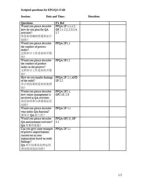
PPQA SP1.2
How do you handle findings of the audit?
审计的结果你是如何处理的？
PPQA SP 2.1 AND SP 2.2
Would you please describe how senior management is involved in QA activities
and all PAs GP 2.8/3.2
Would you please describe how do you communicate and use measurement results?
你怎样交流和利用度量结果的？
MA SP 2.4
Can you give examples of process improvements carried out based on data analysis
Scripted questions for EPG/QA FAR
Session:Date and Time:Duration:
Questions
PA Ref
Would you please describe how do you plan for QA activities?
你是如何编制质量保证计划的？
过程是怎样被评价的？
OPF SP 1.2
Would you please describe how do you establish and implement process action items?
怎样建立和实施过程改进项的？
OPF SP 2.1 and 2.2
Would you please describe how process training are carried out in your organization

磷脂酰肌醇3激酶β(PI3Kβ)和PI3Kδ在KIT突变介导的细胞转化中起不同作用

细胞与分子免疫学杂志（Chin J Cell Mollmmunol)2021，37( 1)39•论著•文章编号：1007-8738(2021 )01>0039~08磷脂酰肌醇3激酶p(PI3Kp)和PI3K8在K IT突变介导的细胞转化中起不同作用张少婷，朱光荣，石君，杨继辉，蒋宗英，张良颖，窦凯凯，孙建民*(宁夏医科大学基础医学院病原生物学与医学免疫学系，宁夏银川750004)[摘要]目的探究磷脂酰肌醇3激酶(P I3K)的不同亚型在三型酪氨酸激酶受体KIT突变介导的信号传递及细胞增殖中的作用。

方法在B aF3细胞中稳定表达野生型KIT及胃肠间质瘤中常见的KIT突变V560D、W557K558del,分别用PI3K a、P I3KP、P I3K5亚型特异性抑制剂或者广谱P I3K抑制剂处理细胞，免疫沉淀法和W estern blot法检测KIT及其下游信号活化情况。

胃肠间质瘤G IST-T1细胞采用相同药物及浓度处理，免疫共沉淀和W estern blot法检测KIT及其下游信号的活化情况，噻唑蓝 (M T T)法检测细胞增殖，流式细胞术检测细胞凋亡。

结果与对照组相比，在表达野生型KIT及其突变体的B aF3细胞中，P I3K8亚型特异性抑制剂对KIT及其下游信号分子蛋白激酶B(AKT)和胞外信号调节激酶（ERK)活化的抑制作用最强，其次为 P I3K a和P I3KP亚型特异性抑制剂。

在G IST-T1细胞中，P I3KP亚型特异性抑制剂对KJT及其下游信号活化的抑制作用最强,其次为P I3K&和P I3K a亚型特异性抑制剂。

结论在B aF3细胞中，P I3KS亚型在KIT活化及其下游信号传递中起主要作用，而在G IST-T1细胞中，P I3Kp亚型在KIT活化及其下游信号传递中起主要作用，这些结果表明不同P I3K亚型在KIT突变介导的细胞转化中起不同作用，且在不同的细胞中其作用也有不同。

一篇影响因子超40的蛋白组学Protein Analysis by Shotgun Bottom-up Proteomics

† ‡
Department of Chemical Physiology, The Scripps Research Institute, La Jolla, California 92037, United States Department of Molecular Medicine, Cell and Matrix Biology Research Institute, School of Medicine, Kyungpook National University, Daegu 700-422, Republic of Korea
1. INTRODUCTION According to Genome Sequencing Project statistics (http:// /genomes/static/gpstat.html), as of February 16, 2012, complete gene sequences have become available for 2816 viruses, 1117 prokaryotes, and 36 eukaryotes.1,2 The availability of full genome sequences has greatly facilitated biological research in many ﬁelds, including the growth of mass spectrometry-based proteomics. Proteins are important because they are the direct biofunctional molecules in living organisms. The term “proteomics” was coined from merging “protein” and “genomics” in the 1990s.3,4 As a postgenomic discipline, proteomics encompasses eﬀorts to identify and quantify all the proteins of a proteome, including expression, cellular localization, interactions, posttranslational modiﬁcations (PTMs), and turnover as a function of time, space, and cell type, thus making the full investigation of a proteome more challenging than sequencing a genome.

spatstat.Knet 3.0-2 软件包说明说明书

Package‘spatstat.Knet’November13,2022Type PackageTitle Extension to'spatstat'for Large Datasets on a Linear NetworkVersion3.0-2Date2022-11-12Depends R(>=3.5.0),spatstat.data(>=3.0),spatstat.sparse(>=3.0),spatstat.geom(>=3.0),spatstat.random(>=3.0),spatstat.explore,spatstat.model,spatstat.linnet(>=3.0),spatstat(>=3.0)Imports spatstat.utils(>=3.0),MatrixMaintainer Adrian Baddeley<**************************.au>Description Extension to the'spatstat'family of packages,for analysinglarge datasets of spatial points on a network.The geometrically-corrected K function is computed using a memory-efﬁcienttree-based algorithm described by Rakshit,Baddeley and Nair(2019).License GPL(>=2)NeedsCompilation yesByteCompile trueAuthor Suman Rakshit[aut,cph](<https:///0000-0003-0052-128X>), Adrian Baddeley[cre,cph](<https:///0000-0001-9499-8382>)Repository CRANDate/Publication2022-11-1305:40:08UTCR topics documented:spatstat.Knet-package (2)Knet (3)Knetinhom (4)wacrashes (5)Index712spatstat.Knet-packagespatstat.Knet-package Extension to’spatstat’for Large Datasets on a Linear NetworkDescriptionExtension to the’spatstat’family of packages,for analysing large datasets of spatial points on anetwork.The geometrically-corrected K function is computed using a memory-efﬁcient tree-basedalgorithm described by Rakshit,Baddeley and Nair(2019).DetailsThis is an extension to the spatstat package for the analysis of large data sets on linear networks.Its main functionality is a memory-efﬁcient algorithm for computing the estimate of the K functionon a linear network,described in Rakshit et al(2019).The main functions are Knet and Knetinhom.These are counterparts of the functions linearK andlinearKinhom in the spatstat.linnet package.The spatstat.linnet functions linearK and linearKinhom are usable(and slightly faster)for smalldatasets,but require substantial amounts of memory.For larger datasets,the functions Knet andKnetinhom are much more efﬁcient.The DESCRIPTIONﬁle:Package:spatstat.KnetType:PackageTitle:Extension to’spatstat’for Large Datasets on a Linear NetworkVersion: 3.0-2Date:2022-11-12Depends:R(>=3.5.0),spatstat.data(>=3.0),spatstat.sparse(>=3.0),spatstat.geom(>=3.0),spatstat.random(>= Imports:spatstat.utils(>=3.0),MatrixAuthors@R:c(person(given="Suman",family="Rakshit",role=c("aut","cph"),email="************************. Maintainer:Adrian Baddeley<**************************.au>Description:Extension to the’spatstat’family of packages,for analysing large datasets of spatial points on a network License:GPL(>=2)NeedsCompilation:yesByteCompile:trueAuthor:Suman Rakshit[aut,cph](<https:///0000-0003-0052-128X>),Adrian Baddeley[cre,cph](<httIndex of help topics:Knet Geometrically-Corrected K Function on NetworkKnetinhom Geometrically-Corrected Inhomogeneous KFunction on Networkspatstat.Knet-package Extension to spatstat for Large Datasets on aLinear Networkwacrashes Road Accidents in Western AustraliaKnet3Author(s)NAMaintainer:Adrian Baddeley<**************************.au>ReferencesRakshit,S.,Baddeley,A.and Nair,G.(2019)Efﬁcient code for second order analysis of events ona linear network.Journal of Statistical Software90(1)1–37.DOI:10.18637/jss.v090.i01 Knet Geometrically-Corrected K Function on NetworkDescriptionCompute the geometrically-corrected K function for a point pattern on a linear network.UsageKnet(X,r=NULL,freq,...,verbose=FALSE)ArgumentsX Point pattern on a linear network(object of class"lpp").r Optional.Numeric vector of values of the function argument r.There is a sensible default.freq Vector of frequencies corresponding to the point events on the network.The length of this vector should be equal to the number of points on the network.The default frequency is one for every point on the network....Ignored.verbose A logical for printing iteration number corresponding to each point event on the network.DetailsThis command computes the geometrically-corrected K function,proposed by Ang et al(2012), from point pattern data on a linear network.The algorithm used in this computation is discussed in Rakshit et al(2019).The spatstat function linearK is usable(and slightly faster)for the same purpose for small datasets, but requires substantial amounts of memory.For larger datasets,the function Knet is much more efﬁcient.ValueFunction value table(object of class"fv").4KnetinhomAuthor(s)Suman Rakshit(modiﬁed by Adrian Baddeley)ReferencesAng,Q.W.,Baddeley,A.and Nair,G.(2012)Geometrically corrected second-order analysis of events on a linear network,with applications to ecology and criminology.Scandinavian Journal of Statistics39,591–617.Rakshit,S.,Baddeley,A.and Nair,G.(2019)Efﬁcient code for second order analysis of events ona linear network.Journal of Statistical Software90(1)1–37.DOI:10.18637/jss.v090.i01ExamplesUC<-unmark(chicago)r<-seq(0,1000,length=41)K<-Knet(UC,r=r)Knetinhom Geometrically-Corrected Inhomogeneous K Function on NetworkDescriptionCompute the geometrically-corrected inhomogeneous K function for a point pattern on a linear network.UsageKnetinhom(X,lambda,r=NULL,freq,...,verbose=FALSE)ArgumentsX Point pattern on a linear network(object of class"lpp").lambda Fitted intensity of the point process.Either a numeric vector giving values of the ﬁtted intensity at each data point of X,or an object of class"linim","linfun"or"lppm"from which theﬁtted intensity at each data point can be extracted.r Optional.Numeric vector of values of the function argument r.There is a sensible default.freq Vector of frequencies corresponding to the point events on the network.The length of this vector should be equal to the number of points on the network.The default frequency is one for every point on the network....Ignored.verbose Logical value indicating whether to print progress reports during the computa-tion.DetailsThis command computes the inhomogeneous version of the geometrically-corrected K function, proposed by Ang et al(2012),from point pattern data on a linear network.The algorithm used in this computation is described in Rakshit et al(2019).The spatstat function linearKinhom is usable(and slightly faster)for this purpose for small datasets,but requires substantial amounts of memory.For larger datasets,the function Knetinhom is much more efﬁcient.ValueFunction value table(object of class"fv").Author(s)Suman Rakshit(modiﬁed by Adrian Baddeley)ReferencesAng,Q.W.,Baddeley,A.and Nair,G.(2012)Geometrically corrected second-order analysis of events on a linear network,with applications to ecology and criminology.Scandinavian Journal of Statistics39,591–617.Rakshit,S.,Baddeley,A.and Nair,G.(2019)Efﬁcient code for second order analysis of events ona linear network.Journal of Statistical Software90(1)1–37.DOI:10.18637/jss.v090.i01ExamplesUC<-unmark(chicago)fit<-lppm(UC~x+y)r<-seq(0,1000,length=41)K<-Knetinhom(UC,lambda=fit,r=r)wacrashes Road Accidents in Western AustraliaDescriptionThis dataset gives the spatial locations of all road accidents recorded in the state of Western Aus-tralia for the year2011,on the state road network.These data were published and analysed in Rakshit et al(2019).Usagedata(wacrashes)FormatA object of class"lpp"representing the spatial point pattern of accident locations on the networkof roads in Western Australia.DetailsThe road network has88,512intersections and115,169road segments.The spatial coordinates are expressed in metres,and the total network length is97,165,540metres(97,165km).The number of accident locations on the network is14,562.SourceMain Roads,Western Australia.Made available as part of the Western Australian Whole of Gov-ernment Open Data Policy.ReferencesRakshit,S.,Baddeley,A.and Nair,G.(2019)Efﬁcient code for second order analysis of events ona linear network.Journal of Statistical Software90(1)1–37.DOI:10.18637/jss.v090.i01Examplesdata(wacrashes)wacrashessummary(wacrashes)plot(wacrashes,cols="red",cex=0.5)Index∗datasetswacrashes,5∗nonparametricKnet,3Knetinhom,4∗packagespatstat.Knet-package,2∗spatialKnet,3Knetinhom,4wacrashes,5Knet,2,3Knetinhom,2,4linearK,2,3linearKinhom,2,5spatstat.Knet-package,2wacrashes,57。

非诺贝特单独或联合他汀类药物治疗血脂异常

© 2010 Moutzouri et al, publisher and licensee Dove Medical Press Ltd. This is an Open Access article which permits unrestricted noncommercial use, provided the original work is properly cited.Vascular Health and Risk Management 2010:6 525–539Vascular Health and Risk ManagementDove presssubmit your manuscript | Dove press525R e V i e wopen access to scientific and medical researchOpen Access Full Text Article5593Management of dyslipidemias with fibrates, alone and in combination with statins: role of delayed-release fenofibric acidelisavet Moutzouri Anastazia Kei Moses S elisafHaralampos J MilionisDepartment of internal Medicine, School of Medicine, University of ioannina, ioannina, GreeceCorrespondence: Haralampos J Milionis Department of internal Medicine, School of Medicine, University of ioannina, 451 10 ioannina, Greece T el +30 265 100 7516 Fax +30 265 100 7016 email hmilioni@uoi.grAbstract: Cardiovascular disease (CVD) represents the leading cause of mortality worldwide. Lifestyle modifications, along with low-density lipoprotein cholesterol (LDL-C) reduction, remain the highest priorities in CVD risk management. Among lipid-lowering agents, statins are most effective in LDL-C reduction and have demonstrated incremental benefits in CVD risk reduction. However, in light of the residual CVD risk, even after LDL-C targets are achieved, there is an unmet clinical need for additional measures. Fibrates are well known for theirb eneficial effects in triglycerides, high-density lipoprotein cholesterol (HDL-C), and LDL-C subspecies modulation. Fenofibrate is the most commonly used fibric acid derivative, exertsb eneficial effects in several lipid and nonlipid parameters, and is considered the most suitable fibrate to combine with a statin. However, in clinical practice this combination raises concerns about safety. ABT -335 (fenofibric acid, Trilipix ®) is the newest formulation designed to overcome the drawbacks of older fibrates, particularly in terms of pharmacokinetic properties. It has been extensively evaluated both as monotherapy and in combination with atorvastatin, rosuvastatin, and simvastatin in a large number of patients with mixed dyslipidemia for up to 2 years and appears to be a safe and effective option in the management of dyslipidemia.Keywords: atherogenic dyslipidemia, cardiovascular disease prevention, lipid-loweringt reatment, fenofibric acid, statins IntroductionCardiovascular disease (CVD) constitutes the leading cause of death in developed coun-tries. Current treatment guidelines focus on lowering low-density lipoprotein cholesterol (LDL-C) as the primary strategy for reducing CVD risk (Table 1).1–5 Hydroxymethyl-glutamyl-coenzyme A reductase inhibitors (HMG-CoA) or statins have demonstrated a significant CVD risk reduction in a large number of landmark trials.6 There is growing evidence that both diabetic and nondiabetic patients are still at risk for CVD events even if they are receiving optimal statin treatment (termed as “residual CVD risk”). In the Pravastatin or Atorvastatin Evaluation and I nfection Therapy – Thrombolysis in Myocardial Infarction (PROVE IT -TIMI) 22 study, 4162 patients with acute coronary syndromes were treated with either pravastatin 40 mg or a torvastatin 80 mg. A substan-tial number of patients (10%) died from CVD events within 30 months, despite having LDL-C levels below 70 mg/dL (1.8 mmol/L).7 Similar were the fi ndings in the Treat-ing to New Targets (TNT) study, where the level of residual CVD risk remained high in patients treated with atorvastatin 10 mg/dL or 80 mg/dL.8,9 This residual CVD risk seems to depend at least partly on increased levels of triglycerides (TG) and decreased levels of high-density lipoprotein cholesterol (HDL-C). Recent data indicate that upNumber of times this article has been viewedThis article was published in the following Dove Press journal: Vascular Health and Risk Management 29 June 2010Vascular Health and Risk Management 2010:6submit your manuscript | Dove pressDove press526Moutzouri et al to 50% of patients treated with a statin who have achieved LDL-C target levels have low HDL-C levels.10,11 In addition, based on current data, increased TG is nowadays considered to be a significant CVD risk factor.12The National Cholesterol Education Program Adult Treatment Panel III (NCEP ATP III) recognized both low HDL-C (,40 mg/dL [1.03 mmol/L] for men, ,50 mg/dL [1.29 mmol/L] for women) and elevated TG levels ($150 mg/dL [1.69 mmol/L]) as markers of increased CVD risk, independently of LDL-C levels.1 Mixed dyslipidemia, which is characterized by elevated TG ($50 mg/dL [1.69 mmol/L]) and low HDL-C l evels (,40 mg/dL [1.03 mmol/L] for men, ,50 mg/dL [1.29 mmol/L] for women) with or without increased LDL-C, apolipoprotein (apo) B or non-HDL-C levels is typical in patients with type 2 diabetes and/or the metabolic syn-drome.1,2,13 Mixed dyslipidemia is also characterized by an altered LDL subfraction profile with a preponderance of small dense LDL-C particles.14 Small dense LDL-C particles are considered to be highly atherogenic.2,15 Statins reduce LDL-C levels effectively, but they manifest limited effects on TG and HDL-C levels, as well as on LDL-C particle size modification, especially in patients with mixed dyslipidemia. There is accumulating evidence suggesting that treatment of patients with increased CVD risk, the metabolic syndrome, or diabetes should be oriented not only against decreas-ing LDL-C, but also raising HDL-C levels.16,17 It becomes apparent that agents effective against these components of atherogenic dyslipidemia have an intriguing role to play in CVD risk reduction.18,19 However, there is no overwhelmingevidence that treating these targets will alter major CVD outcomes. Furthermore, specific treatment goals for non-LDL parameters are not currently defined.Forty years since the introduction of the first fibrate in clinical practice, the exact role of these pharmacologic com-pounds remains ill-defined.20 Fenofibrate is one of the most commonly prescribed lipid-lowering agents in the world. Trilipix ® (fenofibric acid, ABT -335), is the newest formula-tion of a fibric acid derivative approved by the Food and Drug Administration (FDA).21Both statins and fibrates have favorable effects on several lipid and nonlipid parameters.22,23 Combining a statin with a fibrate may have a global beneficial effect because these two groups of pharmacologic agents differ in a substantial number of lipid and nonlipid parameters, and may in fact act in a complementary fashion.23,24 Updated guidelines from the NCEP ATP III recognize the potential beneficial effects of fibrates used in combination with a statin in patients with mixed dyslipidemia and coronary heart disease (CHD) or CHD risk equivalents.25Aspects of pharmacologyFenofibrate chemically is a 2-[4[(4-chlorobenzoyl)phenoxy]-2-methyl-propanoic acid, 1-methylethyl ester. Hydrolysis of the ester bond converts fenofibrate to its active form, namely fenofibric acid.26 Fenofibrate is a lipophilic compound, and its absolute bioavailability is hard to estimate because it is highly insoluble in water. It is highly protein bound (99%),p rimarily to albumin.26,27 Under normal conditions no unmodified fenofibrate is found in plasma.28 Plasma levelsTable 1 Treatment targets for total cholesterol, LDL-C, and non-HDL-C, and cutoff values for triglycerides and HDL-C in the NCeP and eSC guidelinesTotal cholesterol LDL-C non-HDL-C a Triglycerides b HDL-C b mg/dLmmol/Lmg/dLmmol/Lmg/dLmmol/Lmg/dL mmol/L mg/dL mmol/L NCEP guidelines 1,4 General population 1501.7401.00 or 1 RF160 4.1190 4.9More than 2 RF or 130 3.4160 4.1CAD event risk ,20%CAD or risk equivalent 1100 2.6130 3.4Optional in very high risk 701.81002.6ESC guidelines 5General population 190 4.9115 3.01501.740 (M) 45 (w)1.0 (M) 1.2 (w)CAD, CVD or DM 175 4.5100 2.6Optional1554.0802.1Notes: a in the fasting state, non-HDL-C is calculated by subtracting HDL-C from total cholesterol and serves as a secondary target of therapy in patients with elevated triglycerides (.200 mg/dL, 2.26 mmol/L); b No specific treatment goals are defined for HDL-C and fasting TG, but these concentrations serve as markers of increased CVD risk; c Defined as other clinical forms of atherosclerotic disease, diabetes mellitus, or a 10-year risk for CAD greater than 20%.Abbreviations: CAD, coronary artery disease; CVD, cardiovascular disease; DM, diabetes mellitus; eSC, european Society of Cardiology; M, men; NCeP, National Cholesterol education Program; RF, risk factor; w, women.Vascular Health and Risk Management 2010:6submit your manuscript | Dove pressDove press 527Fenofibric acid in the treatment of dyslipidemiaspeak in six to eight hours, while steady-state plasma levels are reached within 5 days. Its absorption is increased with meals, and the half-life is 16 hours.26,27,29Fenofibric acid is inactivated by UDP-glucuronyltranferase into fenofibric acid glucuronide,30 and is mainly excreted in urine (60%) as fenofibric acid and fenofibric acid glucuronide (ester glucuronidation takes place in hepatic and renal tissues).26 As a result, fenofibric acid may accumulate in severe kidney disease (creatinine clearance, [CrCl] , 30 mL/min),28,31 and is not eliminated by hemodialysis.31Since the initial introduction of a fenofibrate in clinical practice, several other formulations have been developed in order to optimize its pharmacologic properties. The major drawbacks of the original fenofibrate formulation were its low availability and the necessitation of taking it with meals, especially fat meals. The new formulation is Trilipix (also known as fenofibric acid delayed-release or cholinef enofibrate) which is the choline salt of fenofibrate. Trilipix does not require enzymatic cleavage to become active. It rapidly dissociates to the active form of free fenofibric acid within the gastrointestinal tract and does not undergo first-pass hepatic metabolism.21Trilipix is manufactured as delayed-release 45 mg and 135 mg capsules. The chemical name for cholinef enofibrate is ethanaminium, 2-hydroxy-N,N,N-trimethyl, 2-{4-(4- c hlorobenzoyl)phenoxy] -2-methylpropanoate (1:1)32 (see Figure 1). It is freely soluble in water. Trilipix delayed-release capsules can be taken without regard to meals. Of great importance, fenofibric acid is well absorbed throughout the gastrointestinal tract, and has statistically greater b ioavailability than prior fenofibrate formulations, as has been demonstrated in healthy human volunteers.33PharmacokineticsFenofibric acid is the circulating pharmacologically active moiety in plasma after oral administration of Trilipix. Feno-fibric acid is also the circulating pharmacologically active moiety in plasma after oral administration of fenofibrate, the ester of fenofibric acid. Plasma concentrations of fenofibricacid after one 135 mg delayed-release capsule are equivalent to those after one 200 mg capsule of micronized fenofibrate administered under fed conditions.AbsorptionFenofibric acid is well absorbed throughout the g astrointestinal tract. The absolute bioavailability of fenofibric acid is approximately 81%. The absolute bioavailability in the stomach, proximal small bowel, distal small bowel, and colon has been shown to be approximately 81%, 88%, 84%, and 78%, respectively, for fenofibric acid and 69%, 73%, 66%, and 22%, respectively, for fenofibrate (P , 0.0001 and P = 0.033 for fenofibric acid versus fenofibrate in the colon and distal small bowel, respectively).33 Fenofibric acid e xposure in plasma, as measured by time to peakc oncentration in plasma and area under the concentration curve (AUC), is not significantly different when a single 135 mg dose of Trilipix is administered under fasting or nonfasting conditions.34DistributionUpon multiple dosing of Trilipix, fenofibric acid levels reach steady state within 8 days.34 Plasma concentrations of fenofi-bric acid at steady state are approximately slightly more than double those following a single dose.MetabolismFenofibric acid is primarily conjugated with glucuronic acid and then excreted in urine. A small amount of fenofibric acid is reduced at the carbonyl moiety to a benzhydrol metabo-lite which is, in turn, conjugated with glucuronic acid and excreted in urine.34 In vivo metabolism data after fenofibrate administration indicate that fenofibric acid does not undergo oxidative metabolism, eg, by cytochrome (CYP) P450, to a significant extent.eliminationAfter absorption, Trilipix is primarily excreted in the urine in the form of fenofibric acid and fenofibric acid glucuronide.HOCH 3CH 3H 3CCO 2−N +ClOO CH 3H 3CFigure 1 Chemical structure of ABT -335. The chemical name for choline fenofibrate is ethanaminium, 2-hydroxy-N,N,Ntrimethyl, 2-{4-(4-chlorobenzoyl)phenoxy]-2- methylpropanoate. The empirical formula is C 22H 28ClNO 5 and the molecular weight is 421.91.Vascular Health and Risk Management 2010:6submit your manuscript | Dove pressDove press528Moutzouri et al Fenofibric acid is eliminated with a half-life of approximately 20 hours,34 allowing once-daily administration of Trilipix.Use in specific populationsIn five elderly volunteers aged 77–87 years, the oral clearance of fenofibric acid following a single oral dose of fenofibrate was 1.2 L/hour, which compares with 1.1 L/hour in young adults. This indicates that an equivalent dose of fenofibric acid tablets can be used in elderly subjects with normal renal function, without increasing accumulation of the drug or metabolites. Trilipix has not been investigated in well-controlled trials in pediatric patients. No pharmacokinetic difference between males and females has been observed for Trilipix. The influence of race on the pharmacokinetics of Trilipix has not been studied.The pharmacokinetics of fenofibric acid were examined in patients with mild, moderate, and severe renal impairment. Patients with severe renal impairment (CrCl , 30 mL/min showed a 2.7-fold increase in exposure to fenofibric acid and increased accumulation of fenofibric acid during chronic dosing compared with healthy subjects.30 Patients with mild-to-moderate renal impairment (CrCl 30–80 mL/min) had similar exposure but an increase in the half-life for fenofibric acid compared with that in healthy subjects. Based on these findings, the use of Trilipix should be avoided in patients who have severe renal impairment, and dose reduction is required in patients having mild to moderate renal impairment. No pharmacokinetic studies have been conducted in patients with hepatic impairment.Drug–drug interactionsIn vitro studies using human liver microsomes i ndicate that fenofibric acid is not an inhibitor of CYP P450 i soforms CYP3A4, CYP2D6, CYP2E1, or CYP1A2. It is a weaki nhibitor of CYP2C8, CYP2C19, and CYP2A6, and a mild-to-moderate inhibitor of CYP2C9 at therapeutic concentrations.34,35 Accordingly, fenofibric acid may have the potential to cause various pharmacokinetic drug interactions.Since they are highly protein-bound, all fibric acid derivatives may increase the anticoagulant effect ofc oumarin derivatives. Serial monitoring of the InternationalN ormalized Ratio should be performed. Caution should be exercised when drugs that are highly protein-bound are given concomitantly with fenofibrate.36Interaction with cyclosporine has been reported to increase the risk of nephrotoxicity, myositis, and rhabdomyolysis, partly due to the fact that both are metabolized through CYP 3A4.37 Careful consideration should be given when fenofibric acidis administered with other potential nephrotoxic drugs and, if necessary, lower doses of fenofibric acid may be used.21Bile acid sequestrants may decrease the absorption of fenofibrate and therefore the bioavailability of fenofibric acid. It is recommended that fenofibrate be taken at least one hour before or 4–6 hours after bile acid resins.21Concerning the pharmacokinetic interactions betweenf enofibric acid and statins, no clinically significantp harmacokinetic drug interaction between fenofibrate simvastatin, pravastatin, atorvastatin, and rosuvastatin has been observed in humans.38–41 Not all fibrates share the same p harmacokinetic properties. In vitro studies have d emonstrated that g emfibrozil interacts with the same family of glucuronidation enzymes involved in statin metabolism.35 As a result of inhibiting statin glucuronidation, gemfibrozil coadministration with statins generally produces increases in the statin AUC. Gemfibrozil is also an inducer of CYP3A4, but acts as both an inducer and an inhibitor of CYP2C8.35 In con-trast, fenofibrate is metabolized by different g lucuronidation enzymes and as a result, does not lead to pharmacokinetic interactions with statins in a clinically relevant way.35Mode of action effects on lipidsFenofibric acid derivatives exert their primary effects on lipid metabolism via the activation of peroxisomep roliferator-activated receptor-alpha (PPAR-α) by the active fenofibric acid. Several target genes modulating lipid metabolism are encoded through the activation of these receptors.42,43 Fenofibrate affects the metabolism of TG and HDL-C through several pathways.Fenofibrate is able to reduce plasma TG levels by inhibit-ing their synthesis and stimulating their clearance. Primarily, fenofibrate induces fatty acid β-oxidation and, in this way, the availability of fatty acids for very LDL-C (VLDL-C) synthesis and secretion is reduced.44,45 Furthermore, it aug-ments the activity of lipoprotein lipase (LPL) activity, which hydrolyzes TG on several lipoproteins.46Apo C proteins are crucial for TG metabolism. Apo C III delays catabolism of TG-rich lipoproteins by inhibiting their binding to the endothelial surface and subsequent lipolysis by LPL. Fenofibrate decreases both apo C II and apo C III expression in the liver via PPAR-α activation.47–50 Apo C III reductions have also been shown to be the only significant and independent predictor of fenofibrate-induced TG alterations in obese patients with the metabolic syndrome.51Apart from TG reduction, fenofibrate is well known for its favorable actions on HDL-C levels. The fundamentalVascular Health and Risk Management 2010:6submit your manuscript | Dove pressDove press 529Fenofibric acid in the treatment of dyslipidemiasaction of fenofibrate is the promotion of apo A I and II synthesis in the liver, which represent the main HDL-C apoproteins.52 Fenofibrate modifies HDL and the reverse cholesterol transport pathway through several mechanisms. Specifically, fenofibrate is able to increase pre-β1-HDL-C levels in patients with the metabolic syndrome,53 reduce total plasma cholesteryl ester transfer protein activity,54,55 induce the activity of adenosine triphosphate-binding cassette transporter (ABCA1,56,57 member 1 of the human transporter subfamily ABCA), also known as the cholesterol efflux regulatory protein (CERP), and induce hepatic lipase activity.46Some recent clinical reports have suggested that HDL-C levels may be paradoxically decreased after fenofibrate treatment.58,59 This appears to occur mainly in patients with combined fibrate plus statin therapy and possibly in those with low baseline HDL-C. A survey of 581 patients treated with the combination for 1 year or longer indicated that paradoxical HDL-C reductions are a relatively uncommon phenomenon.59 Approximately 15% of patients showed mod-est reduction in HDL-C levels. These reductions in HDL-C occurred mainly in individuals with significant HDL-C elevations (ie, .50 mg/dL, 1.3 mmol/L) and almost never in patients with low HDL-C. There was no impact of a pre-vious diagnosis of diabetes or hypertension on the HDL-C changes.59In addition, fibrates have been shown to decrease cho-lesterol synthesis by inhibiting hydroxymethylglutamyl-c oenzyme A reductase and to increase cholesterol excretion in the bile pool.55,60,61 Fenofibrate is able to reduce apo B levels, primarily as a result of reduced synthesis and secretion of TG, and not by directly influencing apo B production.45effects on nonlipid parametersFenofibrate has beneficial effects on several nonlipidp arameters which are independent of its action on lipopro-teins.62 As widely known, fibrates reduce fi brinogen levels. F enofibric acid has been shown to inhibit p lasminogen acti-vator inhibitor-1 and tissue factor expression on e ndothelial cells and macrophages.63 Fenofibrate also m odulates platelet aggregation and endothelial dysfunction, via an incompletely elucidated molecular mechanism.64,65Significant reductions in serum high sensitivity C- r eactive protein levels have been observed with f enofibrate treat-ment.63,66 Fenofibrate effectively decreases serum interleu-kin-6 levels, as well as plasma platelet-activating factor acetylohydrolase, which represents a novel inflammatory marker.66,67Of importance, fenofibrate can significantly decrease serum uric acid levels by increasing renal urate expression, and considerable reductions in serum alkaline phosphatase and gamma glutamyltransferase activity are commonly observed during therapy with fenofibrate.63,68 The latter effects may have an application in patients with liver diseases, including nonalcoholic fatty liver disease.Recent reports have stressed the role of fenofibrate in glucose and carbohydrate metabolism. However, this issue remains controversial, with some studies demonstrating beneficial effects on insulin secretion 51,66 and others s howing no effect.69Studies evaluating the efficacy of fenofibrateFenofibrate as monotherapyFenofibrate is indicated for the treatment of h ypercholesterolemia, combined dyslipidemia, remnant hyperlipidemia, hypertrig-lyceridemia, and mixed hyperlipidemia ( F rederickson types IIa, IIb, III, IV , and V , respectively).Fenofibrate as monotherapy decreases serum TG levels by 20%–50% and increases HDL-C levels by 10%–50%.48,70,71 The rise in HDL-C levels depends on baseline HDL-Cc oncentrations, with the greatest elevations observed when baseline HDL-C is ,39 mg/dL (1.03 mmol/L).72 It also decreases LDL-C levels by 5%–20%.73 LDL-C response is directly related to baseline LDL-C levels and inversely related to baseline TG levels.73 In clinical practice, TG r eduction is greater in hypertriglyceridemia phenotypes (up to 50%) and lower in T ype IIa hypercholesterolemia (,30%). Fenofibrate also exerts beneficial effects on several apolipoprotein levels. Apo A I and apo A II levels are significantly increased, while apo C III and apo B levels are reduced.48Fenofibrate has been shown to modify favorably both LDL and HDL subclass distributions. Treatment with fenofibrate shifts the ratio of LDL-C particle subspecies from small, dense, atherogenic LDL particles (LDL 4 and LDL 5) to large, buoyant ones (LDL 3).54 These larger, less dense LDL particles show higher affinity for the LDL receptor, while an association between small dense LDL and increased CVD risk has long been established. In addition, fenofibrate is able to alter HDL particle size.54 The HDL-C rise is accompanied with a shift of HDL from large to small particles.48,53,54,74–76 The antiatherogenic, antioxidative, and antiapoptotic properties of HDL have been attributed mainly to its small subfractions.77,78 Furthermore, plasma levels of small HDL subclasses has been shown to be a strong p redictor of protection against atherosclerosis.79,80Vascular Health and Risk Management 2010:6submit your manuscript | Dove pressDove press530Moutzouri et al Several large clinical and angiographic trials have e valuated the efficacy of fibrates as monotherapy in halting the p rogression of atherosclerotic disease (Table 2).81–85 TheF enofibrate Intervention and Event Lowering in Diabetes (FIELD) study was a 5-year, randomized, p lacebo-controlled trial testing the safety and efficacy of fenofibrate 200 mg in 9795 type 2 diabetic patients.86 The primary e ndpoint was CHD death or nonfatal myocardial infarction (MI).F enofibrate failed to alter the primary endpoint s ignificantly. However, f enofibrate reduced the composite of CVD death, MI, stroke, and coronary or carotid revascularization by 11% (P = 0.035). I nterestingly, in this study, fenofibrate significantly reduced the need for retinal laser therapy (by 30%, P , 0.001), the rate of nontraumatic amputation (by 38%, P = 0.011), and the p rogression of albuminuria (P , 0.002). Of note, only 21% of the patients enrolled hadTable 2 Major clinical and angiographic trials with fibratesStudyPatientsDuration Fibrate Comparator ResultsHelsinki heart study 814081 male patients (40–55 years) with primary dyslipidemia and non-HDL-C levels . 200 mg/dL (5.17 mmol/L) 5 yearsGemfibrozil 1200 mg dailyPlacebo34% decrease in fatal and nonfatal Mi (95% Ci 8.2–52.6, P , 0.02)Bezafibrate coronary atherosclerosis intervention study 8392 post-Mipatients , 45 years5 yearsBezafibrate 200 mg (3 times daily)PlaceboLess disease progression in focal lesions as assessed coronaryangiograms in segments with ,50% diameter stenosis at baseline LOPiD coronary angiography trial 82395 post-coronary bypass men # 70 years with HDL-C , 42.46 mg/dL (1.1 mmol/L) and LDL-C # 170 mg/dL (4.5 mmol/L)32 monthsGemfibrozil 1200 mg dailyPlaceboDecrease in rate of change in native coronary segments and minimum luminal diameter, and new lesions (2% forgemfibrozil vs 14% for placebo, P , 0.001)Bezafibrate infarction prevention study 853090 patients (45–74 years) with CHD6.2 yearsBezafibrate 400 mg dailyPlaceboDecrease by 9% in fatal and nonfatal Mi and sudden death (nonsignificant vs placebo)Veterans affairs high-density lipoprotein cholesterolintervention study 842531 patients (,74 years) with CHD andHDL-C , 39 mg/dL (1.03 mmol/L)5.1 yearsGemfibrozil 1200 mg dailyPlaceboDecrease by 24% in composite of CHD death, nonfatal Mi, stroke; by 24% in CVD events; by 25% in stroke, and by 22% in CHD death Diabetes atherosclerosis intervention study 88418 patients aged 40–65 years withDM and TC/HDL-C , 4 or LDL-C , 170 mg/dL (4.5 mmol/L) or LDL-C 135–170 mg/dL(3.5–4.5 mmol/L) and TG # 495 mg/dL (5.2 mmol/L)3 yearsFenofibrate 200 mg dailyPlacebo40% decrease in minimum lumen diameter (P = 0.029 vs placebo); 42%decrease in progression in percentage diameter stenosis (P = 0.02 vs placebo)Fenofibrateintervention and event lowering in diabetes (FieLD) study 869795 patients with type 2 diabetes, 50–75 years,(2131 patients with documented CVD)5 yearsFenofibrate 200 mg dailyPlacebo24% decrease innonfatal Mi (P = 0.01 vs placebo); 11%decrease in total CVD (P = 0.04 vs placebo)Abbreviations: CHD, coronary heart disease; CVD, cardiovascular disease; HDL-C, high-density lipoprotein cholesterol; LDL-C, low-density lipoprotein cholesterol; TC, total cholesterol; TG, triglycerides.Vascular Health and Risk Management 2010:6submit your manuscript | Dove pressDove press 531Fenofibric acid in the treatment of dyslipidemiasmixed dyslipidemia (TG $ 200 mg/dL [2.25 mmol/L] and HDL-C , 40 mg/dL [1.03 mmol/L] for men and ,50 mg/dL [1.29 mmol/L] for women). F enofibrate decreased TG and LDL-C moderately (by 29% and 12%, respectively) and increased HDL-C by 5% at 4 months.86 Using the NCEP ATP III definition of metabolic syndrome, more than 80% of FIELD participants qualified as having the condition.87 Each feature of metabolic syndrome, e xcluding increased waist circumference, was associated with an increase in the absolute 5-year risk for CVD events by at least 3%. Marked dyslipidemia (defined as elevated t riglycerides $2.3 mmol/L and low HDL-C) was associated with the highest risk of CVD events (17.8%). The largest effect of fenofibrate on CVD risk reduction was observed in subjects with marked dyslipidemia, in whom a 27% relative risk reduction (95% confidence interval [CI] 9%–42%, P = 0.005; number needed to treat = 23) was observed.87In the earlier Diabetes Atherosclerosis Interven-tion Study (DAIS) study, 418 type 2 diabetic patients were enrolled (baseline lipid profile: LDL-C 132 mg/dL [3.4 mmol/L]; TG 221 mg/dL [2.49 mmol/L]; and HDL-C 40 mg/dL [1.03 mmol/L]). DAIS was a 3-year, randomized, p lacebo-controlled a ngiographic trial.88 F enofibrate slowed the a ngiographic p rogression of coronary a therosclerosis, along with considerable improvement in the lipid profile (LDL-C reduction by 6%, TG reduction by 28%, and HDL-C increase by 7%). Fenofibrate decreased the p rogression of focal c oronary atheroma by 40% versus placebo. A dditionally, fenofibrate decreased the incidence of microalbuminuria by 54%.Fibrate and statin combination therapyIt is well accepted that statins are the primary and more effi-cient method of reducing LDL-C levels even at low doses.89 However, statins manifest minimal effects in raising HDL-C levels (5%–15%) and in decreasing TG levels (7%–30%).19 Fenofibrate has small or minimal effects on LDL-C levels, which depends on baseline TG levels.89 These data imply that a combination of a statin and a fibrate may have additional benefits, especially in patients with mixed bining fenofibrate with a statin appeared to be safe and effective in several short-term studies (Table 3).76,90–94 The combination of fenofibrate with a statin, along with better improvements in lipid profile, has been shown to induce a marked increase in the ratio of large to small LDL subspecies compared with statin monotherapy.75,95Long-term, placebo-controlled trials with the combina-tion of a fibrate and a statin with hard CVD outcomes arelacking. In the Action to Control Cardiovascular Risk in Diabetes (ACCORD) Lipid study, researchers evaluated whether adding fenofibrate to statin therapy prevents adversec ardiovascular events in patients with type 2 diabetes.96 A total of 5518 diabetic patients (mean age, 62 years; 31% women; glycosylated hemoglobin $ 7.5%; LDL-C 60–180 mg/dL [1.55–4.65 mmol/L]; HDL-C , 55 mg/dL [1.42 mmol/L] for women and blacks and ,50 mg/dL [1.29 mmol/L] for all other groups) were enrolled. All p articipants received simvastatin 20–40 mg/day and also were assigned to daily fenofibrate 160 mg or p lacebo. Mean follow-up was 4.7 years. Participants were also randomized to either intensive or standard glycemic control and to either intensive or standard blood pressure control. Glycemic control in the ACCORD study was stopped early in February 2008 because of higher mortality in the intensive glycemic control group. All patients were then transferred to a standard glycemic control regimen.In both groups, mean LDL-C levels dropped from 100.0 mg/dL (2.59 mmol/L) to about 80.0 mg/dL (2.07 mmol/L). Mean HDL-C levels increased from 38.0 mg/dL (0.98 mmol/L) to 41.2 mg/dL (1.07 mmol/L) in the fenofibrate group and to 40.5 mg/dL (1.05 mmol/L) in the placebo group. Median TG levels decreased from about 189 mg/dL (2.13 mmol/L) to 147 mg/dL (1.66 mmol/L) in the fenofibrate group and to 170 mg/dL (1.92 mmol/L) in the placebo group.96 The primary endpoint, adverse (major fatal or nonfatal) cardiovascular events, occurred with similar frequency in the two groups (2.2% versus 2.4% per year; hazard ratio 0.92; P = 0.32).96 Among the secondary endpoints, there was also no statistically significant differ-ence between the two treatments. No subgroup analysis was strongly positive. Only gender showed evidence of an interaction according to study group. The primary outcome for men was 11.2% in the fenofibrate group versus 13.3% in the placebo group, whereas the rate for women was 9.1% in the fenofibrate group versus 6.6% in the placebo group (P = 0.01 for interaction). A p ossible benefit was also sug-gested for patients who had a TG level in the highest third ($204 mg/dL [$2.30 mmol/L]) and an HDL-C in the lowest third (#34 mg/dL [#0.88 mmol/L]). The primary out-come rate was 12.4% in the fenofibrate group versus 17.3% in the placebo group, whereas such rates were 10.1% in both study groups for all other patients (P = 0.057 for interaction). Although patients receiving fenofibrate had higher rates of treatment discontinuation due to an increase in glomerular filtration rate (GFR), a lower incidence of both microalbu-minuria (38.2% versus 41.6, P = 0.01) and macroalbuminuria。

MKP383S资料

MKP Metallized Polypropylene Film CapacitorsMKP 380S -386SConstruction of capacitors:Reference standards:Climatic category:Metallized polypropylen film capacitors noninductive construction,cylindric shape,self-healing ability,Leads:tinned cooper wire Surface coating by yellow polyester film tape wraped,epoxy resin sealed Flame retardand construction available upon request also UL 94V-0General specifications:IEC 60384-1,EN 130000Sectional specifications:IEC 60386-16,CECC 3120055/100/56(IEC 60068-1)Nominal capacitanceC :Tolerance of capacitance:Insulation resistance Ris:Time constant tis:Test voltage between terminations:R see tableOther values on request.Nominal capacitance values are based on the E6serie in accordance to IEC 63publ.or arbitrary values in capacitance range on request.±20%(M),±10%(K),±5%(J),arbitrary tolerances on requestC Î0,33µF Ris min.100000MÂC >0,33µF tis min.30000sec.tis=Ris .C [sec;MÂ;µF]U =1,6×U for 2sec.at anbient temperature+25°C±5°CRated voltage U Working Temperature range:50-60Hz]-see table.55°C ÷+100°CT R R [DC/AC -L max (mm)d (mm)L (mm)1110,616190,625310,837,5140,620260,832,5360,8411kHz10kHz 100kHzC Î0,1µF 0,00060,00100,0030R 0,1µFÎC Î1µF0,00060,0020R C >1µF 0,0006R Dissipation factor tgçat +25°C max.Maximum pulse rise time dU/dt [V/µsec]Lmax (mm)U 160250400630100016002000R Î14100120200250300500750î313045601001401752501975100150200250300650264560100120160200450dU/dt [V/µs]max.10080604020U /U [%]o p R -60-40-2020406080100[°C]Operating voltage dependence on ambient temperatureType Nominal voltage U DC/AC Nom.capac.C R R1000pF 150022003300470068000,010µF 0,0150,0220,0330,0470,0680,10µF 0,150,220,330,470,681,0µF 1,52,23,34,76,810µF5x115x115x115x115,5x115,5x145,5x146x145,5x196,5x197x198x197,5x268x268,5x269x3110x3112x3115x3117,5x3620,5x365x115x145x145x145,5x195,5x195,5x195,5x197x268x269x268x319,5x3111x3113x3114,5x3117x3119x3621x365x115x146x148,5x145x196x197x197,5x268x269x269,5x3111x3113,5x3116x3117,5x365x115x145,5x146,5x145,5x196x196,5x197x197x268x269,5x2610x3111,5x3114x3116x3118x3621,5x367x117,5x148,5x1410x148x199x1910,5x1910x2612,5x2614,5x2616x3119x3121x36Maximal dimensionsD x L (mm)MKP 380S 160100MKP 382S 400220*MKP 383S 630250*MKP 384S 1000400*MKP 385S 1600630MKP 386S20007005x195x195x196x195x26,55,5x26,56,5x26,57x26,58x26,59,5x26,510,5x26,513,5x26,512,5x31,515,5x31,516x31,522x31,55x26,55x26,55x26,57x26,55x31,56,5x31,57x31,57,5x31,58x31,59x31,510,5x31,512,5x31,515x31,518x31,522x31,5*this capacitors are not suitable for across the line applicationsThe manufacturer is not responsible for any damages,caused by the improper instalation and application.K150302-3Electroniccomponents CZSyllabova 380/41,70300OSTRAVA -Vítkovice Phone:+420/595781623,5966233856623386Fax:+420/595781612,59E -mail:eso es-ostrava.czWeb Site:http://www.es-ostrava.cz@MKP 381S 250160MKP Metallized PolypropyleneFilm Capacitors Syllabova380/41,70300OSTRAVA-VítkovicePhone:+420/595781623,5966233856623386Fax:+420/595781612,59E-mail:eso es-ostrava.cz@Web Site:http://www.es-ostrava.cz。

1、下载文档前请自行甄别文档内容的完整性，平台不提供额外的编辑、内容补充、找答案等附加服务。
2、"仅部分预览"的文档,不可在线预览部分如存在完整性等问题,可反馈申请退款(可完整预览的文档不适用该条件!)。
3、如文档侵犯您的权益，请联系客服反馈,我们会尽快为您处理(人工客服工作时间：9:00-18:30)。

Examples for Using Speech Signal Processing ToolkitVer.3.3SPTK working groupDecember25,2009Contents1Basics31.1Help message (3)1.2Data type conversion between“little endian”and“big endian.” (3)1.3Dump a binary dataﬁle (3)1.4Data type conversion from“short int”to“ﬂoat” (3)1.5Plotting speech waveform on X-window (3)1.6Save theﬁgure in an Encapsulated PostScriptﬁle (4)1.7Play a soundﬁle (4)1.8Cut a portion out of aﬁle (4)2Pitch Extraction from Speech Waveform52.1A(very simple)pitch extractor (5)2.2Plotting the extracted pitch contour (6)3Speech Analysis/Synthesis Based on Mel-Cepstral Representation63.1Mel-cepstral analysis of speech (6)3.2Plotting spectral estimates from mel-cepstrum (6)3.3Plotting the spectral estimate with the FFT spectrum (7)3.4Speech synthesis from mel-cepstrum (8)4Speech Analysis/Synthesis based on LPC94.1LPC analysis of speech (9)4.2Plotting spectral estimates from LPC coeﬃcients (10)4.3Plotting the spectral estimate with the FFT spectrum (10)4.4Speech synthesis from LPC coeﬃcients (11)4.5Obtain PARCOR coeﬃcients from LPC coeﬃcients (12)4.6Speech synthesis from PARCOR coeﬃcients (12)4.7Obtain LSP coeﬃcients from LPC coeﬃcients (13)4.8Speech synthesis from LSP coeﬃcients (13)5Speech Analysis/Synthesis Based on Mel-Generalized Cepstral Representation145.1Mel-generalized cepstral analysis of speech (14)5.2Plotting spectral estimates from mel-generalized cepstrum (15)5.3Plotting the spectral estimate with the FFT spectrum (16)5.4Speech synthesis from mel-generalized cepstrum (17)16Vector Quantization of Mel-Cepstrum186.1Train a(very small)Codebook (18)6.2Encode(training vectors) (18)6.3Decode(training vectors) (19)6.4Plotting original and quantized spectra (19)6.5Performance evaluation on the training data (20)6.6Speech synthesis from quantized mel-cepstrum (21)7Preparation of Speech Parameter for Speech Recognition227.1Cepstrum derived from LPC analysis(LPC cepstrum) (22)7.2Mel-cepstrum derived from LPC analysis(LPC mel-cepstrum) (22)7.3Mel-cepstrum obtained by mel-cepstral analysis (22)7.4Mel-cepstrum derived from mel-generalized cepstral analysis (23)7.5Plotting spectra for each speech recognition parameter (23)8Playing with the Vocoder Based on Mel-Cepstrum248.1High-or low-pitched voice (24)8.2Fast-or slow-speaking voice (25)8.3Hoarse voice (25)8.4Robotic voice (25)8.5Child-like or deep voice (25)8.6Various voices (25)9Speech Synthesis Based on HMM269.1Speech parameter generation from a sequence of HMMs (26)9.2Plotting spectra calculated from generated mel-cepstrum (26)9.3Speech synthesis from the generated mel-cepstrum (26)9.4Check the given mean and variance vectors (27)9.4.1Dump static feature vectors (27)9.4.2Dump variance vectors of static feature vectors (28)9.4.3Dump dynamic feature vectors(delta) (28)9.4.4Dump variance vectors of dynamic feature vectors(delta) (28)9.5Speech synthesis without dynamic feature (28)21Basics1.1Help messageimpulse-h1.2Data type conversion between“little endian”and“big endian.”Files:data.short:speech data included in this example(short integer,16kHz sampling,little endian) data.short-b:speech data(short integer,16kHz sampling,big endian)swab+s<data.short>data.short-b1.3Dump a binary dataﬁleFiles:data.short:speech data included in this example(short integer,16kHz sampling)dmp+s data.short|less1.4Data type conversion from“short int”to“ﬂoat”Files:data.short:speech data included in this example(short integer,16kHz sampling)data.ﬂoat:speech data(ﬂoat,16kHz sampling)12x2x+sf<data.short>data.float1.5Plotting speech waveform on X-windowFiles:data.short:speech data included in this example(short integer,16kHz sampling)gwave+s data.short|xgr1By clicking links in this PDFﬁle,your PC may play some speechﬁles,which were converted from“ﬂoat”format into“wav”format(16 kHz sampling,16-bit integer).2If you compiled SPTK with"--enable-double"option,please use"+sd"option instead of"+sf"and"+d"option instead of"+f".303847681152153619202304268830723456-14507145073841422546094993537757616145652969137297-14507145077682806684508834921896029986103701075411138-145071450711523119071229112675130591344313827142111459514979-145071450715364157481613216516169001728417668180521843618820-14507145071.6Save the ﬁgure in an Encapsulated PostScript ﬁleFiles:data.short:speech data included in this example (short integer,16kHz sampling)ﬁgure.eps:Encapsulated PostScript ﬁle gwave +s data.short |psgr >figure.eps1.7Play a sound ﬁleFiles:data.short:speech data included in this example (short integer,16kHz sampling)Note:This works only on Linux,Solaris,and FreeBSD.da +s -s 16-a 100data.short1.8Cut a portion out of a ﬁleFiles:data.short:speech data included in this example (short integer,16kHz sampling)4bcut +s -s 1000-e 11000<data.short |\gwave +s |xgr020040060080010001200140016001800-14507145072001220124012601280130013201340136013801-14507145074002420244024602480250025202540256025802-14507145076003620364036603680370037203740376037803-14507145078004820484048604880490049204940496049804-14507145072Pitch Extraction from Speech Waveform2.1A (very simple)pitch extractorFiles:data.short:speech data included in this example (short integer,16kHz sampling)Conditions:frame length:640points (40ms)frame period:80points (5ms)window:Blackman window Note:Options should be adjusted for each speech data.x2x +sf data.short |frame +f -l 640-p 80|\window -l 640|pitch -s 16-l 640-t 6.0-L 80-H 165>data.pitch52.2Plotting the extracted pitch contourFiles:data.pitch:pitch data extracted from speech data”data.short”Conditions:Minimum value of vertical axis:0.0Maximum value of vertical axis:250.0Width:15cmHeight:4cmfdrw-y0250-W 1.5-H0.4<data.pitch|xgr0 -x- 236 0 -y- 2503Speech Analysis/Synthesis Based on Mel-Cepstral Representation 3.1Mel-cepstral analysis of speechFiles:data.short:speech data included in this example(short integer,16kHz sampling) data.mcep:mel-cepstrum(ﬂoat)Conditions:frame length:400points(25ms)frame period:80points(5ms)window:Blackman windowanalysis order:20frequency warping parameter:α=0.42FFT size:512pointsx2x+sf<data.short|frame+f-l400-p80|window-l400-L512|\mcep-l512-m20-a0.42>data.mcep3.2Plotting spectral estimates from mel-cepstrumFiles:data.mcep:mel-cepstrum(ﬂoat)Conditions:analysis order:20frequency warping parameter:α=0.42FFT size:512pointsplotted frames:from10-th to135-thsampling frequency:16kHzbcut+f-n20-s10-e135<data.mcep|\mgc2sp-m20-a0.42-g0-l512|grlogsp-l512-x8|xgr602468Frequency (kHz)bcut +f -n 20-s 10-e 135<data.mcep |\mgc2sp -m 20-a 0.42-g 0-l 512|grlogsp -l 512-x 8-t |xgr2468F r e q u e n c y (k H z )3.3Plotting the spectral estimate with the FFT spectrumFiles:data.mcep:mel-cepstrum (ﬂoat)Conditions:analysis order:20frequency warping parameter:α=0.42FFT size:512points7plotted frame:65-thsampling frequency:16kHz(x2x +sf <data.short |frame +f -l 400-p 80|\bcut +f -l 400-s 65-e 65|\window -l 400-L 512|spec -l 512|\glogsp -l 512-x 8-p 2;\\bcut +f -n 20-s 65-e 65<data.mcep |\mgc2sp -m 20-a 0.42-g 0-l 512|glogsp -l 512-x 8)|xgr20468Frequency (kHz)20406080100L o g m a g n i t u d e (d B )3.4Speech synthesis from mel-cepstrumFiles:data.pitch:pitch data extracted from speech data ”data.short”data.mcep:mel-cepstrum (ﬂoat)data.mcep.syn :synthesized speech (ﬂoat)Conditions:frame period:80points (5ms)analysis order:20frequency warping parameter:α=0.42excite -p 80data.pitch |\mlsadf -m 20-a 0.42-p 80data.mcep >data.mcep.syn gwave data.mcep.syn |xgr803777541131150818852262263930163393-16408164083776415345304907528456616038641567927169-16408164087552792983068683906094379814101911056810945-164081640811328117051208212459128361321313590139671434414721-164081640815104154811585816235166121698917366177431812018497-1640816408da +f -s 16data.mcep.syn4Speech Analysis /Synthesis based on LPC4.1LPC analysis of speechFiles:data.short:speech data included in this example (short integer,16kHz sampling)data.lpc:LPC coe ﬃcients (ﬂoat)Conditions:frame length:400points (25ms)frame period:80points (5ms)window:Blackman window analysis order:20x2x +sf <data.short |frame +f -l 400-p 80|window -l 400|\lpc -l 400-m 20>data.lpc94.2Plotting spectral estimates from LPC coeﬃcients Files:data.lpc:LPC coeﬃcients(ﬂoat)Conditions:analysis order:20bcut+f-n20-s10-e135<data.lpc|\spec-l512-n20|grlogsp-l512-x8|xgrorbcut+f-n20-s10-e135<data.lpc|\mgc2sp-m20-a0-g-1-n-u-l512|\grlogsp-l512-x8|xgr02468Frequency (kHz)4.3Plotting the spectral estimate with the FFT spectrum Files:data.lpc:LPC coeﬃcients(ﬂoat)10Conditions:analysis order:20plotted frame:65-thsampling frequency:16kHz(x2x +sf <data.short |frame +f -l 400-p 80|\bcut +f -l 400-s 65-e 65|\window -l 400-L 512|spec -l 512|\glogsp -l 512-x 8-p 2;\\bcut +f -n 20-s 65-e 65<data.lpc >data.tmp ;\spec -l 512-n 20-p data.tmp |glogsp -l 512-x 8;\\rm data.tmp )|xgr 20468Frequency (kHz)020406080100L o g m a g n i t u d e (d B )4.4Speech synthesis from LPC coe ﬃcientsFiles:data.pitch:pitch data extracted from speech data ”data”data.lpc:LPC coe ﬃcients (ﬂoat)data.lpc.syn :synthesized speech (ﬂoat)Conditions:frame period:80points (5ms)analysis order:20excite -p 80data.pitch |poledf -m 20-p 80data.lpc >data.lpc.syngwave +f data.lpc.syn |xgr1103777541131150818852262263930163393-16795167953776415345304907528456616038641567927169-16795167957552792983068683906094379814101911056810945-167951679511328117051208212459128361321313590139671434414721-167951679515104154811585816235166121698917366177431812018497-1679516795da +f -s 16data.lpc.syn4.5Obtain PARCOR coe ﬃcients from LPC coe ﬃcientsFiles:data.lpc:LPC coe ﬃcients (ﬂoat)data.par:PARCOR coe ﬃcients (ﬂoat)Conditions:analysis order:20lpc2par -m 20<data.lpc >data.par4.6Speech synthesis from PARCOR coe ﬃcientsFiles:data.pitch:pitch data extracted from speech data ”data”(ﬂoat)data.par:PARCOR coe ﬃcients (ﬂoat)data.par.syn :synthesized speech (ﬂoat)Conditions:frame period:80points (5ms)analysis order:2012excite -p 80data.pitch |ltcdf -m 20-p 80data.par >data.par.syngwave +f data.par.syn |xgr 03777541131150818852262263930163393-16456164563776415345304907528456616038641567927169-16456164567552792983068683906094379814101911056810945-164561645611328117051208212459128361321313590139671434414721-164561645615104154811585816235166121698917366177431812018497-16456164564.7Obtain LSP coe ﬃcients from LPC coe ﬃcientsFiles:data.lpc:LPC coe ﬃcients (ﬂoat)data.lsp:LSP coe ﬃcients (ﬂoat)Conditions:analysis order:20split number of unit circle:256lpc2lsp -m 20-n 256<data.lpc >data.lsp4.8Speech synthesis from LSP coe ﬃcientsFiles:data.pitch:pitch data extracted from speech data ”data”data.lsp:LSP coe ﬃcients (ﬂoat)data.lsp.syn :synthesize speech (ﬂoat)13Conditions:frame period:80points (5ms)analysis order:20excite -p 80data.pitch |lspdf -m 20-p 80data.lsp >data.lsp.syngwave +f data.lsp.syn |xgr 03777541131150818852262263930163393-16952169523776415345304907528456616038641567927169-16952169527552792983068683906094379814101911056810945-169521695211328117051208212459128361321313590139671434414721-169521695215104154811585816235166121698917366177431812018497-1695216952da +f -s 16data.lsp.syn5Speech Analysis /Synthesis Based on Mel-Generalized Cepstral Repre-sentation5.1Mel-generalized cepstral analysis of speechFiles:speech data:data (short integer,10kHz sampling)data.mgcep:mel-generalized cepstrum (ﬂoat)14Conditions:frame length:400points(25ms)frame period:80points(5ms)window:Blackman windowanalysis order:20frequency warping parameter:α=0.42power parameter:γ=−1/2x2x+sf<data.short|frame+f-l400-p80|window-l400-L512|\ mgcep-m20-a0.42-g2-l512>data.mgcep5.2Plotting spectral estimates from mel-generalized cepstrumFiles:data.mgcep:mel-generalize cepstrum(ﬂoat)Conditions:analysis order:20frequency warping parameter:α=0.42power parameter:γ=−1/2plotted frames:from10-th to135-thsampling frequency:16kHzbcut+f-n20-s10-e135<data.mgcep|\mgc2sp-m20-a0.42-g2-l512|grlogsp-l512-x8|xgr1502468Frequency (kHz)5.3Plotting the spectral estimate with the FFT spectrum Files:data.mgcep:mel-generalized cepstrum(ﬂoat)Conditions:analysis order:20frequency warping parameter:α=0.42power parameter:γ=−1/2FFT size:512pointsplotted frame:65-thsampling frequency:16kHz(x2x+sf<data.short|frame+f-l400-p80|\bcut+f-l400-s65-e65|\window-l400-L512|spec-l512|\glogsp-l512-x8-p2;\\bcut+f-n20-s65-e65<data.mgcep|\mgc2sp-m20-a0.42-g2-l512|glogsp-l512-x8)|xgr1620468Frequency (kHz)020406080100L o g m a g n i t u d e (d B )5.4Speech synthesis from mel-generalized cepstrum Files:data.pitch:pitch data extracted from speech data ”data”data.mgcep:mel-generalized cepstrum (ﬂoat)data.mgcep.syn :synthesized speech (ﬂoat)Conditions:frame period:80points (5ms)analysis order:20frequency warping parameter:α=0.42power parameter:γ=−1/2excite -p 80data.pitch |\mglsadf -m 20-a 0.42-c 2-p 80data.mgcep >data.mgcep.syn gwave +f data.mgcep.syn |xgr1703777541131150818852262263930163393-15982159823776415345304907528456616038641567927169-15982159827552792983068683906094379814101911056810945-159821598211328117051208212459128361321313590139671434414721-159821598215104154811585816235166121698917366177431812018497-1598215982da +f -s 16data.mgcep.syn6Vector Quantization of Mel-Cepstrum6.1Train a (very small)CodebookFiles:data.mcep:mel-cepstrum for training (ﬂoat)codebook.mcep:codebook (ﬂoat)Conditions:vector size:21(analysis order:20)codebook size:32lbg -n 20-e 32<data.mcep >codebook.mcep6.2Encode (training vectors)Files:codebook.mcep:codebook (ﬂoat)data.mcep.index:index (int)18Conditions:vector size:21(analysis order:20)codebook size:32vq-n20codebook.mcep<data.mcep>data.mcep.index6.3Decode(training vectors)Files:codebook.mcep:codebook(ﬂoat)data.mcep.index:index(int)data.mcep.vq:quantized mel-cepstrum(ﬂoat)Conditions:vector size:21(analysis order:20)codebook size:32ivq-n20codebook.mcep<data.mcep.index>data.mcep.vq6.4Plotting original and quantized spectraFiles:data.mcep:original mel-cepstrum(ﬂoat)data.mcep.vq:quantized mel-cepstrum(ﬂoat)Conditions:analysis order:20frequency warping parameter:α=0.42plotted frames:from10-th to135-thsampling frequency:16kHz(bcut+f-n20-s10-e135<data.mcep|\mgc2sp-m20-a0.42-g0-l512|\grlogsp-l512-x8-O1-c"(a)original";\\bcut+f-n20-s10-e135<data.mcep.vq|\mgc2sp-m20-a0.42-g0-l512|\grlogsp-l512-x8-O2-c"(b)quantized")|xgr19(a) original 02468Frequency (kHz)(b) quantized 02468Frequency (kHz)6.5Performance evaluation on the training dataFiles:codebook.mcep:codebook (ﬂoat)data.mcep.index:index (int)data.mcep.vq:quantized vectors (ﬂoat)data.mcep.vq.cdist:cepstrum distortion in dB (ﬂoat)Conditions:vector size:21(analysis order:20)codebook size:32freqt -a 0.42-m 20-A 0-M 255<data.mcep >data.mcep.cep freqt -a 0.42-m 20-A 0-M 255<data.mcep.vq |\cdist data.mcep.cep -m 255>data.mcep.vq.cdist\rm data.mcep.cep206.6Speech synthesis from quantized mel-cepstrumFiles:data.pitch:pitch data extracted from speech data ”data.short”data.mcep.vq:quantized mel-cepstrum (ﬂoat)data.mcep.vq.syn :synthesized speech (ﬂoat)Conditions:frame period:80points (5ms)analysis order:20frequency warping parameter:α=0.42excite -p 80data.pitch |\mlsadf -m 20-a 0.42-p 80data.mcep.vq >data.mcep.vq.syngwave +f data.mcep.vq.syn |xgr 03777541131150818852262263930163393-12989129893776415345304907528456616038641567927169-12989129897552792983068683906094379814101911056810945-129891298911328117051208212459128361321313590139671434414721-129891298915104154811585816235166121698917366177431812018497-1298912989da +f -s 16data.mcep.vq.syn217Preparation of Speech Parameter for Speech Recognition 7.1Cepstrum derived from LPC analysis(LPC cepstrum)Files:data.short:speech data included in this example(short integer,16kHz sampling) Conditions:frame length:400points(25ms)frame period:80points(5ms)window:Blackman windowanalysis order:12order of LPC cepstrum:12x2x+sf<data.short|frame+f-l400-p80|window-l400|\lpc-l400-m12|lpc2c-m12-M12>data.lpc.cep7.2Mel-cepstrum derived from LPC analysis(LPC mel-cepstrum) Files:data.short:speech data included in this example(short integer,16kHz sampling) Conditions:frame length:400points(25ms)frame period:80points(5ms)window:Blackman windowanalysis order:12order of LPC mel-cepstrum:12x2x+sf<data.short|frame+f-l400-p80|window-l400|\lpc-l400-m12|\lpc2c-m12-M256|\freqt-m256-a0-M12-A0.42>data.lpc.mceporx2x+sf<data.short|frame+f-l400-p80|window-l400|\lpc-l400-m12|\mgc2mgc-m12-a0-g-1-n-u-M12-A0.42-G0>data.lpc.mcep7.3Mel-cepstrum obtained by mel-cepstral analysisFiles:data.short:speech data included in this example(short integer,16kHz sampling) data.mcep:mel-cepstrum(ﬂoat)Conditions:frame length:400points(25ms)frame period:80points(5ms)window:Blackman windowanalysis order:20frequency warping parameter:α=0.42FFT size:512pointsx2x+sf<data.short|frame+f-l400-p80|window-l400-L512|\ mcep-l512-m12-a0.42>data.mcep.mcep227.4Mel-cepstrum derived from mel-generalized cepstral analysis Files:data.short:speech data included in this example(short integer,10kHz sampling)Conditions:frame length:400points(25ms)frame period:80points(5ms)Blackman windowFFT size:512points(α,γ)for analysis:(0.42,-0.5)analysis order:12order of mel-cepstrum:12x2x+sf<data.short|frame+f-l400-p80|window-l400-L512|\ mgcep-m12-a0.42-g2-l512|\mgc2mgc-m12-a0.42-g2-M12-A0.42-G0>data.mgcep.mcep7.5Plotting spectra for each speech recognition parameterFiles:data.lpc.cep:LPC cepstrum(ﬂoat)data.lpc.mcep:LPC mel-cepstrum(ﬂoat)data.mcep.mcep:mel-cepstrum(ﬂoat)data.mgcep.mcep:mel-cepstrum derived from mel-generalized cepstrum(ﬂoat) Conditions:plotted frames:from10-th to135-th(\bcut+f-n12-s10-e135<data.lpc.cep|\mgc2sp-m12-a0-g0-l512|\grlogsp-l512-x8-O1-c"(a)LPC-CEP";\\bcut+f-n12-s10-e135<data.lpc.mcep|\mgc2sp-m12-a0.42-g0-l512|\grlogsp-l512-x8-O2-c"(b)LPC-MCEP";\\bcut+f-n12-s10-e135<data.mcep.mcep|\mgc2sp-m12-a0.42-g0-l512|\grlogsp-l512-x8-O3-c"(c)MCEP";\\bcut+f-n12-s10-e135<data.mgcep.mcep|\mgc2sp-m12-a0.42-g0-l512|\grlogsp-l512-x8-O4-c"(d)MGCEP-MCEP")|xgr23(a) LPC-CEP 02468Frequency (kHz)(b) LPC-MCEP 02468Frequency (kHz)(c) MCEP 02468Frequency (kHz)(d) MGCEP-MCEP 02468Frequency (kHz)8Playing with the Vocoder Based on Mel-Cepstrum8.1High-or low-pitched voiceFiles:data.mcep.high.syn :synthesized speech (ﬂoat)data.mcep.low.syn :synthesized speech (ﬂoat)sopr -m 0.4data.pitch |\excite -p 80|mlsadf -m 20-a 0.42-p 80data.mcep |\tee data.mcep.high.syn |da +f -s 16sopr -m 2data.pitch |\excite -p 80|mlsadf -m 20-a 0.42-p 80data.mcep |\tee data.mcep.low.syn |da +f -s 16248.2Fast-or slow-speaking voiceFiles:data.mcep.fast.syn:synthesized speech(ﬂoat)data.mcep.slow.syn:synthesized speech(ﬂoat)sopr-m1data.pitch|\excite-p40|mlsadf-m20-a0.42-p40data.mcep|\tee data.mcep.fast.syn|da+f-s16sopr-m1data.pitch|\excite-p160|mlsadf-m20-a0.42-p160data.mcep|\tee data.mcep.slow.syn|da+f-s168.3Hoarse voiceFiles:data.mcep.hoarse.syn:synthesized speech(ﬂoat)sopr-m0data.pitch|\excite-p80|mlsadf-m20-a0.42-p80data.mcep|\tee data.mcep.hoarse.syn|da+f-s168.4Robotic voiceFiles:data.mcep.robot.syn:synthesized speech(ﬂoat)train-p200-l-1|mlsadf-m20-a0.42-p80data.mcep|\tee data.mcep.robot.syn|da+f-s168.5Child-like or deep voiceFiles:data.mcep.child.syn:synthesized speech(ﬂoat)data.mcep.deep.syn:synthesized speech(ﬂoat)sopr-m0.4data.pitch|\excite-p80|mlsadf-m20-a0.1-p80data.mcep|\tee data.mcep.child.syn|da+f-s16sopr-m2data.pitch|\excite-p80|mlsadf-m20-a0.6-p80data.mcep|\tee data.mcep.deep.syn|da+f-s168.6Various voicesFiles:data.ﬂoat:original speech(ﬂoat)data.mcep.syn:synthesized speech(ﬂoat)data.mcep.{high,low,fast,slow,hoarse,robot,child,deep}.syn:synthesized speech(ﬂoat) da+f-v-s16data.float data.mcep.syn\data.mcep.{high,low,fast,slow,hoarse,robot,child,deep}.syn259Speech Synthesis Based on HMM9.1Speech parameter generation from a sequence of HMMsFiles:sample.pdf:sequence of mean and variance corresponding to a state sequence included in this example(ﬂoat,little endian)3sample.mcep:mel-cepstrum generated from a sequence of HMMs (ﬂoat)Conditions:analysis order:24weight coe ﬃcients for calculating delta:w (−1)=−0.5,w (0)=0,w (1)=0.5weight coe ﬃcients for calculating delta-delta:w (−1)=0.25,w (0)=−0.5,w (1)=0.25Note:The state sequence is determined according to the state duration densities of the HMMs.The algorithm isnot included in SPTK-3.2.mlpg -m 24-i 1-d -0.500.5-d 0.25-0.50.25sample.pdf >sample.mcep9.2Plotting spectra calculated from generated mel-cepstrumFiles:sample.mcep:mel-cepstral coe ﬃcients (ﬂoat)Conditions:analysis order:24frequency warping parameter:α=0.42FFT size:512pointsplotted frames:from 100-th to 250-thsampling frequency:16kHzbcut +f -n 24-s 100-e 250<sample.mcep |\mgc2sp -m 24-a 0.42-g 0-l 512|grlogsp -l 512-x 8-t |xgr2468F r e q u e n c y (k H z )9.3Speech synthesis from the generated mel-cepstrumFiles:sample.pitch:pitch data generated from a sequence of MSD-HMMs included in this example (ﬂoat,littleendian)4sample.mcep:mel-cepstrum (ﬂoat)sample.mcep.syn :synthesized speech (ﬂoat)Conditions:frame period:80points (5ms)analysis order:24frequency warping parameter:α=0.423Ifyou compiled SPTK with "--enable-double"option,please ﬁrst convert this ﬁle into double format:x2x +sd sample.pdf >sample.pdf.double4If you compiled SPTK with "--enable-double"option,please ﬁrst convert this ﬁle into double format:x2x +sd sample.pitch >sample.pitch.double 26Note:The pitch pattern generation algorithm is not included in SPTK-3.2.excite -p 80sample.pitch |\mlsadf -p 80-a 0.42-m 24sample.mcep >sample.mcep.syngwave +f sample.mcep.syn |xgr 0108621723258434454306516760286889774-161681616810864119501303614122152081629417380184661955220638-161681616821728228142390024986260722715828244293303041631502-161681616832592336783476435850369363802239108401944128042366-161681616843456445424562846714478004888649972510585214453230-1616816168da +f -s 16sample.mcep.syn9.4Check the given mean and variance vectorsFiles:sample.pdf:sequence of mean and variance corresponding to a state sequence (ﬂoat)Conditions:analysis order:249.4.1Dump static feature vectorsbcp +f -l 150-s 0-e 24sample.pdf |dmp -n 24|less279.4.2Dump variance vectors of static feature vectorsbcp +f -l 150-s 75-e 99sample.pdf |sopr -INV |dmp -n 24|less9.4.3Dump dynamic feature vectors (delta)bcp +f -l 150-s 25-e 49sample.pdf |dmp -n 24|less9.4.4Dump variance vectors of dynamic feature vectors (delta)bcp +f -l 150-s 100-e 124sample.pdf |sopr -INV |dmp -n 24|less9.5Speech synthesis without dynamic featureFiles:sample.pitch:pitch data generated from a sequence of MSD-HMMs (ﬂoat)sample.mcep.wo-dyn:mel-cepstrum generated without dynamic feature (ﬂoat)sample.mcep.wo-dyn.syn :synthesized speech without dynamic feature (ﬂoat)Conditions:frame period:80points (5ms)analysis order:24frequency warping parameter:α=0.42bcp +f -l 150-s 0-e 24sample.pdf >sample.mcep.wo-dynbcut +f -n 24-s 100-e 250<sample.mcep.wo-dyn |\mgc2sp -m 24-a 0.42-g 0-l 512|grlogsp -l 512-x 8-t |xgr 02468F r e q u e n c y (k H z )excite -p 80sample.pitch |\mlsadf -p 80-a 0.42-m 24sample.mcep.wo-dyn >sample.mcep.wo-dyn.syn gwave +f sample.mcep.wo-dyn.syn |xgr280108621723258434454306516760286889774-197301973010864119501303614122152081629417380184661955220638-197301973021728228142390024986260722715828244293303041631502-197301973032592336783476435850369363802239108401944128042366-197301973043456445424562846714478004888649972510585214453230-1973019730da +f -s 16sample.mcep.wo-dyn.syn sample.mcep.syn29。