RainFlow雨流计数法
雨流计数法在风力发电机组疲劳寿命计算中的应用
雨流计数法在风力发电机组疲劳寿命计算中的应用摘要:本文围绕疲劳寿命计算和雨流计数法展开,详细介绍了对雨流计数原理的理解步骤,对疲劳寿命计算流程做了一个整体的概括,本文旨在讲述雨流计数法统计全循环的步骤。
风电材料设备关键词:雨流计数法风力发电机组疲劳寿命中国1 引文众所周知,风力发电在我国取得了长足的发展和进步。
但是,目前我国还没有完善的技术标准和认证体系。
风电产品的质量是风电设备制造企业的生命线,而建立标准和开展产品检测认证则是保障风电设备质量的有效手段。
因此,我国急需健全、完善和提高风电技术标准和检测认证体系,为风电设备的质量提供保障和监督。
由此可见,建立我国自主的风电机组评价体系和产品的认证机构就显得尤为重要。
建立这些除了需要必要的财力物力之外,还必须要有大批量的掌握结构设计、载荷评估、寿命计算、热力学、振动学等知识的技术人员。
2 疲劳寿命计算结构设计计算或者评估一般要进行极限强度计算、疲劳寿命计算、振动分析、热平衡计算等。
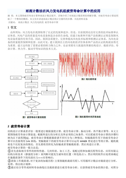
本文主要围绕疲劳寿命计算叙述,根据所进行的分析以及所必须的已知条件,可以把疲劳寿命计算的步骤归纳为以下流程图[1]。
疲劳寿命计算根据载荷谱不同可分为三种情况:恒幅载荷作用下的疲劳寿命计算可以直接利用S-N曲线;变幅载荷下的疲劳寿命计算可以运用MINER理论进行等效计算;随机载荷是个比较复杂的情况,首先要将其转化为恒幅或者变幅载荷谱,然后再进行计算。
疲劳寿命计算的一般方法是:①首先获取相关零件的材料性能、几何形状、加工工艺、装配过程和加载历程等信息,应用有限元结构分析技术(静强度分析)来判断可能发生破坏的位置(即危险点);然后利用软件后处理来确定在施载荷条件下的局部应力——应变响应;②获取工作载荷谱:对于复杂的加载历程(主要指随机载荷历程),可用循环计数法对载荷进行分析、处理,得出统计规律。
③最后结合零件或材料寿命曲线以及载荷谱进行疲劳寿命分析,以获得疲劳寿命的预计值。
对照分析得到的预计值和设计要求值确定是否修改设计。
对“雨流计数法”介绍
雨流计数法简介0、前言机械的疲劳失效是机械失效的主要失效方式,因此对机械失效的主要研究是机械疲劳失效. 目前, 机械疲劳失效的研究有两个方面: 一是根据求出的载荷谱来确定加载程序在试验室或者试验台上对机械进行疲劳试验, 得出机械(材料)在该工况下的实际寿命; 二是根据机械(材料)的特性与载荷谱并且用Miner 准则来估计机械的疲劳寿命. 无论是做疲劳试验还是估计疲劳寿命, 载荷谱的统计都是问题的关键[1]。
1、雨流计数法简介雨流计数法又可称为“塔顶法”,是由英国的Matsuiski和Endo 两位工程师提出的, 距今已有50 多年。
雨流计数法主要用于工程界, 特别在疲劳寿命计算中运用非常广泛。
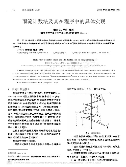
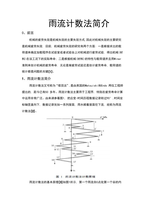
由来请参看图1, 把应变-时间历程数据记录转过90°,时间坐标轴竖直向下, 数据记录犹如一系列屋面, 雨水顺着屋面往下流, 故称为雨流计数法[2]。
雨流计数法的基本原理[3]如图1所示, 第一个雨流自0点处第一个谷的内侧流下, 从1点落1’后流至5, 然后下落。
第二个雨流从峰1点内侧流至2点落下, 由于1点的峰值低于5点的峰值,故停止。
第三个雨流自谷2点的内侧流到3, 自3点落下至3’ , 流到1’处碰上上面屋顶流下的雨流而停止。
如此下去, 可以得到如下的计数循环块:3-4-3’、1-2-1’、6-7- 6’、8-9- 8’、11-12-11、13-14-13’和12-15-12’。
雨流计数的基本流程如下。
(1) 根据采样定理作数据采集,得到时间历程记录,若截止频率为f c,则采样间隔Δt≤1/ 2f c(2) 根据连续的3个采样数据,删除既不是峰值也不是谷值的数据点,将时间历程记录转化为峰谷值序列。
(3) 针对峰谷值序列采用4点法雨流计数原则进行雨流计数,计数条件如下。
①如果A>B;B≥D;C≤A,记录一个循环 (全波) BCB′,如图 2 所示。
得到范围值S range=|B -C|幅值S a=|B -C|/ 2平均值S m=(B +C)/ 2②如果A <B;B≤D;C≥A,记录一个循环(全波) BCB′,如图 3 所示。
疲劳与断裂2.6 雨流计数法

疲劳与断裂土木工程与力学学院2.6雨流计数法工程中经常需要面对材料或结构在随机载荷作用下的寿命预测问题。
如果能够将随机载荷谱转化为变幅载荷谱,就可以利用变幅载荷谱的寿命预测方法来解决随机载荷谱的寿命预测问题。
将不规则的、随机的载荷-时间历程,转化成为一系列载荷循环的方法,称为循环计数法。
循环计数法有很多种,雨流计数法是常用的一种。
假设随机载荷谱可以看作是以典型载荷谱块为基础重复的载荷-时间历程。
通过雨流计数法,就可以识别出典型载荷谱块所包含的一系列载荷循环,从而可以将其转化为由这一系列载荷循环构成的变幅载荷-时间历程,即变幅载荷谱。
雨流计数法的主要步骤:1)从随机载荷谱中分别选取最大峰或谷处作为典型载荷谱块的起止点,如图1-1'在最大峰处起止,2-2'在最大谷处起止。
雨流计数法的主要步骤:2)将典型载荷谱块重新画在坐标图中,并顺时针旋转90º。
雨流计数法的主要步骤:2)将典型载荷谱块重新画在坐标图中,并顺时针旋转90º。
将载荷-时间历程曲线看作一个多层屋顶,假想有雨滴从最大峰或谷处开始,顺着屋面往下流。
当雨滴流至该层屋面的另一端时,若无下层屋面遮挡,雨滴反向;若有下层屋面遮挡,则雨滴落至下层屋面,并继续顺着该层屋面往下流。
雨流计数法的主要步骤:2)将典型载荷谱块重新画在坐标图中,并顺时针旋转90º。
在图中,雨滴首先从最大峰A处开始,沿屋面AB流动。
到达B点后,有下层屋面CD遮挡,因此落至屋面CD。
接下来,顺着屋面CD流至端点D,因为再无下层屋面遮挡,雨滴反向沿屋面DE流至点E。
又遇下层屋面JA'遮挡,继续下落至屋面JA'。
最后,顺着屋面JA'流至点A'。
至此,该雨滴流过的路径为ABDEA'。
雨流计数法的主要步骤:3)记录雨滴流过的路径,就可以获得一个完整的载荷循环。
载荷循环的主要参量可以从图中获得。
载荷循环ABDEA'或ADA'的应力范围,平均应力。
雨流计数法及其在程序中的具体实现
雨流计数法及其在程序中的具体实现董乐义,罗俊,程礼(西安空军工程大学工程学院,陕西西安710038) 摘 要:根据雨流计数法的规则和在实际中应用的体会,介绍了雨流计数法在程序中实现的具体方法。
它适合用各种语言编写,在计取循环数时采用的“四点法”使程序的实现比用其他方法更加准确可靠,简单明了。
关键词:计数法;程序;循环中图分类号:T P 31111;T P 30116 文献标识码:A 文章编号:100226061(2004)0320038203Ra i n Flow Coun tM ethod and Its Rea l iza tion i n Programm i ngDON G L e 2y i ,LU O J un ,CH EN G L i(A irfo rce and Engine D epartm ent of Engineering Co llege of A irfo rce Engineering U niversity,X i’an 710038,Ch ina )Abstract :A cco rd ing to the ru les of the ra in 2fl ow coun t m ethod and the exp eriences in p ractice ,th is a rticle in troduces the m ethod to rea lize the ra in 2fl ow coun t in the p rog ramm ing .It can be com p iled inva ri ou s com p u ter languages .A nd the “Fou r 2po in ts m ethod ”u sed in coun ting the l oop num ber can m akethe rea liza ti on of p rog ram m o re reliab le ,si m p le and clea r than o ther m ethod s.Key words :coun t m ethod ;p rog ram ;l oop收稿日期:2003210228作者简介:董乐义(19742),在读研究生,专业方向为航空发动机可靠性与使用寿命研究。
雨流计数法

3Rainflow Cycle CountingJ Problem Description 62J Set Up the Fatigue Analysis 63J Run the Fatigue Analysis 69J Review the Results 72J Concluding Remarks 78MSC Fatigue 2005 QuickStart Guide62Problem DescriptionProblem DescriptionThis example is an extension of the previous example where the simple constant amplitude loading isreplaced with a more complex randomly varying time signal.Invoke Pre&Post or MSC Patran by typing the following symbols at the system prompt or from a DOSwindow:fXX or fatX or fatigue where XX is the version numberp3or patranIf you have not already, open the same database that you created in the previous example working in thesame directory from the File | Open menu. The name of the database should be keyhole.Objective•To predict the life of the keyhole subject to a varying load signal.•To understand how to normalize the FE stresses.•To introduce the concept to rainflow cycle counting.•To introduce the concept of damage summation.•To investigate the effect of mean stress.•To investigate the probabilistic nature of fatigue.Note:The geometry and materials information are identical to that of the previous exercise.Chapter3: Rainflow Cycle Counting63Set Up the Fatigue Analysis Set Up the Fatigue AnalysisTo begin setup for a fatigue analysis press the Analysis switch in Pre&Post (or from the Tools pulldown menu in MSC Patran, select MSC Fatigue and then Main Interface). This will bring up the MSC Fatigue main form from which all parameters, loading and materials information, and analysis control are accessed.Load the Previous S-N Analysis ParametersMSC Fatigue 2005 QuickStart Guide Set Up the Fatigue Analysis 64Instead of defining all the analysis parameters again, let us begin from the last analysis. Once the form is open, type the jobname of the previous example in the Jobname databox (simple_sn ) and issue a carriage return (Return or Enter). You will be prompted to read in an old analysis setup file (it detects a file called simple_sn.fin in your local directory and reads in the parameters).Now change the jobname and the title:1.Jobname: rf_cycle2.Title: Simple S-N Analysis, Variable LoadingLoading InformationOpen the Loading Info... form. Then press the Time History Manager button. This will launch PTIME. The time variation of the load will be defined by a signal called SAETRN which is stored in the loading central database in the MSC Fatigue installation directory.Hint:You can do the same thing in the Job Control... form with the Action set to Read SavedJob.Chapter3: Rainflow Cycle Counting65Set Up the Fatigue Analysis Copy SAETRN from the Central DatabaseWhen PTIME comes up, select Add an entry... and then Copy from central as the method of input. A form will appear that will ask for a name. Use the List button to select SAETRN from the central database.Scale the Time History LoadFrom the PTIME main menu, select Change an entry... and then Polynomial transform. We are goingto scale up the time history to represent the actual loading applied to the component. You will be asked for the Database Entry to transform and a new target file. Use the same name (SAETRN) for both and allow overwrite. The transformation from will then appear. We simply want to scale the load up so all that is needed is to input a scale factor of 10 in the second databox. Press OK when done.Finally a form appears allowing you to change any details associated with this time history. Enter the following:MSC Fatigue 2005 QuickStart Guide66Set Up the Fatigue Analysis1.Description 1: Leave as is2.Description 2: Blank this out3.Load type: Force4.Units: Newtons5.Number of fatigue equivalent units: 16.Fatigue equivalent units: Repeats7.Life results will be reported as the number of Repeats of this entire loading sequence and not asindividual stress cycles as in the previous exercise.Plot the Time HistoryPTIME returns to its main menu where you can select Plot an entry. Accept the default file, SAETRN.Note that the maximum value is close to 10,000 Newtons. As a comparison to the previous example,which oscillated in a fully reversed fashion between positive 10kN and negative 10kN, this signal variessignificantly with a very positive mean and only occasionally reaches or nears the 10kN maximum. Wetherefore would expect this loading to be less damaging with all else the same.Select File | Exit to close the plot and press or double click the eXit switch in PTIME.67Chapter 3: Rainflow Cycle Counting Set Up the Fatigue AnalysisAssociate the FE Load to its Time VariationNow back on the Loading Info... form you must associate the time variation of the load that you just created to the static FE load case. Go to the spreadsheet as was done in the previous example. Two things need to be changed on this form.1.Time History: SAETRNSelect the middle cell to make it active. Another spreadsheet (now with two rows) appears at the bottom of the form from which you select the time history file. Click on the SAETRN row anywhere with the mouse. This will replace the cell with the new time history file name.2.Load Magnitude: 10,000The next cell becomes active and a databox appears below the spreadsheet. Change this entry to 10,000. You must press a carriage return (Return or Enter) to accept the value in the databox and fill the cell in the spreadsheet. Forgetting to do this is a common error.The time variation of the loading is now associated to the static FE results. Press the OK button to close the Loading Info... form.The load magnitude acts as a divisor to normalize the stresses to obtain a stress distribution due to a unit load as in the equation σij (t)=P(t)σij /P fea , where σij and P fea are the stress tensor and load magnitude from the FE analysis, P(t) is the externally defined time variation of the loading, and σij (t) is the resulting timeNote:In the previous example we entered unity for the Load Magnitude accepting the FE load asbeing the true representation of the load and thus the stresses. The time history, UNITLOAD, scaled the stress distribution between 1 and -1 to signify the time variation of the loading. This time the time history SAETRN is used to define the actual loading as it changes with time. The FE load magnitude is therefore simply an arbitrary number used to obtain the stressdistribution. The stresses in the FE analysis need to be normalized by this FE load magnitude of 10kN, to simulate the stress distribution due to a unit load.MSC Fatigue 2005 QuickStart Guide68Set Up the Fatigue Analysisvariation of the stress tensor (at any particular location in the component). This can be done because theanalysis is linear elastic. Using linear elastic FE analysis and associating an external time variation of theloading for fatigue analysis is called the “pseudo-static” method. “It might be said that all stress analysesare basically fatigue analyses, the differences lying in the number of cycles of applied stress.” - quotefrom Carl C. Osgood, Fatigue Design (1982).Chapter3: Rainflow Cycle Counting69Run the Fatigue Analysis Run the Fatigue AnalysisYou are ready to run the fatigue analysis. Open the Job Control... form, set the Action to Full Analysis and press the Apply button. The database will close momentarily as the results information is extracted. When the database reopens, the job will have been submitted. You can then set the Action to Monitor Job and press the Apply button from time to time to view the progress. When the messageFatigue analysis completed successfullyappears, the analysis is complete. Close down the Job Control... form when done.Rainflow Cycle CountingThis analysis takes a few minutes to run to completion. The reason it takes longer than the previous example is due to the complex nature of the time signal. The program is performing a procedure called rainflow cycle counting, referred to as “preprocessing” in MSC Fatigue. Cycle counting is a mechanismto extract and count the number of stress cycles in a signal.MSC Fatigue 2005 QuickStart Guide70Run the Fatigue AnalysisThe term Rainflow is attributed to two Japanese gentlemen, Matsuishi and Endo, who invented themethod. It is based on the concept of rain drops flowing off Japanese style pagoda roofs. Time historysignals are stood on end and rain is visualized to run off of each peak or valley. Various rules wereadopted to count cycles and reversals which is beyond the scope of this text; but suffice it to say that theend result of rainflow cycle counting is a set of constant amplitude signals and a count of the number ofcycles in each. Cycle counts can be visualized as probability density functions (PDF) or as 3-dimensionalhistogram matrices as you will see later.Damage SummationIt is important to break up a variable signal into a number of constant amplitude signals in order to assessthe life from the S-N curve. The curve itself is created by a series of constant amplitude tests. So for eachcycle in the signal you must look up the proper stress from the S-N curve. What stress to look up is thejob of rainflow cycle counting. The next challenge to tackle is the summation of the damage from eachcycle in order to report a total life due to all cycles. This is accomplished by way of the Palmgren-Minerlinear damage summation law.This states that damage can be summed by determining the ratio of the number of cycles experienced tothe number of cycles to failure for a given stress range or level and then summing all the ratios for everystress range. When this number, known as Miner’s Constant, reaches unity, failure is said to haveoccurred. The predicted life is then determined by summing the percentage of life used by each stresslevel for the entire time signal. Life is then reported back as to the number of times the given time signalcan be applied before failure.71Chapter 3: Rainflow Cycle Counting Run the Fatigue AnalysisSpeeding up the AnalysisThere are two ways that you could speed up this analysis.1.First, since we already know where the failure location will be (at the point of highest stress) because of the simplicity of this model, we could have defined a Group with only this node (Node1) and specified it in the Materials Info... form. This however, would only calculate life at this one node and would ignore the rest of the model.2.Second, on the Job Control... form you can turn on the Simplified Analysis toggle. As an exercise after you finish this problem, turn this toggle ON , change the Jobname to something else and re-run the problem. Note how much faster the analysis proceeds relative to the first time. What is happening is that for a normal analysis, the rainflow procedure is being applied to each location once its stress time variation is determined. When the Simplified Analysis toggle is turned ON, the rainflow procedure is applied to the loading time history first and the FE stresses are used to scale the rainflow histogram matrix. This speeds up the analysis significantly for a complex time signal for a single load. It does however, produce slightly less accurate results. Notice the slightvariation in predicted life when you do this.Hint:This is where user-defined fatigue equivalent units come in handy, because rarely does onewant life reported in “repeats” of the time signal, but rather in more meaningful units suchas hours, miles, years, laps, missions, etc. This is accomplished by defining these user-defined units in the PTIME, loading database manager, utility. Use the Change an entry | Edit details option.MSC Fatigue 2005 QuickStart Guide72Review the ResultsReview the ResultsOpen the Results... form on the main MSC Fatigue setup form (not to be confused with the Resultsapplication switch on the main Pre&Post or MSC Patran form). With the Action set to Read Results,press Apply. The fatigue analysis results have been read into the database. You can review the lifecontour plot as you did in the previous exercise if you wish. The contour will look similar but themagnitudes will be different.Tabular ListingOn the MSC Fatigue Results... form, change the Action to List Results and press Apply. This will startthe module PFPOST which tabularly lists the fatigue analysis results. Accepting the jobname and thedefault filtering values by pressing OK a couple of times will get you to the main menu. Press or doubleclick the Most damaged nodes switch to view a tabular listing. Note the life value of approximately105.26=184,000 repeats of the signal on Node 1. This is significantly less damaging than the previousexample considering the life is reported in repeats of the time history and not as individual cycles. To getthe number of cycles, we would have to multiply the life result by the rainflow cycle count. Press Cancelto quit the listing and press or double click eXit to leave PFPOST.Chapter3: Rainflow Cycle Counting73Review the Results Histogram MatrixLet us take a look at the results of a rainflow cycle count. From the Results... form, change the Action to Optimize and press Apply (you do not need to enter a node number) on the Results... form. This will launch the module FEFAT in its design optimization mode. When it comes up, press Worst Case to automatically select the node with the lowest life prediction. Enter a Design Life of 1E6 (a million) repeats. Press the OK button. The analyzer will re-analyze the fatigue life at Node 1 and will report the life value to you. Pressing the End button will put you into the main optimization menu.Select results Display and then plot Cycles histogram. This will display a histogram plot showing the results of the rainflow cycle count for the critical location on the model. It looks a little bit like a city skyline. Note that there are quite a few cycles that have low stress ranges and that there are fewer with high stress ranges. The height of each tower represents the number of cycles at that particular stress range and mean. Each tower is used to look up damage on the S-N curve and damage is summed over all towers.A histogram cycle plot from our first example would yield only a single tower of unit height with a meanof zero.MSC Fatigue 2005 QuickStart Guide Review the Results 74Now convert the cycle histogram plot to a damage histogram plot. This is done by either returning to the main menu and selecting results Display | plot Damage histogram or with the cycle histogram plot still displayed, select Plot_type | Damage . Now you can see the damage caused by each bin. Notice that the lower stress ranges produced zero damage. All damage came from cycles in the higher stress range, which is to be expected. Select File | Exitwhen done viewing the graphics.Hint:The accuracy of the fatigue calculation is dependent on the number of towers allowed in therainflow histogram. Typically it is broken up into what are called bins which is the matrixsize. These bins can be 32x32, 64x64, or 128x128. If you want to increase the accuracy, youcan run FEFAT interactively at the critical location and specify a larger bin size.75Chapter 3: Rainflow Cycle Counting Review the ResultsEffect of Mean StressNow let us investigate the effect of mean stress on the fatigue life predictions. First remember that the S-N curve we are using was produced for an R-ratio of minus one, or no mean stress in other words. The time history used in this example has a predominately tensile mean. The initial life prediction did not take into consideration this mean stress and therefore could perhaps be giving a somewhat non-conservative answer. From FEFAT’s design optimization menu, select Sensitivity analysis | Mean stress correction (all) then press or double click the Recalculate switch. A listing showing no correction plus two mean stress correction methods appear: Goodman and Gerber. Note that both of them give more conservative answers.How is mean stress compensated for in the S-N analysis?The simple way to explain this is that for both the Goodman and Gerber methods, knowing the ultimate tensile strength (S u ) and the actual stress amplitude (σa ) and mean (σm ), an equivalent stress range with zero mean is determined. Goodman and Gerber follow these equations:σa S e -----σm S u------+ 1 Goodman =σa S e -----σm S u ------⎝⎠⎛⎞2+1 Gerber =MSC Fatigue 2005 QuickStart Guide Review the Results 76Graphically this looks like the plot to the right where, at least for Goodman, if you draw a line connecting S u to the intersection of σa and σm and then continue it on to the stress amplitude axis, this will indicate the equivalent stress S e with zero mean. This stress is then used to look up damage on the S-N curve.Probabilistic Nature of FatigueAs a final exercise in this example, let us investigate two different materials as we did in the first problem. From the main menu of FEFAT’s design optimization mode, select Material optimization . Change the material S-N curve from MANTEN_MSN to RQC100_MSN and then press or double click theRecalculate switch again. Note that RQC100_MSN , being a much higher strength steel, gives a much higher life prediction (357,000 repeats vs. 184,000 repeats) for no mean stress corrections. This means RQC100_MSN is a better material to use (or does it?). Just looking at the S-N curve might indicate this also.Press or double click the Original parameters button to put the material back to MANTEN_MSN and then press or double click the Change parameters switch and change the Design Criterion to 99. Press or double click the Recalculate switch. Note the life of approximately 85,400 repeats. Now change the material to RQC100_MSN as done earlier and press or double click the Recalculate switch. The lifeusing the higher strength steel is now only about 30,900 repeats, less than that of the lower strength steel.Note:As a stress range of a cycle becomes larger and larger, there tends to be less and less possiblevariability in the mean of that cycle. This is indicated on the cycle histogram plot since thebase of these type of plots tends to be triangular in nature, which means that as the stress gets larger, the mean stress has less of an effect on the fatigue life.Chapter3: Rainflow Cycle Counting77Review the ResultsThis is due to the probabilistic nature of fatigue and the scatter associated with the S-N curves themselves. By specifying 99 as the design criterion, we are asking MSC Fatigue to calculate a life value based on a 99% certainty of survival. The larger the scatter in the original S-N data that makes up the curve, the less certain we will be of survival and the code takes this into account by reporting a more conservative answer. The default is a 50% probability of survival (or failure)Note:Scatter is associated with S-N curves and other damage curves due to the fact that, for example, if you take 10 identical test coupons and subject them to what you think are identicaltests, you will get ten slightly different answers. The material parameters associated with S-Ncurves take this into consideration with the Standard Error of Log(N) (SE) determined byregression analysis of the raw data.MSC Fatigue 2005 QuickStart Guide78Concluding RemarksConcluding RemarksThis exercise introduced you to rainflow cycle counting, damage summation, mean stress effects, andthe probabilistic nature of fatigue by using a randomly varying load on our simple keyhole model.Though this example still did not help us identify critical locations since we already knew where failurewould occur, it did start to show the power of MSC Fatigue by being able to handle complex time signalsand to make compensation for parameters that may effect the fatigue life, something that would be adaunting task to do by hand.The next exercise will introduce the concept of a component S-N curve.Quit from Pre&Post or MSC Patran when you are through with this exerciseNote:MSC Fatigue does not take into account the frequency (speed at which cycles are experienced) or the sequence (when a particular cycle is experienced relative to other cycles) of cycles froma given signal. Rainflow cycle counting simply counts the number of cycles and determinestheir range and mean. Frequency and sequence can have an influence on the fatigue life but isa third or fourth order effect on life prediction in most cases. MSC Fatigue does provide youwith certain fatigue analysis utilities to determine if these influences are important after theinitial analysis using the MSC MSC Fatigue module MTCD (for time correlated damage).。
对“雨流计数法”介绍
雨流计数法简介0、前言机械的疲劳失效是机械失效的主要失效方式,因此对机械失效的主要研究是机械疲劳失效. 目前, 机械疲劳失效的研究有两个方面: 一是根据求出的载荷谱来确定加载程序在试验室或者试验台上对机械进行疲劳试验, 得出机械(材料)在该工况下的实际寿命; 二是根据机械(材料)的特性与载荷谱并且用Miner 准则来估计机械的疲劳寿命. 无论是做疲劳试验还是估计疲劳寿命, 载荷谱的统计都是问题的关键[1]。
1、雨流计数法简介雨流计数法又可称为“塔顶法”,是由英国的Matsuiski和Endo 两位工程师提出的, 距今已有50 多年。
雨流计数法主要用于工程界, 特别在疲劳寿命计算中运用非常广泛。
由来请参看图1, 把应变-时间历程数据记录转过90°,时间坐标轴竖直向下, 数据记录犹如一系列屋面, 雨水顺着屋面往下流, 故称为雨流计数法[2]。
雨流计数法的基本原理[3]如图1所示, 第一个雨流自0点处第一个谷的内侧流下, 从1点落1’后流至5, 然后下落。
第二个雨流从峰1点内侧流至2点落下, 由于1点的峰值低于5点的峰值,故停止。
第三个雨流自谷2点的内侧流到3, 自3点落下至3’ , 流到1’处碰上上面屋顶流下的雨流而停止。
如此下去, 可以得到如下的计数循环块:3-4-3’、1-2-1’、6-7- 6’、8-9- 8’、11-12-11、13-14-13’和12-15-12’。
雨流计数的基本流程如下。
(1) 根据采样定理作数据采集,得到时间历程记录,若截止频率为f c,则采样间隔Δt≤1/ 2f c(2) 根据连续的3个采样数据,删除既不是峰值也不是谷值的数据点,将时间历程记录转化为峰谷值序列。
(3) 针对峰谷值序列采用4点法雨流计数原则进行雨流计数,计数条件如下。
①如果A>B;B≥D;C≤A,记录一个循环 (全波) BCB′,如图 2 所示。
得到范围值S range=|B -C|幅值S a=|B -C|/ 2平均值S m=(B +C)/ 2②如果A <B;B≤D;C≥A,记录一个循环(全波) BCB′,如图 3 所示。
雨流计数法的应用
• 首先应明确有限元模型对几何模型进行了 离散化。这就使几何模型与有限元模型产 生了差异。
精品课件
• 过盈配合所致的接触分析的难点在于如何 确定初始接触状态。初始接触状态设置得 不对,会导致错误的计算结果或者不准确 的计算结果
精品课件
• 因此若想通过几何来模拟过盈配合,应该 尽量细化接触面的网格,但同时也增加了 计算量。
• 峰谷值提取:顺序读入数据,计算i点数据 与i-1点、i+1点和i点数据的差值相乘。若 积小于0,则存储i点数据,否则读入下一 点。
• 无效幅值去除:给定判断条件(如指定数 据最大差程的10%),顺序读入数据,计算 计算i点数据与i-1点、i+1点和i点数据的 差的绝对值,如果均大于等于判定条件, 则存储i点数据,否则读入下一点。
得到更平滑、精确 的响应曲线 允许考虑模态阻尼
比完全法快
计算费用高
恒定时间步长 不能计算非线性, 只能包含简单的点 点接触 不能施加强制非零 位移
精品课件
需要扩展得到完整 结果 不能施加单元载荷
所有载荷必须施加 在主自由度上 时间步长恒定
只支持简单的点点 接触
完全法求解瞬态动力学的问题
• 阻尼比如何确定 • 时间步长的确定,关心的响应频率如何确
定?是否只关心比激振力频率小的固有频 率就可以了? • 是否要分别对整体模型和单隔板模型分别 进行模态分析来修正单隔板模型的边界条 件。(部分模态会丢失,影响结构的响应)
精品课件
问题和工作
• 问题 • 应用何种方法(完全法、模态叠加法) • 时间步长的确定,哪些是关心频率
(Δt=1/20f) • 模型(装配体、整体分析) • 工作 • 简化模型去掉或等效接触 • 减少单元数量 • 设置合适的时间步长
雨流计数法
疲劳分析中的雨流计数法这种方法的突出特点是根据所研究材料的应力-应变之间的非线性关系来进行计数,亦即把样本记录用雨流法定出一系列闭合的应力-应变滞后环。
参看图1,把应变-时间历程样本记录转过90°,时间坐标轴竖直向下,样本记录犹如一系列屋面,雨水顺着屋面往下流,故称为雨流法。
雨流法有下列规则:(ⅰ)雨流在试验记录的起点和依此在每一个峰值的内边开始,亦即从1,2,3…等尖点开始。
(ⅱ)雨流在流到峰值处(即屋檐)竖直下滴,一直流到对面有一个比开始时最大值(或最小值)更正的最大值(或更负的最小值)为止。
(ⅲ)当雨流遇到来自上面屋顶流下的雨时,就停止流动。
(ⅳ)如果初始应变为拉应变,顺序的始点是拉应变最小值的点。
(ⅴ)每一雨流的水平长度是作为该应变幅值的半循环计数的.在图1中,雨流法从1点开始,该点认为是最小值。
雨流流至2点,竖直下滴到3与4点幅值间的2ˊ点,然后流到4点,最后停于比1点更负的峰值5的对应处。
得出一个从1到4的半循环。
下一个雨流从峰值2点开始,流经3点,停于4点的对面,因为4点是比开始的2点具有更正的最大值,得出一个半循环2-3。
第三个流动从3点开始,因为遇到由2点滴下的雨流,所以终止于2ˊ点,得出半循环3-2ˊ。
这样,3-2和2-3就形成了一个闭合的应力-应变回路环,它们配成一个完全的循环2′-3-2。
下一个雨流从峰值4开始,流经5点,竖直下滴到6和7之间的5ˊ点,继续往下流,再从7点竖直下滴到峰值10的对面,因为10点比4点具有更正的最大值。
得出半循环4-5-7。
第五个流动从5点开始,流到6点,竖直下滴,终止于7点的对面,因为7点比5点具有更负的极小值。
取出半循环5-6。
第六个流动从6点开始,因为遇到由5点滴下的雨滴,所以流到5ˊ点终止。
半循环6-5与5-6配成一个完全循环5ˊ-6-5,取出5ˊ-6-5。
第七个流动从7点开始,经过8点,下落到9-10线上的8ˊ点,然后到最后的峰值10,取出半循环7-8-10。
python rainflow原理
Rainflow分析是用于疲劳寿命预测的一种方法,主要用于分析循环加载历程中的应力或应变信号。
这个方法通过识别并计数信号中的载荷循环,从而允许工程师估计材料或结构在疲劳加载下的寿命。
Rainflow分析的原理如下:
1.载荷历程分段:Rainflow分析首先将载荷历程分段为不同的循环。
这些循环可以是正循环(正载荷到零载荷到负载荷再到零载荷的过程)或负循环。
分段通常使用计数法或零穿越法。
2.循环计数:对于每个循环,Rainflow分析会计数它的幅值和平均值。
这些值称为振幅和偏移。
振幅是循环的最大值和最小值之间的差,偏移是这个差的一半。
3.Rainflow循环计数矩阵:创建一个Rainflow循环计数矩阵,其中行表示振幅范围的范围,列表示平均值的范围。
在这个矩阵中,每个元素表示在相应的振幅和平均值范围内发生的循环的次数。
4.等效循环计算:根据Rainflow循环计数矩阵,可以计算等效循环。
等效循环是一种简化的度量,将不同振幅和平均值的循环统一为一个具有相同疲劳寿命影响的循环。
5.寿命估计:利用等效循环和材料的疲劳曲线,可以估计材料或结构在给定载荷历程下的疲劳寿命。
Rainflow分析的优势在于它能够处理复杂的载荷历程,并提供了一种在不同载荷水平和循环次数下进行疲劳寿命评估的方法。
这种方法常用于材料疲劳寿命预测、结构健康监测和工程设计等领域。
雨流计数法及其在疲劳寿命估算中的应用
5.875 2675 891 400 194 69
25
4
2
在恒定应力水平下,疲劳寿命分布一般 115.375 1016 91
1
0
0
0
0
0
服从对数正态分布,并且由恒定应力下的寿 224.875 131 8
0
0
0
0
0
0
命样本,可以计算寿命分布均值和方差[ 7 ]。 334.375 15
0
0
0
0
0
0
0
443.875 2
载荷谱[ 3 ]。如果
载荷均值
这个载荷谱是在 工作频次 1 2 … j … n
用户使用条件下
测量得到的,那
么它就是用户使 载 用条件下的载荷 荷
1 2 ∶
Sm1 Sa1
Sa2 ∶
Sm2
…
Smj
Smn
谱,如果是在试 幅 车场条件下得到 值
i Sai ∶∶
nij
的,它就是该构 件在试车场条件
(3) 生成不同均幅值载荷下的疲劳寿命表 Nij 把
得到的 Sij 代入式 (3) 中,并根据给定的 P 值查得的
up,从而得到均幅值载荷表中的
N
。如
ij
p
= 0.5,up=
0,由S1 = 92.15 MPa,可得
0 = lg N + 0.003 331× 92.15-6.921 155 0 .196 401 − 0 .000 198 × 92 .15
0
0
0
0
0
0
0
∫ p = 1 − N Nmin
f (N/
S)dN (1)
式中 f(N/ S) 为在应力水平 S 下疲劳寿