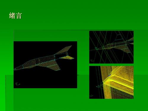
详细FLUENT实例讲座翼型计算
Fluent关于飞机的非常详细的算例
无量纲化
参数:参考面积s=26.15m2 特征长度 cl=8.32m b=3.79m 动压q=0.5*ρ *v2 F升 M滚 C升 C滚 qs q s cl
F阻 C阻 qs F侧 C侧 qs
C俯 C偏
M俯 q s cl M偏 qsb
工况a: 1.535马赫
尾翼和机体交线过于复杂尾翼和机体交线过于复杂解决办法解决办法机翼与机体分离机翼与机体分离解决办法解决办法围机翼时候围机翼时候uuvv失败解决办法失败解决办法飞机的几何翻转注意点并线时候遇到问题飞机的几何翻转注意点并线时候遇到问题及解决办法及解决办法计算区域计算区域虚面的出现及影响虚面的出现及影响先将所有体围好后做网格的坏处先将所有体围好后做网格的坏处有的体很难划分结构化网格需要对几何有的体很难划分结构化网格需要对几何体进行改动体进行改动一个体的改动会牵动相邻的体进而波及一个体的改动会牵动相邻的体进而波及更多的体更多的体导致返工导致返工网格先从机翼处开始做的好处网格先从机翼处开始做的好处机翼根部网格最为复杂机翼根部网格最为复杂从两头往里做的话一旦到这儿遇到问题从两头往里做的话一旦到这儿遇到问题难以避开的话势必要返工前面的网格
来流速度1.535马赫 飞机仰角4度
工况a
工况a
升力系数 试验结果 (未修正) 计算结果 (Euler) 0.2179
阻力系数 0.0390
0.217
变换仰角的计算结果
仰角(单 0 位:度) 升力 系数 阻力 系数 2 4 6 8
0.0305 0.1250 0.2173 0.3138 0.4101
绪言
网格的工具,机器配置
gambit, 双奔3◎866mhz,2G内存
数据处理
原始数据文件给出了点座标。 数据的整理和读入,journel文件
FLUENT翼型算例 - Flow over an Airfoil- Problem Specification教程
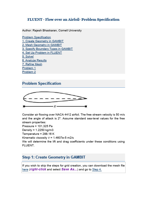
FLUENT - Flow over an Airfoil- Problem SpecificationConsider air flowing over NACA 4412 airfoil. The free stream velocity is 50 m/s and the angle of attack is 2°. Assume standard sea-level values for the free stream properties:Pressure = 101,325 PaDensity = 1.2250 kg/m3Temperature = 288.16 KKinematic viscosity v = 1.4607e-5 m2/sWe will determine the lift and drag coefficients under these conditions using FLUENT.Higher Resolution ImageThis tutorial leads you through the steps for generating a mesh in GAMBIT for an airfoil geometry. This mesh can then be read into FLUENT for fluid flow simulation.In an external flow such as that over an airfoil, we have to define a far field boundary and mesh the region between the airfoil geometry and the far field boundary. It is a good idea to place the far field boundary well away from the airfoil since we'll use the ambient conditions to define the boundary conditions at the far field. The farther we are from the airfoil, the less effect it has on the flow and so more accurate is the far field boundary condition.The far field boundary we'll use is the line ABCDEFA in the figure above. c is the chord length.Start GAMBITCreate a new directory called airfoil and start GAMBIT from that directory by typing gambit -id airfoil at the command prompt.Under Main Menu, select Solver > FLUENT 5/6 since the mesh to be created is to be used in FLUENT 6.0.Import EdgeTo specify the airfoil geometry, we'll import a file containing a list of vertices along the surface and have GAMBIT join these vertices to create two edges, corresponding to the upper and lower surfaces of the airfoil. We'll then split these edges into 4 distinct edges to help us control the mesh size at the surface.The file containing the vertices for the airfoil can be downloaded here: naca4412.dat (right click and select Save As...)Let's take a look at the naca4412.dat file:255 20 0 0-0.00019628 0.001241474 0-0.000247836 0.001759397 0-0.000275577 0.002158277 0-0.000290986 0.002495536 0-0.000298515 0.002793415 0-0.000300443 0.00306332 0The first line of the file represents the number of points on each edge (255) and the number of edges (2). The first 255 set of vertices are connected to form the edge corresponding to the upper surface; the next 255 are connected to form the edge for the lower surface.The chord length, c for the geometry in naca4412.dat file is 1, so x varies between 0 and 1. If you are using a different airfoil geometry specification file, note the range of x values in the file and determine the chord length c. You will need this later on.Main Menu > File > Import > ICEM Input ...For File Name, browse and select the naca4412.dat file. Select both Vertices and Edges under Geometry to Create: since these are the geometric entities we need to create. Deselect Face. Click Accept.Higher Resolution ImageWe have more points around the nose area because of the high curvature around the nose.Create Far field BoundaryNext, we will create the following far field boundary. This picture of thefarfield nomenclaturewill be handy.We will create the far field boundary by creating vertices and joining them appropriately to form edges.Operation Tool pad > Geometry Command Button> Vertex Command Button> Create VertexCreate the following vertices by entering the coordinates under Global and the label under Label:Click the FIT TO WINDOW button to scale the display so that you can see all the vertices. The resulting image should look like this:Higher Resolution ImageNow we can create the edges using the vertices created.Operation Tool pad > Geometry Command Button> Edge Command Button> Create EdgeCreate the edge AB by selecting the vertex A followed by vertex B. Enter AB for Label. Click Apply. GAMBIT will create the edge. You will see a message saying something like "Created edge: AB'' in the Transcript window. Similarly, create the edges BC, CD, DE, EG, GA and CG. Note that you might have to zoom in on the airfoil to select vertex G correctly or click on the to select the vertices from the list and move them to the picked list. The rest of the tutorial will use this method for vertices selection.Next we'll create the circular arc AF. Right-click on the Create Edge button and select Arc.In the Create Real Circular Arc menu, the box next to Center will be yellow. That means that the vertex you select will be taken as the center of the arc. Select vertex G and click Apply. Now the box next to End Points will be highlighted in yellow. This means that you can now select the two vertices that form the end points of the arc. Select vertex A and then vertex F. Enter AF under Label. Click Apply.If you did this right, the arc AF will be created. If you look in the transcript window, you'll see a message saying that an edge has been created. Similarly, create an edge corresponding to arc EF.Higher Resolution ImageCreate FacesThe edges we have created can be joined together to form faces. We will need to define three faces as shown in the image above. Two rectangular faces, rect1 and rect2 lie to the right of the airfoil. The third face, circ1 consists of the area outside of the airfoil but inside of the semi-circular boundary.Operation Tool pad > Geometry Command Button> Face Command Button> Form FaceThis brings up the Create Face From Wireframe menu. Recall that we had selected vertices in order to create edges. Similarly, we will select edges in order to form a face.To create the face rect1, select the edges AB, BC, CG, and GA. Enter rect1for the label and click Apply. GAMBIT will tell you that it has "Created face: rect1'' in the transcript window.Similarly, create the face rect2 by selecting ED, DC, CG and GE.To create the last face we will need to make two separate faces, one for the outer boundary and one for the airfoil and then subtract the airfoil from the boundary. Create semi-circular face circ1 by selecting GA, AF, FE and EG and enter circ1 for the label. Create the face for the airfoil by selecting corresponding edges. Subtract the airfoil from circ1.Operation Tool pad > Geometry Command Button> Face Command Buttonright click on the Boolean Operations Button and select SubtractThe Face box will be highlighted yellow. Shift click to select circ1, the outer semi-circular boundary. Then select the lower box labeled Subtract Faces which will allow you to select faces to subtract from our outer boundary. Select the airfoil face and click apply.Mesh FacesWe'll mesh each of the 3 faces separately to get our final mesh. Before we mesh a face, we need to define the point distribution for each of the edges that form the face i.e. we first have to mesh the edges. We'll select the mesh stretching parameters and number of divisions for each edge based on three criteria:1. We'd like to cluster points near the airfoil since this is where the flow is modified the most;the mesh resolution as we approach the far field boundaries can become progressively coarser since the flow gradients approach zero.2. Close to the surface, we need the most resolution near the leading and trailing edgessince these are critical areas with the steepest gradients.3. We want transitions in mesh size to be smooth; large, discontinuous changes in the meshsize significantly decrease the numerical accuracy.The edge mesh parameters we'll use for controlling the stretching are successive ratio, first length and last length. Each edge has a direction as indicated by the arrow in the graphics window. The successive ratio R is the ratio of the length of any two successive divisions in the arrow direction as shown below. Go to the index of the GAMBIT User Guide and look under Edge>Meshing for this figure and accompanying explanation. This help page also explains what the first and last lengths are; make sure you understand what they are.Operation Tool pad > Mesh Command Button> Edge Command Button> Mesh EdgesSelect the edge GA. The edge will change color and an arrow and several circles will appear on the edge. This indicates that you are ready to mesh this edge. Make sure the arrow is pointing upwards. You can reverse the direction of the edge by clicking on the Reverse button in the Mesh Edges menu.Enter a ratio of 1.15. This means that each successive mesh division will be1.15 times bigger in the direction of the arrow. Select Interval Count underSpacing. Enter 45 for Interval Count. Click Apply. GAMBIT will create 45 intervals on this edge with a successive ratio of 1.15.For edges AB and CG, we'll set the First Length (i.e. the length of the division at the start of the edge) rather than the Successive Ratio. Repeat the same steps for edges BC, AB and CG with the following specifications:Note that later we'll select the length at the trailing edge to be 0.02c so that the mesh length is continuous between IG and CG, and HG and CG.Now that the appropriate edge meshes have been specified, mesh the face rect1:Operation Tool pad > Mesh Command Button> Face Command Button> Mesh FacesSelect the face rect1. The face will change color. You can use the defaults of Quad (i.e. quadrilaterals) and Map. Click Apply.The meshed face should look as follows:Higher Resolution ImageNext mesh face rect2 in a similar fashion. The following table shows the parameters to use for the different edges:The resultant mesh should be symmetric about CG as shown in the figure below.Higher Resolution ImageSplit EdgesNext, we will split the top and bottom edges of the airfoil into two edges so that we have better control of the mesh point distribution. Figure of the splitting edges is shown below.We need to do this because a non-uniform grid spacing will be used for x<0.3c and a uniform grid spacing for x>0.3c. To split the top edge into HI and IG, selectOperation Tool pad > Geometry Command Button> Edge Command Button> Split/Merge EdgeMake sure Point is selected next to Split With in the Split Edge window. Select the top edge of the airfoil by Shift-clicking on it.We'll use the point at x=0.3c on the upper surface to split this edge into HI and IG. To do this, enter 0.3 for x: under Global. If your c is not equal to one, enter the value of 0.3*c instead of just 0.3.For instance, if c=4, enter 1.2. From here on, whenever you're asked to enter (some factor)*c, calculate the appropriate value for your c and enter it.Click Apply. You will see a message saying "Edge edge.1 was split, and edge edge.3 created'' in the Transcript window.Repeat this procedure for the lower surface to split it into HJ and JG. Use the point at x=0.3c on the lower surface to split this edge.Higher Resolution ImageFinally, let's mesh the face consisting of circ1 and the airfoil surface. For edges HI and HJ on the front part of the airfoil surface, use the following parameters to create edge meshes:For edges IG and JG, we'll set the divisions to be uniform and equal to 0.02c. Use Interval Size rather than Interval Count and create the edge meshes:For edge AF, the number of divisions needs to be equal to the number of divisions on the line opposite to it, in this case, the upper surface of the airfoil(this is a subtle point; chew over it). To determine the number of divisions that GAMBIT has created on edge IG, selectOperation Tool pad > Mesh Command Button> Edge Command Button>Summarize Edge MeshSelect edge IG and then Elements under Component and click Apply. This will give the total number of nodes (i.e. points) and elements (i.e. divisions) on the edge in the Transcript window. The number of divisions on edge IG is35. (If you are using a different geometry, this number will be different; I'll refer to it as NIG). So the Interval Count for edge AF is NHI+NIG= 40+35= 75. Similarly, determine the number of divisions on edge JG. This comes out as 35 for the current geometry. So the Interval Count for edge EF is 75.Create the mesh for edges AF and EF with the following parameters:Mesh the face. The resultant mesh is shown below.Higher Resolution ImageWe'll label the boundary AFE as farfield1, ABDE as farfield2 and the airfoil surface as airfoil. Recall that these will be the names that show up under boundary zones when the mesh is read into FLUENT.Group EdgesWe'll create groups of edges and then create boundary entities from these groups.First, we will group AF and EF together.Operation Tool pad > Geometry Command Button > Group Command Button > Create GroupSelect Edges and enter farfield1 for Label, which is the name of the group. Select the edges AF and EF.Note that GAMBIT adds the edge to the list as it is selected in the GUI.Click Apply.In the transcript window, you will see the message "Created group: farfield1 group".Similarly, create the other two far field groups. You should have created a total of three groups:Define Boundary TypesNow that we have grouped each of the edges into the desired groups, we can assign appropriate boundary types to these groups.Operation Tool pad > Zones Command Button> Specify Boundary TypesUnder Entity, select Groups.Select any edge belonging to the airfoil surface and that will select the airfoil group. Next to Name:, enter airfoil. Leave the Type as WALL.Click Apply.In the Transcript Window, you will see a message saying "Created Boundary entity: airfoil".Similarly, create boundary entities corresponding to farfield1, farfield2 and farfield3groups. Set Type to Velocity-Inlet for farfield1and farfield2. Set Type to Pressure-Outlet for farfield3.Save Your WorkMain Menu > File > SaveExport MeshMain Menu > File > Export > Mesh...Save the file as airfoil.msh.Make sure that the Export 2d Mesh option is selected.Check to make sure that the file is created.Launch FLUENTStart > Programs > Fluent Inc > FLUENT 6.3.26Select 2ddp from the list of options and click Run.Import FileMain Menu > File > Read > Case...Navigate to your working directory and select the airfoil.msh file. Click OK. The following should appear in the FLUENT window:Check that the displayed information is consistent with our expectations of the airfoil grid.Analyze GridGrid > Info > SizeHow many cells and nodes does the grid have?Display > GridNote what the surfaces farfield1, farfield2, etc. correspond to by selecting and plotting them in turn.Zoom into the airfoil.Where are the nodes clustered? Why?Define PropertiesDefine > Models > Solver...Under the Solver box, select Pressure Based.Click OK.Define > Models > ViscousSelect Inviscid under Model.Click OK.Define > Models > EnergyThe speed of sound under SSL conditions is 340 m/s so that our free stream Mach number is around 0.15. This is low enough that we'll assume that the flow is incompressible. So the energy equation can be turned off.Make sure there is no check in the box next to Energy Equation and click OK.Define > MaterialsMake sure air is selected under Fluid Materials. Set Density to constant and equal to 1.225 kg/m3.Click Change/Create.Define > Operating ConditionsWe'll work in terms of gauge pressures in this example. So set Operating Pressure to the ambient value of 101,325 Pa.Click OK.Define > Boundary ConditionsSet farfield1 and farfield2 to the velocity-inlet boundary type.For each, click Set.... Then, choose Components under Velocity Specification Method and set the x- and y-components to that for the free stream. For instance, the x-component is 50*cos(1.2)=49.99. (Note that 1.2° is used as our angle of attack instead of 2°to adjust for the error caused by assuming the airfoil to be 2D instead of 3D.)Click OK.Set farfield3to pressure-outlet boundary type, click Set...and set the Gauge Pressure at this boundary to 0. Click OK.Solve > Control > SolutionTake a look at the options available.Under Discretization, set Pressure to PRESTO!and Momentum to Second-Order Upwind.(click picture for larger image)Click OK.Solve > Initialize > Initialize...As you may recall from the previous tutorials, this is where we set the initial guess values (the base case) for the iterative solution. Once again, we'll set these values to be equal to those at the inlet (to review why we did this look back to the tutorial about CFG programs). Select farfield1 under Compute From.Click Init.Solve > Monitors > Residual...Now we will set the residual values (the criteria for a good enough solution). Once again, we'll set this value to 1e-06.(click picture for larger image)Click OK.Solve > Monitors > Force...Under Coefficient, choose Lift. Under Options, select Print and Plot. Then, Choose airfoil under Wall Zones.Lastly, set the Force Vector components for the lift. The lift is the force perpendicular to the direction of the free stream. So to get the lift coefficient, set X to -sin(1.2°)=-020942 and Y to cos(1.2°)=0.9998.(click picture for larger image)Click Apply for these changes to take effect.Similarly, set the Force Monitor options for the Drag force. The drag is defined as the force component in the direction of the free stream. So under Force Vector, set X to cos(1.2°)=0.9998 and Y to sin(1.2°)=0.020942 Turn on only Print for it.Report > Reference ValuesNow, set the reference values to set the base cases for our iteration. Select farfield1 under Compute From.Click OK.Note that the reference pressure is zero, indicating that we are measuring gage pressure.Main Menu > File > Write > Case...Save the case file before you start the iterations.Solve > IterateMake note of your findings, make sure you include data such as;What does the convergence plot look like?How many iterations does it take to converge?How does the Lift coefficient compared with the experimental data?Main Menu > File > Write > Case & Data...Save case and data after you have obtained a converged solution.Lift CoefficientThe solution converged after about 480 iterations.476 1.0131e-06 4.3049e-09 1.5504e-09 6.4674e-01 2.4911e-03 0:00:48 524! 477 solution is converged477 9.9334e-07 4.2226e-09 1.5039e-09 6.4674e-01 2.4910e-03 0:00:38 523From FLUENT main window, we see that the lift coefficient is 0.647. This compare fairly well with the literature result of 0.6 from Abbott et al.Plot Velocity VectorsLet's see the velocity vectors along the airfoil.Display > VectorsEnter 4 next to Scale. Enter 3 next to Skip. Click Display.Higher Resolution ImageAs can be seen, the velocity of the upper surface is faster than the velocity on the lower surface.White Background on Graphics WindowTo get white background go to:Main Menu > File > HardcopyMakeselectprompted "Higher Resolution ImageOn the leading edge, we see a stagnation point where the velocity of the flow is nearly zero. The fluid accelerates on the upper surface as can be seen from the change in colors of the vectors.Higher Resolution ImageOn the trailing edge, the flow on the upper surface decelerates and converge with the flow on the lower surface.Do note that the time for fluid to travel top and bottom surface of the airfoil is not necessarily the same, as common misconceptionPlot Pressure CoefficientPressure Coefficient is a dimensionless parameter defined by the equationwhere p is the static pressure,P ref is the reference pressure, andq ref is the reference dynamic pressure defined byThe reference pressure, density, and velocity are defined in the Reference Values panel in Step 5. Please refer to FLUENT's help for more information. Go to Help > User's Guide Index for help.Plot > XY Plot...Change the Y Axis Function to Pressure..., followed by Pressure Coefficient. Then, select airfoil under Surfaces.Click Plot.Higher Resolution ImageThe lower curve is the upper surface of the airfoil and have a negative pressure coefficient as the pressure is lower than the reference pressure.Plot Pressure ContoursPlot static pressure contours.Display > Contours...Select Pressure... and Pressure Coefficient from under Contours Of. Check the Filled and Draw Grid under Options menu. Set Levels to 50.Click Display.Higher Resolution ImageFrom the contour of pressure coefficient, we see that there is a region of high pressure at the leading edge (stagnation point) and region of low pressure on the upper surface of airfoil. This is of what we expected from analysis of velocity vector plot. From Bernoulli equation, we know that whenever there is high velocity, we have low pressure and vise versa.Force ConventionsFLUENT report forces in term of pressure force and viscous force. For instance, we are interested in the drag on the airfoil,(Drag)total = (Drag)pressure + (Drag)viscousDrag due to pressure:Drag due to viscous effect:wheree d is the unit vector parallel to the flow direction.n is unit vector perpendicular to the surface of airfoil.t is unit vector parallel to the surface of airfoil.Similarly, if we are interested in the lift on the airfoil,(Lift) = (Lift)pressure + (Lift)viscousLift due to pressure:Lift due to viscous effect:Report ForceWe will first investigate the Drag on the airfoil.Main Menu > Report > Forces...Select Forces. Under Force Vector, enter 0.9998 next to X. Enter 0.02094 next to Y. Select airfoil under Wall Zones. Click Print.Here's is what we see in the main menu:C d = (C d)pressure + (C d)skin frictionwhere(C d)pressure is due to pressure force.(C d)skin friction is due to viscous force.Indeed, we see that the (C d)skin friction is zero because of the inviscid model.In reality, (Cof the inviscid model that we specify. (Czerocomputation.Now, let's look at the lift coefficient.Main Menu > Report > Forces...Select Forces. Under Force Vector, enter -0.02094 next to X. Enter 0.9998 next to Y. Select airfoil under Wall Zones. Click Print.Here's is what we see in the main menu:Similarly, lift force is due to the contribution of pressure force and viscous force.C l = (C l)pressure + (C l)skin frictionwhere(C l)pressure is due to pressure force.(C l)skin friction is due to viscous force.Since our model is inviscid, (C l)skin friction is zero. We see that the lift coefficient compare well with the experimental value of 0.6.Doexperimental value. In reality, if we take into account the effect of viscosity,Grid ConvergenceA finer mesh with four times the original mesh density was created. The lift coefficient was found to be 0.649.We see that the difference in drag coefficient is very large. We used inviscid case for our model, so we are expecting a C d of zero. However, since the parameter of interest is the lift coefficient, and the value lift coefficient does not deviate much from original mesh to fine mesh, we concluded that the fine mesh is good enough.Thevalidation steps are needed before we can conclude about the accuracy of our model. Other parameter that will affect the validity of our result is the choice of viscous model. We used inviscid model which basically assumed that the flow inviscid and totally ignore the effect of boundary layer near the airfoilReynolds number flow.SummaryFollowing table shows comparison of modeling result with experimental data.Though further validation steps are still needed before we can come up with a model that will accurately represent the physical flow, this simple tutorial demonstrates the use of reasonable assumption and approximation in obtaining understanding of physical flow properties around an airfoil. ReferenceThe experimental data is taken from Theory of Wing Sections By Ira Herbert Abbott, Albert Edward Von Doenhoff pg. 488Google scholar linkConsider the incompressible, inviscid airfoil calculation in FLUENT presented in class. Recall that the angle of attack, α, was 5°.Repeat the calculation for the airfoil for α = 0° and α = 10°. Save your calculation for each angle of attack as a different case file.(a) Graph the pressure coefficient (C p) distribution along the airfoil surface at α = 5° and α = 10° in the manner discu ssed in class (i.e., follow the aeronautical convention of letting C p decrease with increasing ordinate (y-axis) values).What change do you see in the C p distribution on the upper and lower surfaces as you increase the angle of attack?Which part of the airfoil surface contributes most to the increase in lift with increasing α?Hint: The area under the C p vs. x curve is approximately equal to C l.(b) Make a table of C l and C d values obtained for α = 0°, 5°, and 10°. Plot C l vs.α for the three values of α. Make a linear least squares fit of this data and obtain the slope. Compare your result to that obtained from inviscid, thinairfoil theory:,where α is in degrees.Repeat the incompressible calculation at α = 5° including viscous effects. Since the Reynolds number is high, we expect the flow to be turbulent. Use the k-ε turbulence model with the enhanced wall treatment option. At the far field boundaries, set turbulence intensity=1% and turbulent length scale=0.01.(a) Graph the pressure coefficient (C p) distribution along the airfoil surface for this calculation and the inviscid calculation done in the previous problem at α = 5°. Comment on any differences you observe.(b) Compare the C l and C d values obtained with the corresponding values from the inviscid calculation. Discuss briefly the similarities and differences between the two results.。
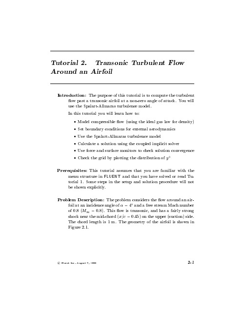
fluent计算跨音速翼型教程
c Fluent Inc. August 7, 1998
2-1
Transonic Turbulent Flow Around an Airfoil
α = 4° M∞= 0.8
1m
Figure 2.1: Problem Speci cation
Preparation
1. Copy the le
fluent_inc fluent5 tut airfoil airfoil.msh
Extra: You can use the right mouse button to check which
zone number corresponds to each boundary. If you click the right mouse button on one of the boundaries in the graphics window, its zone number, name, and type will be printed in the FLUENT console window. This feature is especially useful when you have several zones of the same type and you want to distinguish between them quickly.
3. Turn on the Spalart-Allmaras turbulence model.
De ne ,! Models ,!Viscous...
a Select the Spalart-Allmaras model and retain the default options and constants.
fluent处理三维机翼数据及用相关软件绘制三维翼型过程
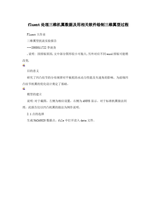
fluent处理三维机翼数据及用相关软件绘制三维翼型过程Fluent大作业三维翼型扰流实验报告---2008011722李凌尧,说明: 因排版原因,文中部分图形较小可拖大,另外对应不同word排版可能稍改变,目的意义研究了凹凸结节的分布规律对平板舵的水动力性能及失速角的影响,为前缘凹凸结节机翼的优化设计奠定了基础。
模型的建立说明:对于截图,左侧为相应设置,右侧为ANSYS显示。
对于标准机翼做法同理,此报告仅以凹凸机翼的做法为例作说明。
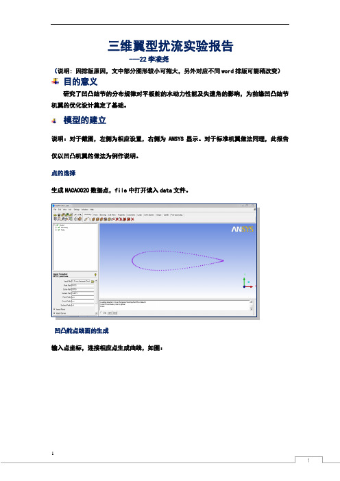
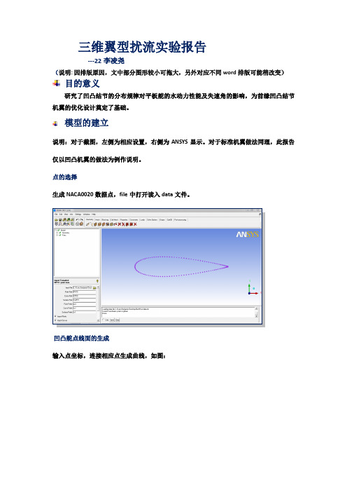
2.1点的选择生成NACA0020数据点,file中打开读入data文件。
凹凸舵点线面的生成 2.2输入点坐标,连接相应点生成曲线,如图: 1Fluent大作业再根据曲线建立面2.3生成流域输入点坐标、连接相应点生成曲线,由相应曲线建立面,然后再生成体如图: 2Fluent大作业2.4生成新的part关闭点和线以及体,只留面。
选择part---create part。
关于面选择见下框: 创建名为POINTS的新Part,关闭线和面,选择所有点创建名为CURVES的新Part,关闭点和面,选择所有线保存File---Geometry---Save Geometry As设定速度入口命名为INLET设定出口命名为OUTLET选择面设定速度入口命名为TOP选择面设定速度入口命名为BOTTOM选择面设定壁面命名为WALL1选择面设定壁面命名为WALL2选择面定义机翼表面名称WING1选择面名称WING2选择面名称WING3选择面名称WING4选择面(说明:在后面fluent设置中WALL1,WALL2也设为流出面)块的划分及网格的生成3.1全选流域,生成block如下图所示:3Fluent大作业3.2切block点击叶片上的一点,点击要切的边,共切3次;同理反方向且两次;然后在另一方向切两次,切后结果如下图:3.3挤压block选择对应的边和块挤压,图示为一例挤压情况: 4Fluent大作业对机翼及整个流域相应的地方挤压完成后如图:3.4删除机翼内部的块。
Fluent翼型算例(中)
翼型流场的流动问题提出考虑空气流过给定的翼型:远前方来流为50m/s,攻角为5°,并假设处于海平面(压强101325Pa,密度1.2250kg/m3,温度288.16k,运动粘度1.4607*10‐5m2/s)。
利用FLUENT确定这些条件下的升力和阻力系数第一步:在GAMBIT中绘制网格几何外形本指导将带领你利用GAMBIT生成一个翼型网格,之后可将本网格导入FLUENT中进行流场计算。
在计算外部层流时,例如翼型上的,我们必须定义一个边界,并将边界与翼型之间的区域划分成网格。
将边界与翼型设置的尽量远是有好处的,因为我们将定义边界条件为环境条件,边界设置的越远,边界对流动的影响越弱,边界条件也就满足的越精确。
我们要用到的边界是上图中ABCDEFA所围成的图形,c是翼型的弦长。
打开GAMBIT创建一个名为“翼型”的新文件夹,打开GAMBIT后,选择文件夹“翼型”为工作文件夹。
在主菜单中选择Solver > FLUNENT 5/6,因为所画网格将用FLUENT6.0计算。
输入边界为了指定翼型几何形状,我们输入一组沿着翼型表面的连续顶点坐标,再通过GAMBIT利用这些坐标生成与翼型的上下表面吻合的两条边,然后将上下表面分成4个不同区域来帮助我们控制表面网格的尺寸。
让我们先来看下文件vertices.dat:文件的第一行表示每边的顶点数(61)和边数(2)。
钱61个顶点会连接形成符合翼型上表面的边,后61个顶点会连接形成符合翼型下表面的边。
在vertices.dat中弦长为1,所以X值在0和1之间,如果你用的是另一个翼型文件,注意X的值,在之后的过程中你可能会需要这样○1。
Main Menu > File > Import > ICEM Input…在点Browse选择要导入的vertices.dat文件,在选中Geometry to Create下的Vertices和Edges,这些是我们需要创建的几何实体,最后点Accept。
fluent处理三维机翼数据及用相关软件绘制三维翼型过程
三维翼型扰流实验报告---22李凌尧(说明: 因排版原因,文中部分图形较小可拖大,另外对应不同word排版可能稍改变)目的意义研究了凹凸结节的分布规律对平板舵的水动力性能及失速角的影响,为前缘凹凸结节机翼的优化设计奠定了基础。
模型的建立说明:对于截图,左侧为相应设置,右侧为ANSYS显示。
对于标准机翼做法同理,此报告仅以凹凸机翼的做法为例作说明。
点的选择生成NACA0020数据点,file中打开读入data文件。
凹凸舵点线面的生成输入点坐标,连接相应点生成曲线,如图:再根据曲线建立面生成流域输入点坐标、连接相应点生成曲线,由相应曲线建立面,然后再生成体如图:生成新的part关闭点和线以及体,只留面。
选择part---create part。
关于面选择见下框:创建名为POINTS的新Part,关闭线和面,选择所有点创建名为CURVES的新Part,关闭点和面,选择所有线保存File---Geometry---Save Geometry As设定速度入口命名为INLET设定出口命名为OUTLET选择面设定速度入口命名为TOP选择面设定速度入口命名为BOTTOM选择面设定壁面命名为WALL1选择面设定壁面命名为WALL2选择面定义机翼表面(说明:在后面fluent设置中WALL1,WALL2也设为流出面)块的划分及网格的生成全选流域,生成block如下图所示:切block点击叶片上的一点,点击要切的边,共切3次;同理反方向且两次;然后在另一方向切两次,切后结果如下图:挤压block选择对应的边和块挤压,图示为一例挤压情况:对机翼及整个流域相应的地方挤压完成后如图:删除机翼内部的块。
生成Y型网格(选择Y-block)4和5两步结束后其结果如下图:切边界层选边界层厚度为,可以通过平移机翼上下表面的点来准确得到边界层的厚度。
平移图中所示的点:点确定后,平移,其边界层形成后,整体效果如下图所示:更改边界相对厚度edge A:Parameter=;edge B: Parameter=移动要求的Vertices移动所要求的部分2点使网格质量较高,不出现小于14度的网格。
fluent处理三维机翼数据及用相关软件绘制三维翼型过程
三维翼型扰流实验报告---22李凌尧(说明: 因排版原因,文中部分图形较小可拖大,另外对应不同word排版可能稍改变)目的意义研究了凹凸结节的分布规律对平板舵的水动力性能及失速角的影响,为前缘凹凸结节机翼的优化设计奠定了基础。
模型的建立说明:对于截图,左侧为相应设置,右侧为ANSYS显示。
对于标准机翼做法同理,此报告仅以凹凸机翼的做法为例作说明。
点的选择生成NACA0020数据点,file中打开读入data文件。
凹凸舵点线面的生成输入点坐标,连接相应点生成曲线,如图:再根据曲线建立面生成流域输入点坐标、连接相应点生成曲线,由相应曲线建立面,然后再生成体如图:生成新的part关闭点和线以及体,只留面。
选择part---create part 。
关于面选择见下框: 创建名为POINTS 的新Part ,关闭线和面,选择所有点 创建名为CURVES 的新Part ,关闭点和面,选择所有线 保存File---Geometry---Save Geometry As(说明:在后面fluent 设置中WALL1,WALL2也设为流出面)块的划分及网格的生成设定速度入口命名为INLET设定出口命名为OUTLET 选择面 设定速度入口命名为TOP 选择面设定速度入口命名为BOTTOM 选择面 设定壁面命名为WALL1选择面设定壁面命名为WALL2选择面 定义机翼表面全选流域,生成block如下图所示:切block点击叶片上的一点,点击要切的边,共切3次;同理反方向且两次;然后在另一方向切两次,切后结果如下图:挤压block选择对应的边和块挤压,图示为一例挤压情况:对机翼及整个流域相应的地方挤压完成后如图:删除机翼内部的块。
生成Y型网格(选择Y-block)4和5两步结束后其结果如下图:切边界层选边界层厚度为,可以通过平移机翼上下表面的点来准确得到边界层的厚度。
平移图中所示的点:点确定后,平移,其边界层形成后,整体效果如下图所示:更改边界相对厚度edge A:Parameter=;edge B: Parameter=移动要求的Vertices移动所要求的部分2点使网格质量较高,不出现小于14度的网格。
利用FLUENT软件模拟地铁专用轴流风机二——弯掠组合翼型叶(精)
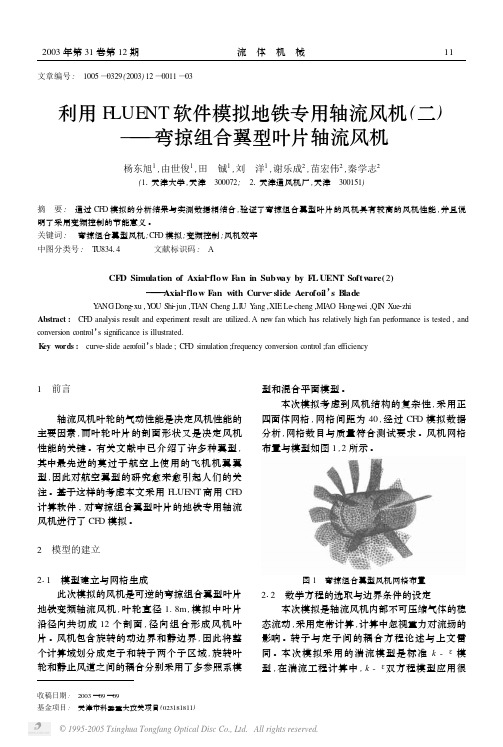
文章编号: 1005—0329(2003)12—0011—03利用F LUENT软件模拟地铁专用轴流风机(二)———弯掠组合翼型叶片轴流风机杨东旭1,由世俊1,田 铖1,刘 洋1,谢乐成2,苗宏伟2,秦学志2(11天津大学,天津 300072; 21天津通风机厂,天津 300151)摘 要: 通过CFD模拟的分析结果与实测数据相结合,验证了弯掠组合翼型叶片的风机具有较高的风机性能,并且说明了采用变频控制的节能意义。
关键词: 弯掠组合翼型风机;CFD模拟;变频控制;风机效率中图分类号: T U83414 文献标识码: ACFD Simulation of Axial2flow F an in Subw ay by F L UENT Softw are(2)———Axial2flow F an with Curve2slide Aerofoil’s B ladeY ANG D ong2xu,Y OU Shi2jun,TI AN Cheng,LI U Y ang,XIE Le2cheng,MI AO H ong2wei,QI N Xue2zhiAbstract: CFD analysis result and experiment result are utilized.A new fan which has relatively high fan performance is tested,and conversion control’s significance is illustrated.K ey w ords: curve2slide aerofoil’s blade;CFD simulation;frequency conversion control;fan efficiency1 前言轴流风机叶轮的气动性能是决定风机性能的主要因素,而叶轮叶片的剖面形状又是决定风机性能的关键。
有关文献中已介绍了许多种翼型,其中最先进的莫过于航空上使用的飞机机翼翼型,因此对航空翼型的研究愈来愈引起人们的关注。
- 1、下载文档前请自行甄别文档内容的完整性,平台不提供额外的编辑、内容补充、找答案等附加服务。
- 2、"仅部分预览"的文档,不可在线预览部分如存在完整性等问题,可反馈申请退款(可完整预览的文档不适用该条件!)。
- 3、如文档侵犯您的权益,请联系客服反馈,我们会尽快为您处理(人工客服工作时间:9:00-18:30)。
详细FLUENT实例讲座翼型计算部门: xxx时间: xxx整理范文,仅供参考,可下载自行编辑CAE联盟论坛精品讲座系列详细FLUENT实例讲座-翼型计算主讲人:流沙 CAE联盟论坛总版主1.1 问题描述翼型升阻力计算是CFD最常规的应用之一。
本例计算的翼型为RAE2822,其几何参数可以查看翼型数据库。
本例计算在来流速度0.75马赫,攻角3.19°情况下,翼型的升阻系数及流场分布,并将计算结果与实验数据进行对比。
模型示意图如图1所示。
b5E2RGbCAP1.png(12.13 K>2018/7/29 23:41:251.2 FLUENT前处理设置Step 1:导入计算模型以3D,双精度方式启动FLUENT14.5。
利用菜单【File】>【Read】>【Mesh…】,在弹出的文件选择对话框中选择网格文件rae2822_coarse.msh,点击OK按钮选择文件。
如图2所示。
p1EanqFDPw点击FLUENT模型树按钮General,在右侧设置面板中点击按钮Display…,在弹出的设置对话框中保持默认设置,点击Display按钮,显示网格。
如图3所示。
DXDiTa9E3d2.png(11.51K>2018/7/29 23:41:253.png(33.41 K>2018/7/29 23:41:253-2.png(52.04 K>2018/7/29 23:41:25Step 2:检查网格采用如图4所示步骤进行网格的检查与显示。
点击FLUENT模型树节点General节点,在右侧面板中通过按钮Scale…、Check及Report Quality实现网格检查。
4.png(12.10 K>RTCrpUDGiT2018/7/29 23:41:25点击按钮Check,在命令输出按钮出现如图5所示网格统计信息。
从图中可以看出,网格尺寸分布:x轴:-48.97~50my轴:0~0.01mz轴:-50~50m符合尺寸要求,无需进行尺寸缩放。
最小网格体积参数minimum volume为1.690412e-9,为大于0的值,符合计算要求。
5.png(27.22 K>2018/7/29 23:41:25Step 3:General设置点击模型树节点General,在右侧设置面板中Solver下设置求解器为Density-Based,如图6所示。
5PCzVD7HxA小提示:对于高速可压缩流场计算,常常使用密度基求解器。
Step 4:Models设置使用SST k-w湍流模型,并且激活能量方程。
1、激活SST k-w湍流模型如图6-7所示,点击模型树节点Models,在右侧面板中的models 列表项中鼠标双击Viscous-laminar,弹出如图6-8所示粘性模型设置对话框,在model选项中选择k-omega(2 eqn>,并在k-omega Model选项中选择选项SST,其它参数保持默认。
jLBHrnAILg小技巧:对于外流场模型,若壁面附近流场非常重要,则SST k-w 模型是理想的选择。
该湍流模型可以求解粘性子层,不过对网格要求较高,壁面附近需要非常细密的网格。
xHAQX74J0X2、激活能量方程在图7所示面板中鼠标双击列表项Eneergy-Off,弹出能量方程设置面板,在面板中激活Energy Equation选项。
8.png(42.49 K>LDAYtRyKfE2018/7/2923:41:25Step 5:Materials设置设置气体密度为理想气体类型。
如图9所示,点击FLUENT模型树节点Materials,在右侧设置面板中选择材料air,点击按钮Create/Edit…,弹出材料设置对话框。
如图10所示。
Zzz6ZB2Ltk设置密度Density选项为ideal-gas,设置粘性Viscosity选项为sutherland,在弹出的相应面板中采取默认设置。
点击Change/Create按钮完成材料属性的编辑。
dvzfvkwMI1小提示:ideal-gas采用的是理想气体状态方程,能够反应压力与密度的关系,可以模拟流体的可压缩性。
对于高速可压缩流动问题,通常其流体物性与温度关系较大,本例进行了简化,设置其比热及热传导率为定值。
rqyn14ZNXIStep 6:Cell Zone Conditions设置在Cell Zone Conditions中设置参考压力为0。
如图11所示,点击模型树节点Cell Zone Conditions,在右侧设置面板中点击按钮Operating Conditions…,弹出如图12所示的设置对话框。
在对话框中设置参数Operating Pressure为0。
EmxvxOtOco小技巧:设置操作压力为零意味着在边界条件中设置的压力均为绝对压力。
Step 7:Boundary Conditions设置设置入口边界inlet的边界类型为Pressure Far-Field。
设置壁面边界airfoil的边界类型为Wall。
设置对称边界symmetry的边界类型为Symmetry。
1、设置入口边界inlet如图13所示,点击模型树节点Boundary Conditions,在右侧面板中Zone选项中选择列表项inlet,设置边界类型Type为pressure-far-field,点击Edit…按钮在弹出的参数设置对话框中设置入口边界参数。
如图14所示。
SixE2yXPq5在Momentum标签页中,设置表压Gauge Pressure为11111Pa,设置马赫数Mach Number为0.75,设置速度向量为直角坐标方式Cartesian。
设置方向向量为<0.99845,0,0.05565)。
该向量为通过攻角3.19°计算获得。
Cos3.19°=0.99845,sin3.19°=0.05565。
6ewMyirQFL设置湍流指定方式Specification Method为Intensity and Viscosity Ratio,指定湍流强度Turbulent Intensity为1%,湍流粘度比Turbulent Viscosity Ratio为1。
kavU42VRUs切换至Thermal标签页,设置温度Temperature为216.65K。
如图15所示。
2、设置airfoil边界及symmetry边界设置airfoil边界类型为Wall,保持参数默认,即使用无滑移光滑绝热壁面。
修改symmetry边界类型为Symmetry。
Step 8:Reference Value设置参考值主要用于升阻系数的计算。
如图16所示设置。
点击模型树节点Reference Values,在右侧面板中Computer from 选择inlet,软件会自动对下方的参数进行填充。
用户需要确保Area参数值为0.01。
y6v3ALoS89软件利用参数值进行升力系数及阻力系数的计算:式中,CD为阻力系数,CL为升力系数。
Fstream为水平分力,Flateral为垂直分力。
Step 9:Solution Methods设置如图17所示,点击模型树节点Solution Methods,在右侧面板中设置求解方法。
如图所示,使用Implicit及Roe-FDS求解方法,修改Turbulent Kinetic Energy与Specific Dissipation Rat为Second Order Upwind,其它参数保持默认设置。
M2ub6vSTnPStep 10:Solution Controls设置求解控制参数采用默认设置。
该面板中的设置主要用于控制收敛性,通常软件会根据用户设置的模型及边界条件对控制参数进行一定的优化,用户往往无需进行设定。
在该面板中主要设置物理量的亚松弛因子。
增大亚松弛因子能提高收敛速度,但是会降低稳定性。
0YujCfmUCwStep 11:Monitor设置可以定义升力及阻力系数监视器,以观察这些物理量随迭代进行的变化情况。
1、定义阻力监视器如图18所示,鼠标点击模型树节点Monitors,在右侧设置面板中点击如图所示Create按钮下的Drag…菜单,弹出如图19所示的设置对话框。
eUts8ZQVRd按如图19所示,定义阻力监视器。
2、升力监视器升力监视器定义步骤与阻力监视器相同,所不同的是力向量Force Vector改为[-0.0556,0,。
sQsAEJkW5TStep 12:Solution Initialization设置以入口inlet边界条件进行初始化。
如图20及图21所示。
Step 13:Run Calculation设置点击FLUENT模型树节点Run Calculation,右侧面板设置如图21所示。
设置Number of Iterations为0,激活选项Solution Steering,在选项Flow Type为Transonic,激活选项Use FMG Initialization,点击按钮Calculate进行FMG初始化。
GMsIasNXkA小技巧:对于航空外流问题,采用FMG初始化有助于提高收敛性。
设置Number of Iterations为900,取消激活选项Use FMG Initialization,点击Calculation按钮进行迭代计算。
TIrRGchYzg1.3 结果后处理Step 1:升阻系数监控曲线图22与图23分别为升力系数与阻力系数监控曲线。
从图中可以看出,随着迭代次数的增加,升力系数及阻力系数逐渐趋于稳定。
可以认为计算达到收敛。
7EqZcWLZNX图24为迭代输出结果部分截图,从图中可以看出,升力系数约为0.71,阻力系数约为0.027416。
Step 2:沿壁面的压力系数分布点击模型树节点Plot,在右侧面板中选择列表项XY Plot,弹出面板如图25所示。
激活选项Node Values与Position on X Axis,设置Plot Direction为<1,0,0),设置Y Axis Function为Pressure与Pressure Coefficient,设置X Axis Function为Direction Vector,选择Surface为airfoil。
lzq7IGf02E点击按钮Load File…,在弹出的文件选择对话框中选择实验数据文件experiment.xy。
点击Plot按钮显示曲线。
压力系数分布如图28所示。
zvpgeqJ1hk点击Axes按钮,弹出如图26所示坐标轴样式设置对话框。
激活选择Y Axis,设置Number Format的Type为float,设置精度Precision为2。