matlab典型例题
matlab编程实例100例
1-32是:图形应用篇33-66是:界面设计篇67-84是:图形处理篇85-100是:数值分析篇实例1:三角函数曲线(1)function shili01h0=figure('toolbar','none',...'position',[198 56 350 300],...'name','实例01');h1=axes('parent',h0,...'visible','off');x=-pi:0.05:pi;y=sin(x);plot(x,y);xlabel('自变量X');ylabel('函数值Y');title('SIN( )函数曲线');grid on实例2:三角函数曲线(2)function shili02h0=figure('toolbar','none',...'position',[200 150 450 350],...'name','实例02');x=-pi:0.05:pi;y=sin(x)+cos(x);plot(x,y,'-*r','linewidth',1);grid onxlabel('自变量X');ylabel('函数值Y');title('三角函数');实例3:图形的叠加function shili03h0=figure('toolbar','none',...'position',[200 150 450 350],...'name','实例03');x=-pi:0.05:pi;y1=sin(x);y2=cos(x);plot(x,y1,...'-*r',...x,y2,...'--og');grid onxlabel('自变量X');ylabel('函数值Y');title('三角函数');实例4:双y轴图形的绘制function shili04h0=figure('toolbar','none',...'position',[200 150 450 250],...'name','实例04');x=0:900;a=1000;b=0.005;y1=2*x;y2=cos(b*x);[haxes,hline1,hline2]=plotyy(x,y1,x,y2,'semilogy','plot'); axes(haxes(1))ylabel('semilog plot');axes(haxes(2))ylabel('linear plot');实例5:单个轴窗口显示多个图形function shili05h0=figure('toolbar','none',...'position',[200 150 450 250],...'name','实例05');t=0:pi/10:2*pi;[x,y]=meshgrid(t);subplot(2,2,1)plot(sin(t),cos(t))axis equalsubplot(2,2,2)z=sin(x)-cos(y);plot(t,z)axis([0 2*pi -2 2])subplot(2,2,3)h=sin(x)+cos(y);plot(t,h)axis([0 2*pi -2 2])subplot(2,2,4)g=(sin(x).^2)-(cos(y).^2);plot(t,g)axis([0 2*pi -1 1])实例6:图形标注function shili06h0=figure('toolbar','none',...'position',[200 150 450 400],...'name','实例06');t=0:pi/10:2*pi;h=plot(t,sin(t));xlabel('t=0到2\pi','fontsize',16);ylabel('sin(t)','fontsize',16);title('\it{从0to2\pi 的正弦曲线}','fontsize',16) x=get(h,'xdata');y=get(h,'ydata');imin=find(min(y)==y);imax=find(max(y)==y);text(x(imin),y(imin),...['\leftarrow最小值=',num2str(y(imin))],...'fontsize',16)text(x(imax),y(imax),...['\leftarrow最大值=',num2str(y(imax))],...'fontsize',16)实例7:条形图形function shili07h0=figure('toolbar','none',...'position',[200 150 450 350],...'name','实例07');tiao1=[562 548 224 545 41 445 745 512];tiao2=[47 48 57 58 54 52 65 48];t=0:7;bar(t,tiao1)xlabel('X轴');ylabel('TIAO1值');h1=gca;h2=axes('position',get(h1,'position'));plot(t,tiao2,'linewidth',3)set(h2,'yaxislocation','right','color','none','xticklabel',[]) 实例8:区域图形function shili08h0=figure('toolbar','none',...'position',[200 150 450 250],...'name','实例08');x=91:95;profits1=[88 75 84 93 77];profits2=[51 64 54 56 68];profits3=[42 54 34 25 24];profits4=[26 38 18 15 4];area(x,profits1,'facecolor',[0.5 0.9 0.6],...'edgecolor','b',...'linewidth',3)hold onarea(x,profits2,'facecolor',[0.9 0.85 0.7],...'edgecolor','y',...'linewidth',3)hold onarea(x,profits3,'facecolor',[0.3 0.6 0.7],...'edgecolor','r',...'linewidth',3)hold onarea(x,profits4,'facecolor',[0.6 0.5 0.9],...'edgecolor','m',...'linewidth',3)hold offset(gca,'xtick',[91:95])set(gca,'layer','top')gtext('\leftarrow第一季度销量')gtext('\leftarrow第二季度销量')gtext('\leftarrow第三季度销量')gtext('\leftarrow第四季度销量')xlabel('年','fontsize',16);ylabel('销售量','fontsize',16);实例9:饼图的绘制function shili09h0=figure('toolbar','none',...'position',[200 150 450 250],...'name','实例09');t=[54 21 35;68 54 35;45 25 12;48 68 45;68 54 69];x=sum(t);h=pie(x);textobjs=findobj(h,'type','text');str1=get(textobjs,{'string'});val1=get(textobjs,{'extent'});oldext=cat(1,val1{:});names={'商品一:';'商品二:';'商品三:'};str2=strcat(names,str1);set(textobjs,{'string'},str2)val2=get(textobjs,{'extent'});newext=cat(1,val2{:});offset=sign(oldext(:,1)).*(newext(:,3)-oldext(:,3))/2; pos=get(textobjs,{'position'});textpos=cat(1,pos{:});textpos(:,1)=textpos(:,1)+offset;set(textobjs,{'position'},num2cell(textpos,[3,2]))实例10:阶梯图function shili10h0=figure('toolbar','none',...'position',[200 150 450 400],...'name','实例10');a=0.01;b=0.5;t=0:10;f=exp(-a*t).*sin(b*t);stairs(t,f)hold onplot(t,f,':*')hold offglabel='函数e^{-(\alpha*t)}sin\beta*t的阶梯图'; gtext(glabel,'fontsize',16)xlabel('t=0:10','fontsize',16)axis([0 10 -1.2 1.2])实例11:枝干图function shili11h0=figure('toolbar','none',...'position',[200 150 450 350],...'name','实例11');x=0:pi/20:2*pi;y1=sin(x);y2=cos(x);h1=stem(x,y1+y2);hold onh2=plot(x,y1,'^r',x,y2,'*g');hold offh3=[h1(1);h2];legend(h3,'y1+y2','y1=sin(x)','y2=cos(x)') xlabel('自变量X');ylabel('函数值Y');title('正弦函数与余弦函数的线性组合');实例12:罗盘图function shili12h0=figure('toolbar','none',...'position',[200 150 450 250],...'name','实例12');winddirection=[54 24 65 84256 12 235 62125 324 34 254];windpower=[2 5 5 36 8 12 76 14 10 8];rdirection=winddirection*pi/180;[x,y]=pol2cart(rdirection,windpower); compass(x,y);desc={'风向和风力','气象台','10月1日0:00到','10月1日12:00'};gtext(desc)实例13:轮廓图function shili13h0=figure('toolbar','none',...'position',[200 150 450 250],...'name','实例13');[th,r]=meshgrid((0:10:360)*pi/180,0:0.05:1); [x,y]=pol2cart(th,r);z=x+i*y;f=(z.^4-1).^(0.25);contour(x,y,abs(f),20)axis equalxlabel('实部','fontsize',16);ylabel('虚部','fontsize',16);h=polar([0 2*pi],[0 1]);delete(h)hold oncontour(x,y,abs(f),20)实例14:交互式图形function shili14h0=figure('toolbar','none',...'position',[200 150 450 250],...'name','实例14');axis([0 10 0 10]);hold onx=[];y=[];n=0;disp('单击鼠标左键点取需要的点'); disp('单击鼠标右键点取最后一个点'); but=1;while but==1[xi,yi,but]=ginput(1);plot(xi,yi,'bo')n=n+1;disp('单击鼠标左键点取下一个点');x(n,1)=xi;y(n,1)=yi;endt=1:n;ts=1:0.1:n;xs=spline(t,x,ts);ys=spline(t,y,ts);plot(xs,ys,'r-');hold off实例14:交互式图形function shili14h0=figure('toolbar','none',...'position',[200 150 450 250],...'name','实例14');axis([0 10 0 10]);hold onx=[];y=[];n=0;disp('单击鼠标左键点取需要的点'); disp('单击鼠标右键点取最后一个点'); but=1;while but==1[xi,yi,but]=ginput(1);plot(xi,yi,'bo')n=n+1;disp('单击鼠标左键点取下一个点');x(n,1)=xi;y(n,1)=yi;endt=1:n;ts=1:0.1:n;xs=spline(t,x,ts);ys=spline(t,y,ts);plot(xs,ys,'r-');hold off实例15:变换的傅立叶函数曲线function shili15h0=figure('toolbar','none',...'position',[200 150 450 250],...'name','实例15');axis equalm=moviein(20,gcf);set(gca,'nextplot','replacechildren') h=uicontrol('style','slider','position',...[100 10 500 20],'min',1,'max',20) for j=1:20plot(fft(eye(j+16)))set(h,'value',j)m(:,j)=getframe(gcf);endclf;axes('position',[0 0 1 1]);movie(m,30)实例16:劳伦兹非线形方程的无序活动function shili15h0=figure('toolbar','none',...'position',[200 150 450 250],...'name','实例15');axis equalm=moviein(20,gcf);set(gca,'nextplot','replacechildren') h=uicontrol('style','slider','position',...[100 10 500 20],'min',1,'max',20) for j=1:20plot(fft(eye(j+16)))set(h,'value',j)m(:,j)=getframe(gcf);endclf;axes('position',[0 0 1 1]);movie(m,30)实例17:填充图function shili17h0=figure('toolbar','none',...'position',[200 150 450 250],...'name','实例17');t=(1:2:15)*pi/8;x=sin(t);y=cos(t);fill(x,y,'r')axis square offtext(0,0,'STOP',...'color',[1 1 1],...'fontsize',50,...'horizontalalignment','center') 例18:条形图和阶梯形图function shili18h0=figure('toolbar','none',...'position',[200 150 450 250],...'name','实例18');subplot(2,2,1)x=-3:0.2:3;y=exp(-x.*x);bar(x,y)title('2-D Bar Chart')subplot(2,2,2)x=-3:0.2:3;y=exp(-x.*x);bar3(x,y,'r')title('3-D Bar Chart')subplot(2,2,3)x=-3:0.2:3;y=exp(-x.*x);stairs(x,y)title('Stair Chart')subplot(2,2,4)x=-3:0.2:3;y=exp(-x.*x);barh(x,y)title('Horizontal Bar Chart')实例19:三维曲线图function shili19h0=figure('toolbar','none',...'position',[200 150 450 400],...'name','实例19');subplot(2,1,1)x=linspace(0,2*pi);y1=sin(x);y2=cos(x);y3=sin(x)+cos(x);z1=zeros(size(x));z2=0.5*z1;z3=z1;plot3(x,y1,z1,x,y2,z2,x,y3,z3)grid onxlabel('X轴');ylabel('Y轴');zlabel('Z轴');title('Figure1:3-D Plot')subplot(2,1,2)x=linspace(0,2*pi);y1=sin(x);y2=cos(x);y3=sin(x)+cos(x);z1=zeros(size(x));z2=0.5*z1;z3=z1;plot3(x,z1,y1,x,z2,y2,x,z3,y3)grid onxlabel('X轴');ylabel('Y轴');zlabel('Z轴');title('Figure2:3-D Plot')实例20:图形的隐藏属性function shili20h0=figure('toolbar','none',...'position',[200 150 450 300],...'name','实例20');subplot(1,2,1)[x,y,z]=sphere(10);mesh(x,y,z)axis offtitle('Figure1:Opaque')hidden onsubplot(1,2,2)[x,y,z]=sphere(10);mesh(x,y,z)axis offtitle('Figure2:Transparent') hidden off实例21PEAKS函数曲线function shili21h0=figure('toolbar','none',...'position',[200 100 450 450],...'name','实例21');[x,y,z]=peaks(30);subplot(2,1,1)x=x(1,:);y=y(:,1);i=find(y>0.8&y<1.2);j=find(x>-0.6&x<0.5);z(i,j)=nan*z(i,j);surfc(x,y,z)xlabel('X轴');ylabel('Y轴');zlabel('Z轴');title('Figure1:surfc函数形成的曲面') subplot(2,1,2)x=x(1,:);y=y(:,1);i=find(y>0.8&y<1.2);j=find(x>-0.6&x<0.5);z(i,j)=nan*z(i,j);surfl(x,y,z)xlabel('X轴');ylabel('Y轴');zlabel('Z轴');title('Figure2:surfl函数形成的曲面')实例22:片状图function shili22h0=figure('toolbar','none',...'position',[200 150 550 350],...'name','实例22');subplot(1,2,1)x=rand(1,20);y=rand(1,20);z=peaks(x,y*pi);t=delaunay(x,y);trimesh(t,x,y,z)hidden offtitle('Figure1:Triangular Surface Plot'); subplot(1,2,2)x=rand(1,20);y=rand(1,20);z=peaks(x,y*pi);t=delaunay(x,y);trisurf(t,x,y,z)title('Figure1:Triangular Surface Plot'); 实例23:视角的调整function shili23h0=figure('toolbar','none',...'position',[200 150 450 350],...'name','实例23');x=-5:0.5:5;[x,y]=meshgrid(x);r=sqrt(x.^2+y.^2)+eps;z=sin(r)./r;subplot(2,2,1)surf(x,y,z)xlabel('X-axis')ylabel('Y-axis')zlabel('Z-axis')title('Figure1')view(-37.5,30)subplot(2,2,2)surf(x,y,z)xlabel('X-axis')ylabel('Y-axis')zlabel('Z-axis')title('Figure2')view(-37.5+90,30)subplot(2,2,3)surf(x,y,z)xlabel('X-axis')ylabel('Y-axis')zlabel('Z-axis')title('Figure3')view(-37.5,60)subplot(2,2,4)surf(x,y,z)xlabel('X-axis')ylabel('Y-axis')zlabel('Z-axis')title('Figure4')view(180,0)实例24:向量场的绘制function shili24h0=figure('toolbar','none',...'position',[200 150 450 350],...'name','实例24');subplot(2,2,1)z=peaks;ribbon(z)title('Figure1')subplot(2,2,2)[x,y,z]=peaks(15);[dx,dy]=gradient(z,0.5,0.5); contour(x,y,z,10)hold onquiver(x,y,dx,dy)hold offtitle('Figure2')subplot(2,2,3)[x,y,z]=peaks(15);[nx,ny,nz]=surfnorm(x,y,z);surf(x,y,z)hold onquiver3(x,y,z,nx,ny,nz)hold offtitle('Figure3')subplot(2,2,4)x=rand(3,5);y=rand(3,5);z=rand(3,5);c=rand(3,5);fill3(x,y,z,c)grid ontitle('Figure4')实例25:灯光定位function shili25h0=figure('toolbar','none',...'position',[200 150 450 250],...'name','实例25');vert=[1 1 1;1 2 1;2 2 1;2 1 1;1 1 2;12 2;2 2 2;2 1 2];fac=[1 2 3 4;2 6 7 3;4 3 7 8;15 8 4;1 2 6 5;5 6 7 8];grid offsphere(36)h=findobj('type','surface');set(h,'facelighting','phong',...'facecolor',...'interp',...'edgecolor',[0.4 0.4 0.4],...'backfacelighting',...'lit')hold onpatch('faces',fac,'vertices',vert,...'facecolor','y');light('position',[1 3 2]);light('position',[-3 -1 3]); material shinyaxis vis3d offhold off实例26:柱状图function shili26h0=figure('toolbar','none',...'position',[200 50 450 450],...'name','实例26');subplot(2,1,1)x=[5 2 18 7 39 8 65 5 54 3 2];bar(x)xlabel('X轴');ylabel('Y轴');title('第一子图');subplot(2,1,2)y=[5 2 18 7 39 8 65 5 54 3 2];barh(y)xlabel('X轴');ylabel('Y轴');title('第二子图');实例27:设置照明方式function shili27h0=figure('toolbar','none',...'position',[200 150 450 350],...'name','实例27');subplot(2,2,1)sphereshading flatcamlight leftcamlight rightlighting flatcolorbaraxis offtitle('Figure1')subplot(2,2,2)sphereshading flatcamlight leftcamlight rightlighting gouraudcolorbaraxis offtitle('Figure2')subplot(2,2,3)sphereshading interpcamlight rightcamlight leftlighting phongcolorbaraxis offtitle('Figure3')subplot(2,2,4)sphereshading flatcamlight leftcamlight rightlighting nonecolorbaraxis offtitle('Figure4')实例28:羽状图function shili28h0=figure('toolbar','none',...'position',[200 150 450 350],...'name','实例28');subplot(2,1,1)alpha=90:-10:0;r=ones(size(alpha));m=alpha*pi/180;n=r*10;[u,v]=pol2cart(m,n);feather(u,v)title('羽状图')axis([0 20 0 10])subplot(2,1,2)t=0:0.5:10;x=0.05+i;y=exp(-x*t);feather(y)title('复数矩阵的羽状图')实例29:立体透视(1)function shili29h0=figure('toolbar','none',...'position',[200 150 450 250],...'name','实例29');[x,y,z]=meshgrid(-2:0.1:2,...-2:0.1:2,...-2:0.1:2);v=x.*exp(-x.^2-y.^2-z.^2);grid onfor i=-2:0.5:2;h1=surf(linspace(-2,2,20),...linspace(-2,2,20),...zeros(20)+i);rotate(h1,[1 -1 1],30)dx=get(h1,'xdata');dy=get(h1,'ydata');dz=get(h1,'zdata');delete(h1)slice(x,y,z,v,[-2 2],2,-2)hold onslice(x,y,z,v,dx,dy,dz)hold offaxis tightview(-5,10)drawnowend实例30:立体透视(2)function shili30h0=figure('toolbar','none',...'position',[200 150 450 250],...'name','实例30');[x,y,z]=meshgrid(-2:0.1:2,...-2:0.1:2,...-2:0.1:2);v=x.*exp(-x.^2-y.^2-z.^2); [dx,dy,dz]=cylinder;slice(x,y,z,v,[-2 2],2,-2)for i=-2:0.2:2h=surface(dx+i,dy,dz);rotate(h,[1 0 0],90)xp=get(h,'xdata');yp=get(h,'ydata');zp=get(h,'zdata');delete(h)hold onhs=slice(x,y,z,v,xp,yp,zp);axis tightxlim([-3 3])view(-10,35)drawnowdelete(hs)hold offend实例31:表面图形function shili31h0=figure('toolbar','none',...'position',[200 150 550 250],...'name','实例31');subplot(1,2,1)x=rand(100,1)*16-8;y=rand(100,1)*16-8;r=sqrt(x.^2+y.^2)+eps;z=sin(r)./r;xlin=linspace(min(x),max(x),33); ylin=linspace(min(y),max(y),33); [X,Y]=meshgrid(xlin,ylin);Z=griddata(x,y,z,X,Y,'cubic'); mesh(X,Y,Z)axis tighthold onplot3(x,y,z,'.','Markersize',20)subplot(1,2,2)k=5;n=2^k-1;theta=pi*(-n:2:n)/n;phi=(pi/2)*(-n:2:n)'/n;X=cos(phi)*cos(theta);Y=cos(phi)*sin(theta);Z=sin(phi)*ones(size(theta));colormap([0 0 0;1 1 1])C=hadamard(2^k);surf(X,Y,Z,C)axis square实例32:沿曲线移动的小球h0=figure('toolbar','none',...'position',[198 56 408 468],...'name','实例32');h1=axes('parent',h0,...'position',[0.15 0.45 0.7 0.5],...'visible','on');t=0:pi/24:4*pi;y=sin(t);plot(t,y,'b')n=length(t);h=line('color',[0 0.5 0.5],...'linestyle','.',...'markersize',25,...'erasemode','xor');k1=uicontrol('parent',h0,...'style','pushbutton',...'position',[80 100 50 30],...'string','开始',...'callback',[...'i=1;',...'k=1;,',...'m=0;,',...'while 1,',...'if k==0,',...'break,',...'end,',...'if k~=0,',...'set(h,''xdata'',t(i),''ydata'',y(i)),',...'drawnow;,',...'i=i+1;,',...'if i>n,',...'m=m+1;,',...'i=1;,',...'end,',...'end,',...'end']);k2=uicontrol('parent',h0,...'style','pushbutton',...'position',[180 100 50 30],...'string','停止',...'callback',[...'k=0;,',...'set(e1,''string'',m),',...'p=get(h,''xdata'');,',...'q=get(h,''ydata'');,',...'set(e2,''string'',p);,',...'set(e3,''string'',q)']); k3=uicontrol('parent',h0,...'style','pushbutton',...'position',[280 100 50 30],...'string','关闭',...'callback','close');e1=uicontrol('parent',h0,...'style','edit',...'position',[60 30 60 20]);t1=uicontrol('parent',h0,...'style','text',...'string','循环次数',...'position',[60 50 60 20]);e2=uicontrol('parent',h0,...'style','edit',...'position',[180 30 50 20]); t2=uicontrol('parent',h0,...'style','text',...'string','终点的X坐标值',...'position',[155 50 100 20]); e3=uicontrol('parent',h0,...'style','edit',...'position',[300 30 50 20]); t3=uicontrol('parent',h0,...'style','text',...'string','终点的Y坐标值',...'position',[275 50 100 20]);实例33:曲线转换按钮h0=figure('toolbar','none',...'position',[200 150 450 250],...'name','实例33');x=0:0.5:2*pi;y=sin(x);h=plot(x,y);grid onhuidiao=[...'if i==1,',...'i=0;,',...'y=cos(x);,',...'delete(h),',...'set(hm,''string'',''正弦函数''),',...'h=plot(x,y);,',...'grid on,',...'else if i==0,',...'i=1;,',...'y=sin(x);,',...'set(hm,''string'',''余弦函数''),',...'delete(h),',...'h=plot(x,y);,',...'grid on,',...'end,',...'end'];hm=uicontrol(gcf,'style','pushbutton',...'string','余弦函数',...'callback',huidiao);i=1;set(hm,'position',[250 20 60 20]);set(gca,'position',[0.2 0.2 0.6 0.6])title('按钮的使用')hold on实例34:栅格控制按钮h0=figure('toolbar','none',...'position',[200 150 450 250],...'name','实例34');x=0:0.5:2*pi;y=sin(x);plot(x,y)huidiao1=[...'set(h_toggle2,''value'',0),',...'grid on,',...];huidiao2=[...'set(h_toggle1,''value'',0),',...'grid off,',...];h_toggle1=uicontrol(gcf,'style','togglebutton',...'string','grid on',...'value',0,...'position',[20 45 50 20],...'callback',huidiao1);h_toggle2=uicontrol(gcf,'style','togglebutton',...'string','grid off',...'value',0,...'position',[20 20 50 20],...'callback',huidiao2);set(gca,'position',[0.2 0.2 0.6 0.6])title('开关按钮的使用')实例35:编辑框的使用h0=figure('toolbar','none',...'position',[200 150 350 250],...'name','实例35');f='Please input the letter';huidiao1=[...'g=upper(f);,',...'set(h2_edit,''string'',g),',...];huidiao2=[...'g=lower(f);,',...'set(h2_edit,''string'',g),',...];h1_edit=uicontrol(gcf,'style','edit',...'position',[100 200 100 50],...'HorizontalAlignment','left',...'string','Please input the letter',...'callback','f=get(h1_edit,''string'');',...'background','w',...'max',5,...'min',1);h2_edit=uicontrol(gcf,'style','edit',...'HorizontalAlignment','left',...'position',[100 100 100 50],...'max',5,...'min',1);h1_button=uicontrol(gcf,'style','pushbutton',...'string','小写变大写',...'position',[100 45 100 20],...'callback',huidiao1);h2_button=uicontrol(gcf,'style','pushbutton',...'string','大写变小写',...'position',[100 20 100 20],...'callback',huidiao2);实例36:弹出式菜单h0=figure('toolbar','none',...'position',[200 150 450 250],...'name','实例36');x=0:0.5:2*pi;y=sin(x);h=plot(x,y);grid onhm=uicontrol(gcf,'style','popupmenu',...'string',...'sin(x)|cos(x)|sin(x)+cos(x)|exp(-sin(x))',...'position',[250 20 50 20]);set(hm,'value',1)huidiao=[...'v=get(hm,''value'');,',...'switch v,',...'case 1,',...'delete(h),',...'y=sin(x);,',...'h=plot(x,y);,',...'grid on,',...'case 2,',...'delete(h),',...'y=cos(x);,',...'h=plot(x,y);,',...'grid on,',...'case 3,',...'delete(h),',...'y=sin(x)+cos(x);,',...'h=plot(x,y);,',...'grid on,',...'case 4,',...'y=exp(-sin(x));,',...'h=plot(x,y);,',...'grid on,',...'end'];set(hm,'callback',huidiao)set(gca,'position',[0.2 0.2 0.6 0.6])title('弹出式菜单的使用')实例37:滑标的使用h0=figure('toolbar','none',...'position',[200 150 450 250],...'name','实例37');[x,y]=meshgrid(-8:0.5:8);r=sqrt(x.^2+y.^2)+eps;z=sin(r)./r;h0=mesh(x,y,z);h1=axes('position',...[0.2 0.2 0.5 0.5],...'visible','off');htext=uicontrol(gcf,...'units','points',...'position',[20 30 45 15],...'string','brightness',...'style','text');hslider=uicontrol(gcf,...'units','points',...'position',[10 10 300 15],...'min',-1,...'max',1,...'style','slider',...'callback',...'brighten(get(hslider,''value''))');实例38:多选菜单h0=figure('toolbar','none',...'position',[200 150 450 250],...'name','实例38');[x,y]=meshgrid(-8:0.5:8);r=sqrt(x.^2+y.^2)+eps;z=sin(r)./r;h0=mesh(x,y,z);hlist=uicontrol(gcf,'style','listbox',...'string','default|spring|summer|autumn|winter',...'max',5,...'min',1,...'position',[20 20 80 100],...'callback',[...'k=get(hlist,''value'');,',...'switch k,',...'case 1,',...'colormap default,',...'case 2,',...'colormap spring,',...'case 3,',...'colormap summer,',...'case 4,',...'colormap autumn,',...'case 5,',...'colormap winter,',...'end']);实例39:菜单控制的使用h0=figure('toolbar','none',...'position',[200 150 450 250],...'name','实例39');x=0:0.5:2*pi;y=cos(x);h=plot(x,y);grid onset(gcf,'toolbar','none')hm=uimenu('label','example');huidiao1=[...'set(hm_gridon,''checked'',''on''),',...'set(hm_gridoff,''checked'',''off''),',...'grid on'];huidiao2=[...'set(hm_gridoff,''checked'',''on''),',...'set(hm_gridon,''checked'',''off''),',...'grid off'];hm_gridon=uimenu(hm,'label','grid on',...'checked','on',...'callback',huidiao1);hm_gridoff=uimenu(hm,'label','grid off',...'checked','off',...'callback',huidiao2);实例40:UIMENU菜单的应用。
MATLAB习题及参考答案经典.doc
习题:1, 计算⎥⎦⎤⎢⎣⎡=572396a 与⎥⎦⎤⎢⎣⎡=864142b 的数组乘积。
2, 对于B AX =,如果⎥⎥⎥⎦⎤⎢⎢⎢⎣⎡=753467294A ,⎥⎥⎥⎦⎤⎢⎢⎢⎣⎡=282637B ,求解X 。
3, 已知:⎥⎥⎥⎦⎤⎢⎢⎢⎣⎡=987654321a ,分别计算a 的数组平方和矩阵平方,并观察其结果。
4, 角度[]604530=x ,求x 的正弦、余弦、正切和余切。
(应用sin,cos,tan.cot)5, 将矩阵⎥⎦⎤⎢⎣⎡=7524a 、⎥⎦⎤⎢⎣⎡=3817b 和⎥⎦⎤⎢⎣⎡=2695c 组合成两个新矩阵: (1)组合成一个4⨯3的矩阵,第一列为按列顺序排列的a 矩阵元素,第二列为按列顺序排列的b 矩阵元素,第三列为按列顺序排列的c 矩阵元素,即 ⎥⎥⎥⎥⎦⎤⎢⎢⎢⎢⎣⎡237912685574(2)按照a 、b 、c 的列顺序组合成一个行矢量,即 []2965318772546, 将(x -6)(x -3)(x -8)展开为系数多项式的形式。
(应用poly,polyvalm)7, 求解多项式x 3-7x 2+2x +40的根。
(应用roots)8, 求解在x =8时多项式(x -1)(x -2) (x -3)(x -4)的值。
(应用poly,polyvalm)9, 计算多项式9514124234++--x x x x 的微分和积分。
(应用polyder,polyint ,poly2sym)10, 解方程组⎥⎥⎥⎦⎤⎢⎢⎢⎣⎡=⎥⎥⎥⎦⎤⎢⎢⎢⎣⎡66136221143092x 。
(应用x=a\b)11, 求欠定方程组⎥⎦⎤⎢⎣⎡=⎥⎦⎤⎢⎣⎡5865394742x 的最小范数解。
(应用pinv) 12, 矩阵⎥⎥⎥⎦⎤⎢⎢⎢⎣⎡-=943457624a ,计算a 的行列式和逆矩阵。
(应用det,inv)13, y =sin(x ),x 从0到2π,∆x =0.02π,求y 的最大值、最小值、均值和标准差。
matlab程序设计例题及答案
matlab程序设计例题及答案1.编写程序:计算1/3+2/5+3/7+……+10/21法一: s=0;for i=1:10s=s+i/(2*i+1); end ss =法二:sum((1:10)./(3:2:21)) ans =2.编写程序:计算1~100中即能被3整除,又能被7整除的所有数之和。
s=0;for i=1:100if mod(i,3)==0&&mod(i,7)==0 s=s+i; end,end ss =2103.画出y=n!的图,阶乘的函数自己编写,禁用MATLAB 自带的阶乘函数。
x=1:10; for i=1:10try y(i)=y(i-1)*i; catch y(i)=1; end,end plot(x,y)106123456789104.一个数恰好等于它的因子之和,这个数就称为完数。
例如,6的因子为1,2,3,而6=1+2+3,因此6就是一个完数。
编程找出20XX以内的所有完数。
g=;for n=2:20XX s=0;for r=1:n-1if mod(n,r)==0 s=s+r; end endif s==ng=[g n]; end end gg =6 28 4965.编写一个函数,模拟numel函数的功能,函数中调用size函数。
function y=numelnumel(x) m=size(x); y=m(1)*m(2);numelnumel([1 2 3;4 5 6])ans =66. 编写一个函数,模拟length函数的功能,函数中调用size函数。
function y=lengthlength(x) m=size(x);y=max(m(1),m(2));lengthlength([1 2 3;4 5 6])ans =37.求矩阵rand的所有元素和及各行平均值,各列平均值。
s=rand(5);sum=sum(sum(s)) mean2=mean(s,2) mean1=mean(s)sum =mean2 =mean1 =8.编程判断1001,1003,1007,1009,1011为素数,若不是,输出其约数。
matlab的例题
浅议matlab 的功能和应用数值计算1、编程求满足∑=>mi i 1100002的最小m 值。
解:m=1; s=0;while s<=10000s=s+2^m; m=m+1;end m=m-1;di sp('m=');disp(m);运行结果:m=132、编写一个函数,计算下面函数的值,给出标量x 的值,调用该函数后,返回y 的值。
function [y]=myfun1(x)选择一些数据测试你编写的函数。
function y=myfun1(x) if x<=0y=sin(x); elseif x>0&x<=3 y=x; else y=6-x; end⎪⎩⎪⎨⎧>+-≤<≤=3,630,0,sin )(x x x x x x x yreturn ;3、编写一个函数,给出一个向量],,[21n x x x x=,生成如下范德蒙矩阵。
function [v]=myvander(x)⎥⎥⎥⎥⎥⎥⎦⎤⎢⎢⎢⎢⎢⎢⎣⎡---112112222121111n n n n n n x x x x x x x x x例如:>>v=myvander([2 3 4 5]) 得v=⎥⎥⎥⎥⎦⎤⎢⎢⎢⎢⎣⎡1256427825169454321111 生成一些数据测试你写的函数。
function [v]=myvander(x) n=length(x); v(1:n)=1; for i=n+1:n*n a=i/n;r=mod(i,n); b=floor(a); if r==0 r=n; b=b-1; endv(i)=x(r)^b; endv=reshape(v,n,n)';>> myvander([1 2 3])ans =1 1 11 2 3 1 4 9>> myvander([ 1 4 6 8])ans =1 1 1 1 1 4 6 8 1 16 36 64 1 64 216 512图像的绘制1、在同一坐标系下绘制下面三个函数在t ∈[0,4π]的图象。
matlab20道试题及解答
试题1.“数学黑洞”:任意一个4位自然数,将组成该数的各位数字重新排列,形成一个最大数和一个最小数,之后两数相减,其差仍为一个自然数。
重复进行上述运算,最终会出现一个神秘的数,请编程输出这个神秘的数。
clear;a=input('请输入一个四位正整数:');str_a=num2str(a); %将a转化为一个字符串b_min=str2double(sort(str_a)); %形成最小数b_max=str2double(sort(str_a,'descend')); %形成最大数b=b_max-b_min; %求最大数与最小数之差while (b~=a)a=b;str_a=num2str(a); %将a转化为一个字符串b_min=str2double(sort(str_a)); %形成最小数b_max=str2double(sort(str_a,'descend')); %形成最大数b=b_max-b_min; %求最大数与最小数之差endb试题2.将数字1、2、3、4、5、6填入一个2行3列的表格中,要使得每一列右边的数字比左边的数字大,每一行下面的数字比上面的数字大。
请编写程序求出按此要求可有几种填写方法。
a(1)=1;a(6)=6;count=0; %用来计数b=perms('2345'); %产生2345的全排列[m,n]=size(b);for i=1:mtemp=b(i,:);a(2)=str2double(temp(1));a(3)=str2double(temp(2));a(4)=str2double(temp(3));a(5)=str2double(temp(4));if ((a(4)>a(2))&&(a(4)>a(3))&&(a(5)>a(3)))count=count+1;c=reshape(a,2,3); %将a向量转化为2*3矩阵输出disp(c);endenddisp(['共有',num2str(count),'种填写方法']); %输出填写方法的种数试题3.编写成绩排序程序。
matlab 程序设计 例题

一、概述Matlab是一种强大的工程计算软件,在工程领域有着广泛的应用。
对于学习Matlab程序设计来说,通过例题学习是非常有效的方法。
通过实际的例题练习,可以帮助学生更深入地理解Matlab的基本原理和应用技巧。
本文将介绍几个常见的Matlab程序设计例题,并进行详细的分析和讲解,希望能够帮助读者加深对Matlab程序设计的理解。
二、例题一:矩阵运算题目:编写一个Matlab程序,实现两个任意大小的矩阵相加的运算。
1.我们需要定义两个任意大小的矩阵A和矩阵B,可以通过rand函数生成随机矩阵,也可以手动输入矩阵的元素。
2.编写Matlab程序,使用矩阵的加法运算符“+”进行矩阵相加操作。
3.输出矩阵相加的结果,并进行验证和检查。
通过这个例题,可以加深对Matlab矩阵运算的理解,包括矩阵的定义、矩阵相加的操作和结果输出的方法。
三、例题二:函数绘图题目:编写一个Matlab程序,绘制sin函数的曲线图像。
1.我们需要定义sin函数的自变量范围和取值步长,可以使用linspace函数生成自变量的取值范围。
2.编写Matlab程序,调用sin函数计算自变量对应的函数值。
3.接下来,使用plot函数绘制sin函数的曲线图像,并设置图像的标题、坐标轴标签等其他参数。
4.输出绘制好的sin函数曲线图像,并进行观察和分析。
通过这个例题,可以了解Matlab中函数绘图的基本方法,包括自变量的定义、函数值的计算和图像的绘制等操作。
四、例题三:数值积分题目:编写一个Matlab程序,实现对指定函数在指定区间上的数值积分。
1.我们需要定义积分的目标函数和积分区间,在Matlab中可以使用function定义目标函数,也可以手动输入目标函数和积分区间。
2.编写Matlab程序,调用Matlab内置的数值积分函数(如quad、quadl等)进行数值积分的计算。
3.输出数值积分的结果,并与解析解进行比较和分析。
通过这个例题,可以了解Matlab中数值积分的计算方法,包括目标函数的定义、积分区间的设定和数值积分函数的调用。
matLAB经典例题及答案
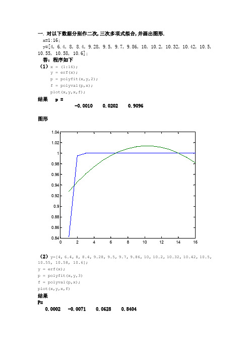
一.对以下数据分别作二次,三次多项式拟合,并画出图形.x=1:16;y=[4,6.4,8,8.4,9.28,9.5,9.7,9.86,10,10.2,10.32,10.42,10.5, 10.55,10.58,10.6];答:程序如下(1)x=(1:16);y=erf(x);p=polyfit(x,y,2);f=polyval(p,x);plot(x,y,x,f);结果p=-0.00100.02020.9096(2)y=[4,6.4,8,8.4,9.28,9.5,9.7,9.86,10,10.2,10.32,10.42,10.5, 10.55,10.58,10.6];y=erf(x);p=polyfit(x,y,3)f=polyval(p,x);plot(x,y,x,f)结果P=0.0002-0.00710.06280.8404二.在[0,4pi]画sin(x),cos(x)(在同一个图象中);其中cos(x)图象用红色小圆圈画.并在函数图上标注“y=sin(x)”,“y=cos(x)”,x轴,y轴,标题为“正弦余弦函数图象”.答:程序如下x=[0:720]*pi/180;plot(x,sin(x),x,cos(x),'ro');x=[2.5;7];y=[0;0];s=['y=sin(x)';'y=cos(x)'];text(x,y,s);xlabel('正弦余弦函数图象'),ylabel('正弦余弦函数图象')图形如下三.选择一个单自由度线性振动系统模型,自定质量、弹簧刚度、阻尼、激振力等一组参数,分别编程(m 文件)计算自由和强迫振动时的响应,并画出振动曲线图。
(要求画出该单自由度线性振动系统模型图)其中质量为m=1000kg,弹性刚度k=48020N/m,阻尼c=1960N.s/m,激振力f(t)=0.阻尼比ζ的程序p=1960/(2*sqrt(48020*1000))求得p=0.1414而p为阻尼比ζ强迫振动时的响应程序g =tf([-101],[48020048020*1.9848020]);bode(g)图形g =tf([001],[0001]);bode(g)振动曲线图程序:函数文件function dx =rigid(t,x)dx =zeros(2,1);dx(1)=x(2);dx(2)=(-48020*x(1)-1960*x(2))/1000;命令文件options =odeset('RelTol',1e-4,'AbsTol',[1e-41e-4]);[T,X]=ode45(@rigid,[012],[11],options);plot(T,X(:,1),'-')其图形如下024681012-6-5-4-3-2-11234单自由度线性强迫振动系统模型图其中质量为m=1000kg,弹性刚度k=48020N/m,阻尼c=1960N.s/m,f(t)=cos(3*pi*t)振动曲线图程序:函数文件function dx=rigid(t,x)dx=zeros(2,1);dx(1)=x(2);dx(2)=(-48020*x(1)-1960*x(2))/1000+cos(3*pi*t);命令文件options=odeset('RelTol',1e-4,'AbsTol',[1e-41e-4]);[T,X]=ode45(@rigid,[020],[11],options);plot(T,X(:,1),'-')力等一组参数,建立Simulink仿真模型框图进行仿真分析。
matlab经典编程例题
以下各题均要求编程实现,并将程序贴在题目下方。
1.从键盘输入任意个正整数,以0结束,输出那些正整数中的素数。
clc;clear;zzs(1)=input('请输入正整数:');k=1;n=0;%素数个数while zzs(k)~=0flag=0;%是否是素数,是则为1for yz=2:sqrt(zzs(k))%因子从2至此数平方根if mod(zzs(k),yz)==0flag=1;break;%非素数跳出循环endendif flag==0&zzs(k)>1%忽略0和1的素数n=n+1;sus(n)=zzs(k);endk=k+1;zzs(k)=input('请输入正整数:');enddisp(['你共输入了' num2str(k-1) '个正整数。
它们是:'])disp(zzs(1:k-1))%不显示最后一个数0if n==0disp('这些数中没有素数!')%无素数时显示elsedisp('其中的素数是:')disp(sus)end2.若某数等于其所有因子(不含这个数本身)的和,则称其为完全数。
编程求10000以内所有的完全数。
clc;clear;wq=[];%完全数赋空数组for ii=2:10000yz=[];%ii 的因子赋空数组for jj=2:ii/2 %从2到ii/2考察是否为ii 的因子if mod(ii,jj)==0yz=[yz jj];%因子数组扩展,加上jjendendif ii==sum(yz)+1wq=[wq ii];%完全数数组扩展,加上iiendenddisp(['10000以内的完全数为:' num2str(wq)])%输出3.下列这组数据是美国1900—2000年人口的近似值(单位:百万)。
(1) 若.2c bt at y t y ++=的经验公式为与试编写程序计算出上式中的a 、b 、c;(2) 若.bt ae y t y =的经验公式为与试编写程序计算出上式中的a 、b;(3) 在一个坐标系下,画出数表中的散点图(红色五角星),c bx ax y ++=2中拟合曲线图(蓝色实心线),以及.bt ae y = (黑色点划线)。
- 1、下载文档前请自行甄别文档内容的完整性,平台不提供额外的编辑、内容补充、找答案等附加服务。
- 2、"仅部分预览"的文档,不可在线预览部分如存在完整性等问题,可反馈申请退款(可完整预览的文档不适用该条件!)。
- 3、如文档侵犯您的权益,请联系客服反馈,我们会尽快为您处理(人工客服工作时间:9:00-18:30)。
例2.1>> muw0=1.785;>> a=0.03368;>> b=0.000221;>> t=0:20:80;>> muw=muw0./(1+a*t+b*t.^2)例2.2 数值数组和字符串的转换>> a=[1:5];>> b=num2str(a);>> a*2ans =2 4 6 8 10>> b*2ans =98 64 64 100 64 64 102 64 64 104 64 64 106例2.9比较左除和右除求解恰定方程>> rand('seed',12);>> a=rand(100)+1.e8;>> x=ones(100,1);>> b=a*x;>> cond(a)ans =5.0482e+011>> tic;x1=b'/a;t1=toct1 =0.4711>> er1=norm(x-x1')er1 =139.8326>> re1=norm(a*x1'-b)/norm(b)re1 =4.3095e-009>> tic;x1=a\b;t1=toct1 =0.0231>> tic;x1=a\b;t1=toct1 =0.0011>> er2=norm(x-x1)er2 =1.5893e-004>> re1=norm(a*x1-b)/norm(b)re1 =4.5257e-016例2.14:计算矩阵的指数>> b=magic(3);>> expm(b)ans =1.0e+006 *1.0898 1.0896 1.08971.0896 1.0897 1.08971.0896 1.0897 1.0897 例2.18:特征值条件数>> a=[-149 -50 -154;537 180 546; -27 -9 -25]a =-149 -50 -154537 180 546-27 -9 -25>> [V,D,s]=condeig(a)V =0.3162 -0.4041 -0.1391-0.9487 0.9091 0.9740-0.0000 0.1010 -0.1789D =1.0000 0 00 2.0000 00 0 3.0000例2.41 5阶多项式在【0,2pi】最小二乘拟合>> x=0:pi/20:pi/2;>> y=sin(x);>> a=polyfit(x,y,5);>> x1=0:pi/30:pi*2;>> y1=sin(x1);>> y2=a(1)*x1.^5+a(2)*x1.^4+a(3)*x1.^3+a(4)*x1.^2+a(5)*x1+a(6); >> plot(x1,y1,'b-',x1,y2,'r*')>> legend('原曲线','拟合曲线')>> axis([0,7,-1.2,4])例3.7 gradient绘制矢量图>> x=0:pi/20:pi/2;>> y=sin(x);>> a=polyfit(x,y,5);>> x1=0:pi/30:pi*2;>> y1=sin(x1);>> y2=a(1)*x1.^5+a(2)*x1.^4+a(3)*x1.^3+a(4)*x1.^2+a(5)*x1+a(6); >> plot(x1,y1,'b-',x1,y2,'r*')>> legend('原曲线','拟合曲线')>> axis([0,7,-1.2,4])>>>> [x,y]=meshgrid(-2:.2:2,-2:.2:2); >> z=x.*exp(-x.^2-y.^2);>> [px,py]=gradient(z,.2,.2);>> contour(z),>> hold on>> quiver(px,py)>> hold off例基本绘图命令rand(100,1);plot(y)例4.1 绘制如图>> x=1:0.1*pi:2*pi;>> y=sin(x);>> z=cos(x);>> plot(x,y,'--k',x,z,'-.rd')例4.5 绘制如图>> x=1:10;>> y=rand(10,1);>> bar(x,y);>> x=0:0.1*pi:2*pi;>> y=x.*sin(x);>> feather(x,y)例 4.6 绘制如图>> lim=[0,2*pi,-1,1];>> fplot('[sin(x),cos(x)]',lim)例4.7绘图如下>> x=[2,4,6,8];>> pie(x,{'math','english','chinese','music'}) 例4.9 绘图如下三维螺旋线>> x=0:pi/50:10*pi;>> y=sin(x);>> x=0:pi/50:10*pi;>> y=sin(x);>> z=cos(x);>> plot3(x,y,z);例4.10 绘图如下。
矩阵三维图>> [x,y]=meshgrid(-2:0.1:2,-2:0.1:2); >> z=x.*exp(-x.^2-y.^2);>> plot3(x,y,z)例4.13绘图如下>> [X,Y]=meshgrid([-4:0.5:4]);>> Z=sqrt(X.^2+Y.^2);>> meshc(Z)例4.19 绘制柱面图>> x=0:pi/20:pi*3;>> r=5+cos(x);>> [a,b,c]=cylinder(r,30);>> mesh(a,b,c)例4.20 地球表面气温分布示意图>> [a,b,c]=sphere(40);>> t=abs(c);>> surf(a,b,c,t);>> axis('equal')>> axis('square')>> colormap('hot')例4.24坐标标注函数应用示意图>> x=1:0.1*pi:2*pi;>> y=sin(x);>> plot(x,y)>> xlabel('x(0-2\pi)','fontweight','bold');>> ylabel('y=sin(x)','fontweight','bold');>> title('正弦函数','fontsize',12,'fontweight','bold','fontname','隶书') >>例4.30 同一张图绘制几个三角函数>> x=0:0.1*pi:2*pi;>> y=sin(x);>> z=cos(x);>> plot(x,y,'-*')>> hold on>> plot(x,z,'-o')>> plot(x,y+z,'-h')>> legend('sin(x)','cos(x)','sin(x)+cos(x)',0)>> hold off例4.31 4个子图中绘制不同的三角函数图>> x=0:0.1*pi:2*pi;>> subplot(2,2,1);>> plot(x,sin(x),'-*');>> title('sin(x)');>> subplot(2,2,2);>> plot(x,cos(x),'-o');>> title('cos(x)');>> subplot(2,2,3);>> plot(x,sin(x).*cos(x),'-x');>> title('sin(x)*cos(x)');>> subplot(2,2,4);>> plot(x,sin(x)+cos(x),'-h');>> title('sin(x)+cos(x)');例7.3正弦曲线插值示例>> x=0:0.1:10;>> y=sin(x);>> xi=0:.25:10;>> yi=interp1(x,y,xi);>> plot(x,y,'o',xi,yi)例7.7 x 0.5 1.0 2.0 2.5 3.0y 1.75 2.45 3.81 4.80 8.00 8.60 y=span{1,x,x^2},最小二乘法拟合>> x=[0.5 1.0 1.5 2.0 2.5 3.0];>> y=[1.75 2.45 3.81 4.80 8.00 8.60];>> a=polyfit(x,y,2)a =0.4900 1.2501 0.8560>> x1=[0.5:0.05:3.0];>> y1=a(3)+a(2)*x1+a(1)*x1.^2;>> plot(x,y,'*')>> hold on>> plot(x1,y1,'-r')例7.8最小二乘法求y=a+b*x^2的经验公式Xi 19 25 31 38 44Yi 19.0 32.3 49.0 73.3 98.8>> x=[19 25 31 38 44];>> y=[19.0 32.3 49.0 73.3 98.8];>> x1=x.^2x1 =361 625 961 1444 1936 >> x1=[ones(5,1),x1']x1 =1 3611 6251 9611 14441 1936>> ab=x1\y'ab =0.59370.0506>> x0=[19:0.2:44];>> y0=ab(1)+ab(2)*x0.^2;>>>> clf>> plot(x,y,'o')>> hold on>> plot(x0,y0,'-r')例7.10求积分function y=fun(t)y=exp(-0.5*t).*sin(t+pi/6);>> d=pi/1000;>> t=0:d:3*pi;>>>> nt=length(t);>> y=fun(t);>> sc=cumsum(y)*d;>> scf=sc(nt)scf =0.9016>> z=trapz(y)*dz =0.9008例7.12用Newton-cotes公式求积分Fun.mfunction f=fun(x)f=exp(-x/2);quad8('fun',1,3,1e-10)例微分函数>> x=sym('x');>> diff(sin(x^2))ans =2*x*cos(x^2)例题7-44 273-274页fun.mfunction f=fun(x,y)f=-2*y+2*x.^2+2*x;>> [x,y]=ode23('fun',[0,0.5],1);>> x'ans =Columns 1 through 70 0.0400 0.0900 0.1400 0.1900 0.2400 0.2900 Columns 8 through 120.3400 0.3900 0.4400 0.4900 0.5000>> y'ans =Columns 1 through 71.0000 0.9247 0.8434 0.7754 0.7199 0.6764 0.6440 Columns 8 through 120.6222 0.6105 0.6084 0.6154 0.6179例题7-45tic;p1=flops;[x,y]=ode23('fun',[0,0.5],1);p2=flops;t=toc;p=p2-p1;>> bj例题7-46function f=f(x,y)f=[-2 1;988 -999]*y+[2*sin(x);999*(cos(x)-sin(x))];>> ode23('f',[0,10],[2,3]);>> a=[-2 1;998 -999]; %求方程的刚性比>> b1=max(abs(real(eig(a))));>> b2=min(abs(real(eig(a))));>> s=b1/b2s =1000例7-17/18 246页>> a=[0.4096, 0.1234, 0.3678, 0.2943;0.2246, 0.3872, 0.4015, 0.1129;0.3645, 0.1920, 0.3781, 0.0643;0.1784, 0.4002, 0.2786, 0.3927]; >> aa =0.4096 0.1234 0.3678 0.29430.2246 0.3872 0.4015 0.11290.3645 0.1920 0.3781 0.06430.1784 0.4002 0.2786 0.3927>> b=[0.4043 0.1550 0.4240 -0.2557]';>> x=a\bx =-0.1819-1.66302.2172-0.4467265页,例7-39 (非线性方程组的符号解法)g.mfunction y=g(x)y(1)=0.7*sin(x(1))+0.2*cos(x(2));y(2)=0.7*cos(x(1))-0.2*sin(x(2));>> x0=[0.5 0.5];>> fsolve('g',x0)No solution found.fsolve stopped because the problem appears regular as measured by the gradient, but the vector of function values is not near zero as measured by thedefault value of the function tolerance.<stopping criteria details>ans =-0.0493 1.5215307页,例9-21>> x=[0.236 0.238 0.248 0.245 0.243;0.257 0.253 0.255 0.254 0.261;0.258 0.264 0.259 0.267 0.262];>> anova1(x')ans =1.3431e-005308页,例9-22>> a=[58.2000 56.2000 65.3000;52.6000 41.2000 60.8000;49.1000 54.1000 51.6000;42.8000 50.5000 48.4000;60.1000 70.9000 39.2000;58.3000 73.2000 40.7000;75.8000 58.2000 48.7000;71.5000 51.0000 41.4000];>> anova2(a,2)ans =0.0035 0.0260 0.0001例9.23 (309页)。