F. POLYSA A Polynomial Algorithm for Non-binary Constraint Satisfaction Problems with
运筹学英汉词汇ABC
运筹学英汉词汇(0,1) normalized ――0-1规范化Aactivity ――工序additivity――可加性adjacency matrix――邻接矩阵adjacent――邻接aligned game――结盟对策analytic functional equation――分析函数方程approximation method――近似法arc ――弧artificial constraint technique ――人工约束法artificial variable――人工变量augmenting path――增广路avoid cycle method ――避圈法Bbackward algorithm――后向算法balanced transportation problem――产销平衡运输问题basic feasible solution ――基本可行解basic matrix――基阵basic solution ――基本解basic variable ――基变量basic ――基basis iteration ――换基迭代Bayes decision――贝叶斯决策big M method ――大M 法binary integer programming ――0-1整数规划binary operation――二元运算binary relation――二元关系binary tree――二元树binomial distribution――二项分布bipartite graph――二部图birth and death process――生灭过程Bland rule ――布兰德法则branch node――分支点branch――树枝bridge――桥busy period――忙期Ccapacity of system――系统容量capacity――容量Cartesian product――笛卡儿积chain――链characteristic function――特征函数chord――弦circuit――回路coalition structure――联盟结构coalition――联盟combination me――组合法complement of a graph――补图complement of a set――补集complementary of characteristic function――特征函数的互补性complementary slackness condition ――互补松弛条件complementary slackness property――互补松弛性complete bipartite graph――完全二部图complete graph――完全图completely undeterministic decision――完全不确定型决策complexity――计算复杂性congruence method――同余法connected component――连通分支connected graph――连通图connected graph――连通图constraint condition――约束条件constraint function ――约束函数constraint matrix――约束矩阵constraint method――约束法constraint ――约束continuous game――连续对策convex combination――凸组合convex polyhedron ――凸多面体convex set――凸集core――核心corner-point ――顶点(角点)cost coefficient――费用系数cost function――费用函数cost――费用criterion ; test number――检验数critical activity ――关键工序critical path method ――关键路径法(CMP )critical path scheduling ――关键路径cross job ――交叉作业curse of dimensionality――维数灾customer resource――顾客源customer――顾客cut magnitude ――截量cut set ――截集cut vertex――割点cutting plane method ――割平面法cycle ――回路cycling ――循环Ddecision fork――决策结点decision maker决――策者decision process of unfixed step number――不定期决策过程decision process――决策过程decision space――决策空间decision variable――决策变量decision决--策decomposition algorithm――分解算法degenerate basic feasible solution ――退化基本可行解degree――度demand――需求deterministic inventory model――确定贮存模型deterministic type decision――确定型决策diagram method ――图解法dictionary ordered method ――字典序法differential game――微分对策digraph――有向图directed graph――有向图directed tree――有向树disconnected graph――非连通图distance――距离domain――定义域dominate――优超domination of strategies――策略的优超关系domination――优超关系dominion――优超域dual graph――对偶图Dual problem――对偶问题dual simplex algorithm ――对偶单纯形算法dual simplex method――对偶单纯形法dummy activity――虚工序dynamic game――动态对策dynamic programming――动态规划Eearliest finish time――最早可能完工时间earliest start time――最早可能开工时间economic ordering quantity formula――经济定购批量公式edge ――边effective set――有效集efficient solution――有效解efficient variable――有效变量elementary circuit――初级回路elementary path――初级通路elementary ――初等的element――元素empty set――空集entering basic variable ――进基变量equally liability method――等可能性方法equilibrium point――平衡点equipment replacement problem――设备更新问题equipment replacing problem――设备更新问题equivalence relation――等价关系equivalence――等价Erlang distribution――爱尔朗分布Euler circuit――欧拉回路Euler formula――欧拉公式Euler graph――欧拉图Euler path――欧拉通路event――事项expected value criterion――期望值准则expected value of queue length――平均排队长expected value of sojourn time――平均逗留时间expected value of team length――平均队长expected value of waiting time――平均等待时间exponential distribution――指数分布external stability――外部稳定性Ffeasible basis ――可行基feasible flow――可行流feasible point――可行点feasible region ――可行域feasible set in decision space――决策空间上的可行集feasible solution――可行解final fork――结局结点final solution――最终解finite set――有限集合flow――流following activity ――紧后工序forest――森林forward algorithm――前向算法free variable ――自由变量function iterative method――函数迭代法functional basic equation――基本函数方程function――函数fundamental circuit――基本回路fundamental cut-set――基本割集fundamental system of cut-sets――基本割集系统fundamental system of cut-sets――基本回路系统Ggame phenomenon――对策现象game theory――对策论game――对策generator――生成元geometric distribution――几何分布goal programming――目标规划graph theory――图论graph――图HHamilton circuit――哈密顿回路Hamilton graph――哈密顿图Hamilton path――哈密顿通路Hasse diagram――哈斯图hitchock method ――表上作业法hybrid method――混合法Iideal point――理想点idle period――闲期implicit enumeration method――隐枚举法in equilibrium――平衡incidence matrix――关联矩阵incident――关联indegree――入度indifference curve――无差异曲线indifference surface――无差异曲面induced subgraph――导出子图infinite set――无限集合initial basic feasible solution ――初始基本可行解initial basis ――初始基input process――输入过程Integer programming ――整数规划inventory policy―v存贮策略inventory problem―v货物存储问题inverse order method――逆序解法inverse transition method――逆转换法isolated vertex――孤立点isomorphism――同构Kkernel――核knapsack problem ――背包问题Llabeling method ――标号法latest finish time――最迟必须完工时间leaf――树叶least core――最小核心least element――最小元least spanning tree――最小生成树leaving basic variable ――出基变量lexicographic order――字典序lexicographic rule――字典序lexicographically positive――按字典序正linear multiobjective programming――线性多目标规划Linear Programming Model――线性规划模型Linear Programming――线性规划local noninferior solution――局部非劣解loop method――闭回路loop――圈loop――自环(环)loss system――损失制Mmarginal rate of substitution――边际替代率Marquart decision process――马尔可夫决策过程matching problem――匹配问题matching――匹配mathematical programming――数学规划matrix form ――矩阵形式matrix game――矩阵对策maximum element――最大元maximum flow――最大流maximum matching――最大匹配middle square method――平方取中法minimal regret value method――最小后悔值法minimum-cost flow――最小费用流mixed expansion――混合扩充mixed integer programming ――混合整数规划mixed Integer programming――混合整数规划mixed Integer ――混合整数规划mixed situation――混合局势mixed strategy set――混合策略集mixed strategy――混合策略mixed system――混合制most likely estimate――最可能时间multigraph――多重图multiobjective programming――多目标规划multiobjective simplex algorithm――多目标单纯形算法multiple optimal solutions ――多个最优解multistage decision problem――多阶段决策问题multistep decision process――多阶段决策过程Nn- person cooperative game ――n人合作对策n- person noncooperative game――n人非合作对策n probability distribution of customer arrive――顾客到达的n 概率分布natural state――自然状态nature state probability――自然状态概率negative deviational variables――负偏差变量negative exponential distribution――负指数分布network――网络newsboy problem――报童问题no solutions ――无解node――节点non-aligned game――不结盟对策nonbasic variable ――非基变量nondegenerate basic feasible solution――非退化基本可行解nondominated solution――非优超解noninferior set――非劣集noninferior solution――非劣解nonnegative constrains ――非负约束non-zero-sum game――非零和对策normal distribution――正态分布northwest corner method ――西北角法n-person game――多人对策nucleolus――核仁null graph――零图Oobjective function ――目标函数objective( indicator) function――指标函数one estimate approach――三时估计法operational index――运行指标operation――运算optimal basis ――最优基optimal criterion ――最优准则optimal solution ――最优解optimal strategy――最优策略optimal value function――最优值函数optimistic coefficient method――乐观系数法optimistic estimate――最乐观时间optimistic method――乐观法optimum binary tree――最优二元树optimum service rate――最优服务率optional plan――可供选择的方案order method――顺序解法ordered forest――有序森林ordered tree――有序树outdegree――出度outweigh――胜过Ppacking problem ――装箱问题parallel job――平行作业partition problem――分解问题partition――划分path――路path――通路pay-off function――支付函数payoff matrix――支付矩阵payoff――支付pendant edge――悬挂边pendant vertex――悬挂点pessimistic estimate――最悲观时间pessimistic method――悲观法pivot number ――主元plan branch――方案分支plane graph――平面图plant location problem――工厂选址问题player――局中人Poisson distribution――泊松分布Poisson process――泊松流policy――策略polynomial algorithm――多项式算法positive deviational variables――正偏差变量posterior――后验分析potential method ――位势法preceding activity ――紧前工序prediction posterior analysis――预验分析prefix code――前级码price coefficient vector ――价格系数向量primal problem――原问题principal of duality ――对偶原理principle of optimality――最优性原理prior analysis――先验分析prisoner’s dilemma――囚徒困境probability branch――概率分支production scheduling problem――生产计划program evaluation and review technique――计划评审技术(PERT) proof――证明proper noninferior solution――真非劣解pseudo-random number――伪随机数pure integer programming ――纯整数规划pure strategy――纯策略Qqueue discipline――排队规则queue length――排队长queuing theory――排队论Rrandom number――随机数random strategy――随机策略reachability matrix――可达矩阵reachability――可达性regular graph――正则图regular point――正则点regular solution――正则解regular tree――正则树relation――关系replenish――补充resource vector ――资源向量revised simplex method――修正单纯型法risk type decision――风险型决策rooted tree――根树root――树根Ssaddle point――鞍点saturated arc ――饱和弧scheduling (sequencing) problem――排序问题screening method――舍取法sensitivity analysis ――灵敏度分析server――服务台set of admissible decisions(policies) ――允许决策集合set of admissible states――允许状态集合set theory――集合论set――集合shadow price ――影子价格shortest path problem――最短路线问题shortest path――最短路径simple circuit――简单回路simple graph――简单图simple path――简单通路Simplex method of goal programming――目标规划单纯形法Simplex method ――单纯形法Simplex tableau――单纯形表single slack time ――单时差situation――局势situation――局势slack variable ――松弛变量sojourn time――逗留时间spanning graph――支撑子图spanning tree――支撑树spanning tree――生成树stable set――稳定集stage indicator――阶段指标stage variable――阶段变量stage――阶段standard form――标准型state fork――状态结点state of system――系统状态state transition equation――状态转移方程state transition――状态转移state variable――状态变量state――状态static game――静态对策station equilibrium state――统计平衡状态stationary input――平稳输入steady state――稳态stochastic decision process――随机性决策过程stochastic inventory method――随机贮存模型stochastic simulation――随机模拟strategic equivalence――策略等价strategic variable, decision variable ――决策变量strategy (policy) ――策略strategy set――策略集strong duality property ――强对偶性strong ε-core――强ε-核心strongly connected component――强连通分支strongly connected graph――强连通图structure variable ――结构变量subgraph――子图sub-policy――子策略subset――子集subtree――子树surplus variable ――剩余变量surrogate worth trade-off method――代替价值交换法symmetry property ――对称性system reliability problem――系统可靠性问题Tteam length――队长tear cycle method――破圈法technique coefficient vector ――技术系数矩阵test number of cell ――空格检验数the branch-and-bound technique ――分支定界法the fixed-charge problem ――固定费用问题three estimate approach一―时估计法total slack time――总时差traffic intensity――服务强度transportation problem ――运输问题traveling salesman problem――旅行售货员问题tree――树trivial graph――平凡图two person finite zero-sum game二人有限零和对策two-person game――二人对策two-phase simplex method ――两阶段单纯形法Uunbalanced transportation problem ――产销不平衡运输问题unbounded ――无界undirected graph――无向图uniform distribution――均匀分布unilaterally connected component――单向连通分支unilaterally connected graph――单向连通图union of sets――并集utility function――效用函数Vvertex――顶点voting game――投票对策Wwaiting system――等待制waiting time――等待时间weak duality property ――弱对偶性weak noninferior set――弱非劣集weak noninferior solution――弱非劣解weakly connected component――弱连通分支weakly connected graph――弱连通图weighed graph ――赋权图weighted graph――带权图weighting method――加权法win expectation――收益期望值Zzero flow――零流zero-sum game――零和对策zero-sum two person infinite game――二人无限零和对策。
电子科技大学研究生算法设计与分析拟考题及答案评分细则 (2)

一、Please answer T or F for each of the following statements to indicate whether thestatement is true or false1. An algorithm is an instance, or concrete representation, for a computer programin some programming language. ( F )2. The following problem is a Decision Problem: What is the value of a bestpossible solution? ( F )3. The dynamic programming method can not solve a problem in polynomial time.( F)4. Assume that there is a polynomial reduction from problem A to problem B. Ifwe can prove that A is NP-hard, then we know that B is NP-hard. ( F )5. If one can give a polynomial-time algorithm for a problem in NP, then all theproblems NP can be solved in polynomial time. ( F )6. In an undirected graph, the minimum cut between any two vertices a and b isunique. ( F)7. Linear programming can be solved in polynomial time, but integer linearprogramming can not be solved in polynomial time. ( T )8. We can solve the maximum independent set problem in a graph with at most100 vertices in polynomial time. ( T ) 结论9. If an algorithm solves a problem of size n by dividing it into two subproblems ofsize n/2, recursively solving each subproblems, and then combine the solutions in linear time. Then the algorithm runs in O(n log n) time. ( T )10. Neural Computation, Fuzzy Computation and Evolution Computing are thethree research fields of Computational Intelligence. ( T )二、Given the following seven functions f1(n) = n5+ 10n4, f2(n) = n2+ 3n, f3(n) =f4(n) = log n + (2log n)3, f5(n) = 2n+n!+ 5e n, f6(n) = 3log(2n) + 5log n, f7(n) = 2n log n+log n n. Please answer the questions:第 1 页共5 页(a) Give the tight asymptotic growth rate (asymptotic expression with θ) to eachof them; (7分)(b) Arrange them in ascending order of asymptotic growth rate。
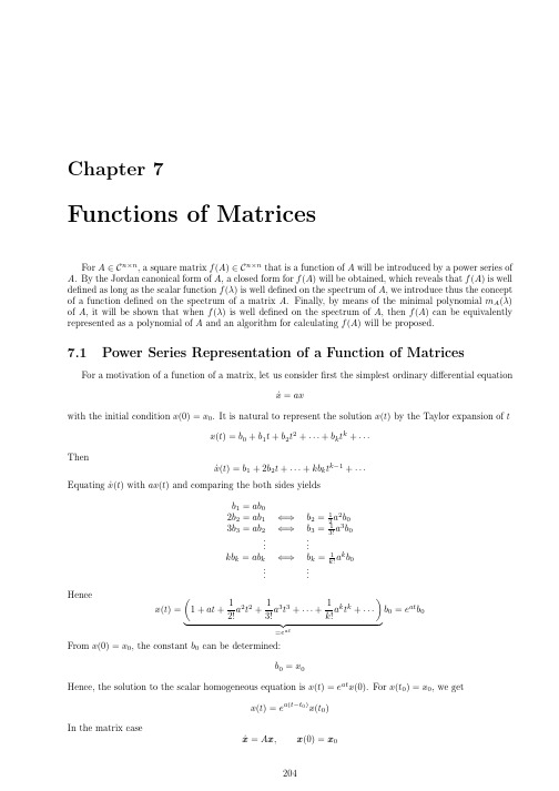
北京理工大学线性代数讲义第七章
x ˙ = ax
For a motivation of a function of a matrix, let us consider first the simplest ordinary differential equation
sin λ = cos λ = (1 + λ)−1 ln(1 + λ) we have = =
1 1 2 A + · · · + An + · · · ρ(A) < ∞ 2! n! 1 3 1 5 1 A2n+1 + · · · ρ(A) < ∞ sin A = A − A + A − · · · + (−1)n 3! 5! (2n + 1)! 1 1 1 cos A = E − A2 + A4 − · · · + (−1)n A2n + · · · ρ(A) < ∞ 2! 4! (2n)! eA = E+A+ (E + A)−1 ln(E + A) = E − A + A2 − A3 + · · · + (−1)n An + · · · ρ(A) < 1 1 1 1 = E − A2 + A3 − · · · + (−1)n+1 An + · · · ρ(A) < 1 2 3 n!
2 b2 = 1 2 A b0 1 3 b3 = 3! A b0 . . .
bk = . . .
1 k k! A b0
1 2 2 1 1 A t + A3 t3 + · · · + Ak tk + · · · 2! 3! k!
A PTAS for the Multiple Knapsack Problem

A PTAS for the Multiple Knapsack ProblemChandra Chekuri Sanjeev KhannaAbstractThe Multiple Knapsack problem(MKP)is a natural and well knowngeneralization of the single knapsack problem and is defined asfollows.We are given a set of items and bins(knapsacks)suchthat each item has a profit and a size,and each bin hasa capacity.The goal is tofind a subset of items of maximumprofit such that they have a feasible packing in the bins.MKP is aspecial case of the Generalized Assignment problem(GAP)wherethe profit and the size of an item can vary based on the specific binthat it is assigned to.GAP is APX-hard and a-approximation for itis implicit in the work of Shmoys and Tardos[26],and thus far,thiswas also the best known approximation for MKP.The main resultof this paper is a polynomial time approximation scheme for MKP.Apart from its inherent theoretical interest as a common gen-eralization of the well-studied knapsack and bin packing problems,it appears to be the strongest special case of GAP that is not APX-hard.We substantiate this by showing that slight generalizationsof MKP are APX-hard.Thus our results help demarcate the bound-ary at which instances of GAP become APX-hard.An interestingand novel aspect of our approach is an approximation preservingreduction from an arbitrary instance of MKP to an instance withdistinct sizes and profits.1IntroductionWe study the following natural generalization of the classicalknapsack problem:Multiple Knapsack Problem(MKP)I NSTANCE:A pair where is a set of bins(knapsacks)and is a set of items.Each bin hasa capacity,and each item has a size and a profit.O BJECTIVE:Find a subset of maximum profit suchthat has a feasible packing in.The decision version of MKP is a generalization of thedecision versions of both the knapsack and bin packingproblems and is strongly NP-Complete.Moreover,it isan important special case of the generalized assignmentproblem where both the size and the profit of an item area function of the bin:1GAP has also been defined in the literature as a(closely related)minimization problem(see[26]).In this paper,following[24],we referto the maximization version of the problem as GAP and refer to theminimization version as Min GAP.item sizes and profits as well as bin capacities may take anyarbitrary values.Establishing a PTAS would show a very fine separation between cases that are APX-hard and thosethat have a PTAS.Until now,the best known approximationratio for MKP was a factor of derived from the approxima-tion for GAP.Our main result:In this paper we resolve the approxima-bility of MKP by obtaining a PTAS for it.It can be easilyshown via a reduction from the Partition problem that MKPdoes not admit a FPTAS even if.A special case of MKP is when all bin capacities are equal.It is relativelystraightforward to obtain a PTAS for this case using ideas from approximation schemes for knapsack and bin packing[11,3,15].However the general case with different bincapacities is a non-trivial and challenging problem.Our paper contains two new technical ideas.Ourfirst idea con-cerns the set of items to be packed in a knapsack instance.We show how to guess,in polynomial time,almost all the items that are to be packed in a given knapsack instance.Inother words we can identify an item set that has a feasible packing and profit at least OPT.This is in contrastto earlier schemes for variants of knapsack[11,1,5]whereonly the most profitable items are guessed.An easy corollary of our strategy is a PTAS for the identical bincapacity case,the details of which we point out later.Thestrengthened guessing plays a crucial role in the general case in the following way.As a byproduct of our guessingscheme we show how to round the sizes of items to at most distinct sizes.An immediate consequence of this is a quasi-polynomial time algorithm to pack items intobins using standard dynamic programming.Our second set of ideas shows that we can exploit the restricted sizesto pack,in polynomial time,a subset of the item set thathas at least a fraction of the profit.Approximation schemes for number problems are usually based on rounding instances to have afixed number of distinct values.In contrast,MKP appears to require a logarithmic number of values.We believe that our ideas to handle logarithmic number of distinct values willfind other applications.Figure 1summarizes the approximability of various restrictions of GAP.Related work:MKP is closely related to knapsack,bin packing,and GAP.A very efficient FPTAS exists for the knapsack problem;Lawler[17],based on ideas from[11], achieves a running time of for a approximation.An asymptotic FPTAS is known for bin packing[3,15].Recently Kellerer[16]has independently developed a PTAS for the special case of the MKP where all bins have identical capacity.As mentioned earlier, this case is much simpler than the general case and falls out as a consequence of ourfirst idea.The generalized assignment problem,as we phrased it,seeks to maximize profit of items packed.This is natural when viewed as a knapsack problem(see[24]).The minimization version of the problem,referred to as Min GAP and also as the cost assignment problem,seeks to assign all the items while minimizing the sum of the costs of assigning items to bins. In this version,item incurs a cost if assigned to bin instead of a obtaining a profit.Since the feasibility of assigning all items is itself an NP-Complete problem we need to relax the bin capacity constraints.Anbi-criteria approximation algorithm for Min GAP is one that gives a solution with cost at most and with bin capacities violated by a factor of at most where is the cost of an optimal solution that does not violate any capacity constraints.Work of Lin and Vitter[20]yields a approximation for Min GAP.Shmoys and Tardos[26],building on the work of Lenstra,Shmoys, and Tardos[19],give an improved approximation. Implicit in this approximation is also a-approximation for the profit maximization version which we sketch later. Lenstra et al.[19]also show that it is NP-hard to obtain a ratio for any.The hardness relies on a NP-Completeness reduction from3-Dimensional Matching. Our APX-hardness for the maximization version,mentioned earlier,is based on a similar reduction but instead relies on APX-hardness of the optimization version of3-Dimensional matching[14].MKP is also related to two variants of variable size bin packing.In thefirst variant we are given a set of items and set of bin capacities.The objective is tofind a feasible packing of items using bins with capacities restricted to be from so as to minimize the sum of the capacities of the bins used.A PTAS for this problem was provided by Murgolo [25].The second variant is based on a connection to multi-processor scheduling on uniformly related machines[18]. The objective is to assign a set of independent jobs with given processing times to machines with different speeds to minimize the makespan of the schedule.Hochbaum and Shymoys[8]gave a PTAS for this problem using a dual based approach where they convert the scheduling problem into the following bin packing problem.Given items of different sizes and bins of different capacities,find a packing of all the items into the bins such that maximum violation of the capacity of any bin is minimized. Bi-criteria approximations,where both capacity and profit can be approximated simultaneously,have been studied for several problems(Min GAP being an example mentioned above)and it is usually the case that relaxing both makes the task of approximation somewhat easier.In particular, relaxing the capacity constraints allows rounding of item sizes into a small number of distinct size values.In MKP we are neither allowed to exceed the capacity constraints nor the number of bins.This makes the problem harder and our result interesting.Knapsack GAPMultiple identical capacity binsNo FPTAS even with 2 binsItem size varies with binsvary with bins.Both size and profitMultiple non-identical capacity binsPTAS (special case of Theorem 2.1)2-approximable (Proposition 3.2, [26])if all sizes are identical (Proposition 3.1)However, it is polynomial time solvable only 2 distinct profits (Theorem 3.2)MKPPTAS (Theorem 2.1)(Theorem 3.1)APX-hard even when each item takes Item profit varies with binsFPTAS[10,15]sizes and all profits are identical.each item takes only 2 distinct APX-hard even whenFigure 1:Complexity of Various Restrictions of GAPOrganization:Section 2describes our PTAS for MKP.In Section 3,we show that GAP is APX-hard on very restricted classes of instances.We also indicate here a -approximation for GAP.In Section 4,we discuss a natural greedy algorithmfor MKP and show that it gives a-approximation even when item sizes vary with bins.2A PTAS for the Multiple Knapsack Problem We denote by OPT the value of an optimal solution to thegiven instance.Given a setof items,we use to denote .The set of integers is denoted by .Our problem is related to both the knapsack problem and the bin packing problem and some ideas used in approximation schemes for those problems will be useful to us.Our approximation scheme conceptually has the following two steps.1.G UESSING I TEMS :Identify a set of itemssuch that OPT and has a feasible packing in .2.P ACKING I TEMS :Given a setof items that has a feasible packing in ,find a feasible packing for a set such that .The overall scheme is more involved since there is interaction between the two steps.The guessed items have some additional properties that are exploited in the packing step.We observe that both of the above steps require new ideas.For the single knapsack problem no previous algorithm identifies the full set of items to pack.Moreover testing the feasibility of packing a given set of items is trivial.However in MKP the packing step is itself quite complex and it seems necessary to decompose the problem as we did.Before we proceed with the details we show how the first step of guessing the items immediately gives a PTAS for the identical bin capacity case.2.1MKP with Identical Bin CapacitiesSuppose we can guess an item set as in our first step above.We show that the packing step is very simple if bin capacities are identical.There are two cases to consider depending on whether ,the number of bins,is less than or not.In the former case the number of bins can be treated as a constant and a PTAS for this case exists even for instances of GAP (implicit in earlier work [5]).Now suppose .We use the any of the known PTASs for bin packing andpack all the guessed items using at mostbins.We find a feasible solution by simply picking the largest profit bins and discarding the rest along with their items.Here weuse the fact that and that the bins are identical.It is easily seen that we get aapproximation.We note that a different PTAS,without using our guessing step,can be obtained for this case by directly adapting the ideas used in approximation schemes for bin packing.The trick of using extra bins does not have a simple analogue when bin capacities are different and we need more ideas.2.2Guessing ItemsConsider the case when items have the same profit(assume it is).Thus the objective is to pack as many items as possible.For this case it is easily seen that OPT is an integer in.Further,given a guess for OPT,we can always pick the smallest(in size)OPT items to pack.Therefore there are only a polynomial number of guesses for the set of items to pack. This idea does not have a direct extension to non-uniform profits.However the useful insight is that when profits are identical we can pick the items in order of their sizes.In the rest of the paper we assume,for simplicity of notation,that and are integers.For the general case thefirst step in guessing items involves massaging the given instance into a more structured one that has few distinct profits.This is accomplished as follows.1.Guess a value such that OPT OPTand discard all items where.2.Scale all profits by such that they are in the range.3.Round down the profits of items to the nearest power of.Thefirst two steps are similar to those in the FPTAS for the single knapsack problem.It is easily seen that at most an fraction of the optimal profit is lost by our transformation.Summarizing:L EMMA2.1.Given an instance with items and a value such that OPT OPT we can obtain in polynomial time another instancesuch that.For every,for some.OPTitems.We discard the items in and for each we increase the size of every item in to the size of the smallest item in.Since is ordered by size no item in is larger than the smallest item in for each.It is easy to see that if has a feasible packing then the modified instance also has a feasible packing.We discard at most an fraction of the profit and the modified sizes have at most distinct values.Applying this to each profit class we obtain an instance with distinct size values.L EMMA2.3.Given an instance with items we can obtain in polynomial time instances such thatFor,and has items only from distinct profit values.For,and has items only from distinct size values.There exists an index such that has a feasible packing in and OPT.We will assume for the next section that we have guessed the correct set of items and that they are partitioned into sets with each set containing items of the same size.We denote by the items of the th size value and by the quantity.2.3Packing ItemsFrom Lemma2.3we obtain a restricted set of instances in terms of item profits and sizes.We also need some structure in the bins and we start by describing the necessary transformations.2.3.1Structuring the BinsAssume without loss of generality that the smallest bin capacity is.We order the bins in increasing order of their capacity and partition them into blocks such that block consists of all bins with.Let denote the number of bins in block.D EFINITION2.1.(Small rge Blocks)A block of bins is called a small bin block if;it is called large otherwise.Let be the set of indices such that is small.Define to be the set of largest indices in the set.Let and be the set of all bins in the blocks specified by the index sets and respectively.The following lemma makes use of the property of geometrically increasing bin capacities.L EMMA2.4.Let be a set of items that can be packed in the bins.There exists a set such that can be packed into the bins,and.Proof.Fix some packing of in the bins.Consider the largest bins in.One of these bins has a profit less than.Without loss of generality assume its capacity is.We will remove the items packed in this bin and use it to pack items from smaller bins.Let be the block containing this bin.Bins in block where andhave a capacity less than.It is easy to verify that the total capacity of bins in small bin blocks with indices less than equal to is at most.Since each of the first bins could be in different blocks the upper bound of blocks follows.Therefore we can retain the small bin blocks of large capacity and discard the rest.Therefore we as-sume that the given instance is modified to satisfy.Then it follows that. When the number of bins isfixed a PTAS is known(implicit in earlier work)even for the GAP.We will use ideas from that algorithm.For large bin blocks the advantage is that we can exceed the number of bins used by an fraction,as we shall see below.The main task is to integrate the allocation and packing of items between the different sets of bins.For the rest of the section we assume that we have a set of items that have a feasible packing and we will implicitly refer to somefixed feasible packing as the optimal solution.2.3.2Packing Profitable Items into Small Bin Blocks We guess here for each bin in,the most profitable items that are packed in it in the optimal solution.Therefore the number of guesses needed is.2.3.3Packing Large Items into Large Bin BlocksThe second step is to select items and pack them in large bin blocks.We say that an item is packed as a large item if its size is at least times the capacity of the bin in which it is packed.Since the capacities of the blocks are increasing geometrically,an item can be packed as large in at mostCombining for all sizes results in guesses over all.Here is where we take advantage of the fact that our items come from only different size classes.Suppose we have correctly assigned all large items to their respective bin blocks.We describe now a procedure for finding a feasible packing of these items.Here we ignore the potential interaction between items that are packed as large and those packed as small.We will show later that we can do so with only a slight loss in the approximation factor.We can focus on a specific block since the large items are now partitioned between the blocks.The abstract problem we have is the following.Given a collection of bins with capacities in the range,and a set of items with sizes in the range,decide if there is a feasible packing for them.It is easily seen that this problem is NP-hard.We obtain a relaxation by allowing use of extra bins to pack the items.However,we restrict the capacity of the extra bins to be.The following algorithm decides that either the given instance is infeasible or gives a packing with at most an additional bins of capacity.Let be the set of items of size greater than.Order items of in non-decreasing sizes and pack each item into the smallest bin available that can accommodate it.Disregard all the bins used up in the previous step since no other large item canfit into them.To pack the remaining items use a PTAS for bin pack-ing,potentially using an extra bins of capacity.We omit the full details of the algorithm but summarize the result in the following lemma.L EMMA2.5.Given bins of capacities in the range and items of sizes in the range,there is an algorithm that runs in time,and provided the items have a feasible packing in the given bins,returns a feasible packing using at most extra bins of capacity.We eliminate the extra bins later by picking the most profitable among them and discarding the items packed in the rest.The restriction on the size and number of extra bins is motivated by the elimination procedure.In order to use extra bins the quantity needs to be at least.This is the reason to distinguish between small and large bin blocks.For a large bin block let be the extra bins used in packing the large items.We note that.2.3.4Packing the Remaining ItemsThe third and last step of the algorithm is to pack the remaining items which we denote by.At this stage we have a packing of the most profitable items in each of the bins in(bins in small bin blocks)and a feasiblepacking of the large items in the rest of the bins(including the extra bins).For each bin let denote the set of items already packed into in thefirst two steps.The itemset is packed via an LP approach.In particular we use the generalized assignment formulation with the following constraints.1.Each remaining item must be assigned to some bin.2.An item can can be assigned to a bin in a large binblock only if.In other wordsshould be small for all bins in.3.An item can be assigned to a bin in a small binblock only ifassigned to the bins satisfy the constraints specified by, that is if.The integral solution to the LP also defines an allocation of items to each block.Let be the total profit associated with all items assigned to bins in block.Then clearly,.We however have an infeasible solution.Extra bins are used for large bin blocks and bin capacities are violated in the rounded solution.We modify this solution to create a feasible solution such that in each block we obtain a profit of at least .Large Bin Blocks:Let be a large bin block and without loss of generality assume that bin capacities in are in the range.By constraint2on the assignment,the size of any violating item in is less than and there are at most of them.For all we conclude that at most extra bins of capacity each are sufficient to pack all the violating items of.Recall that we may have used extra bins in packing the large items as well.Thus the total number of extra bins of capacity,denoted by,is at most .Thus all items assigned to bins in have a feasible integral assignment in the set.Now clearly the most profitable bins in the collection must have a total associated profit of at least.Moreover,it is easy to verify that all the items in these bins can be packed in the bins of itself.Small Bin Blocks:Consider now a small bin block. By constraint3on the assignment,we know that the profit associated with the violating item in any bin of is at most.For each element of we have an item in and similarly for and for.We also have an additional items whereand for any additional item and a bin. Fix a positive constant.For an item and bin we set if and otherwise.The profits of items and are set similarly.The sizes of items, and are all set to1each.It is now easy to verify that if instance has a matching of size,there exists a solution to of value.Otherwise,every solution to has value at most.As above,the APX-hardness now follows from the fact that.Notice that Theorem3.2is not a symmetric analogue of Theorem3.1.In particular,we use items of two different sizes in Theorem3.2.This is necessary as the special case of GAP where all item sizes are identical across the bins (but the profits can vary from bin to bin),is equivalent to minimum cost bipartite matching.P ROPOSITION3.1.There is a polynomial time algorithm to solve GAP instances where all items have identical sizes across the bins.3.2A-approximation for GAPShmoys and Tardos[26]give a bi-criteria approxima-tion for Min GAP.A paraphrased statement of their precise result is as follows.T HEOREM3.3.(S HMOYS AND T ARDOS[26])Given a feasible instance for the cost assignment problem,there is a polynomial time algorithm that produces an integral assignment such thatcost of solution is no more than OPT,each item assigned to a bin satisfies, andif a bin’s capacity is violated then there exists a single item that is assigned to the bin whose removal ensures feasibility.We now indicate how the above theorem implies a-approximation for GAP.The idea is to simply convert the maximization problem to a minimization problem by turning profits into costs by setting whereis a large enough number to make all costs positive.To create a feasible instance we have an additional bin of capacity and for all items we set and(in other words).We then use the algorithm for cost assignment and obtain a solution with the guarantees provided in Theorem3.3.It is easily seen that the profit obtained by the assignment is at least the optimal profit.Nowwe show how to obtain a feasible solution of at least half the profit.Let be any bin whose capacity is violated by the assignment and let be the item guaranteed in Theorem3.3.If is at least half the profit of bin then we retain and leave out the rest of the items in.In the other casewe leave out.This results in a feasible solution of at least half the profit given by the LP solution.We get the following result:P ROPOSITION3.2.There is a-approximation for GAP.R EMARK3.1.The algorithm in[26]is based on rounding an LP relaxation.For MKP an optimal solution to the linear program can be easily constructed in time byfirst sorting items by their profit to size ratio and then greedily filling them in the bins.Rounding takes time. We also note that the integrality gap for the LP relaxation of GAP is a factor of even for instances of MKP with identical bin capacities.4A Greedy AlgorithmWe now analyse a natural greedy strategy:pack bins oneat a time,by applying the FPTAS for the single knapsack problem on the remaining items.Greedy(refers to this algorithm with parameterizing the error tolerance used in the knapsack FPTAS.C LAIM4.1.For instances of MKP with bins of identical capacity Greedy()gives aR EMARK4.1.Claim4.2is valid even if the item sizes(but not profits)are a function of the bins,an important specialcase of GAP that is already APX-hard.The running time of Greedy()is using the algorithm of Lawler[17]for the knapsack problem.Claim4.2has beenindependently observed in[2].A Tight Example:We show an instance on which Greedy’s performance is no better than.There are two items with sizes and and each has a profit of.There are two bins with capacities and each.Greedy packs the smaller item in the big bin and obtains a profit of while OPT.This also shows that ordering bins in non-increasing capacities does not help improve the performance of Greedy.5ConclusionsAn interesting aspect of our guessing strategy is that it is completely independent of the number of bins and their capacities.This might prove to be useful in other variants of the knapsack problem.One recent application is in obtaining a PTAS for the stochastic knapsack problem with Bernoulli variables[7].The Min GAP problem has a bi-criteria ap-proximation and it is NP-hard to obtain a-approximation.In contrast GAP has a-approximation but the known hardness of approximation is for a very small butfixed.Closing this gap is an interesting open problem.Another interesting problem is to obtain a PTAS for MKP with an improved running time.Though an FPTAS is ruled out even for the case of two identical bins,a PTAS with a running time of the form poly might be achievable.The identical bin capacities case might be more tractable than the general case.Extending our ideas to achieve the above mentioned running time appears to be non-trivial.References[1] A.K.Chandra,D.S.Hirschberg,and C.K.Wong.Approx-imate algorithms for some generalized knapsack problems.Theoretical Computer Science,3(3):293–304,Dec1976. [2]M.W.Dawande,J.R.Kalagnanam,P.Keskinocak,R.Ravi,and F.S.Salman.Approximation algorithms for the multiple knapsack problem with assignment restrictions.Technical Report,RC21331,IBM T.J.Watson Research Center,1998.[3]W.Fernandez de la Vega and G.S.Lueker.Bin packing canbe solved within in linear binatorica,1:349–355,1981.[4] C.E.Ferreira, A.Martin,and R.Weismantel.Solvingmultiple knapsack problems by cutting planes.SIAM Journal on Optimization,6(3):858–77,1996.[5] A.M.Frieze and M.R.B.Clarke.Approximation algorithmsfor the-dimensional-knapsack problem:worst-case and probabilistic analyses.European Journal of Operational Research,15(1):100–9,1984.[6]M.R.Garey and puters and Intractabil-ity:A Guide to the Theory of NP-Completeness.Freeman, 1979.[7] A.Goel and P.Indyk.Stochastic load balancing and relatedproblems.In Proceedings of the40th Annual Symposium on Foundations of Computer Science,pages579–86,1999. [8] D.S.Hochbaum and D.B.Shmoys.A polynomial approxi-mation scheme for scheduling on uniform processors:using the dual approximation approach.SIAM Journal on Comput-ing,17:539–551,1988.[9]M.S.Hung and J.C.Fisk.An algorithm for0-1multipleknapsack problems.Naval Research Logistical Quarterly, 24:571–579,1978.[10]M.S.Hung and J.C.Fisk.A heuristic routine for solvinglarge loading problems.Naval Research Logistical Quar-terly,26(4):643–50,1979.[11]O.H.Ibarra and C.E.Kim.Fast approximation algorithmsfor the knapsack and sum of subset problems.Journal of the ACM,22(4):463–8,1975.[12]G.Ingargiola and J.F.Korsh.An algorithm for the solution of0-1loading problems.Operations Research,23(6):110–119, 1975.[13]J.R.Kalagnanam,M.W.Dawande,M.Trubmo,and H.S.Lee.Inventory problems in steel industry.Technical Report, RC21171,IBM T.J.Watson Research Center,1998.[14]V.Kann.Maximum bounded-dimensional matching ismax rmation Processing Letters,37:27–35,1991.[15]N.Karmarkar and R.Karp.An efficient approximationscheme for the one-dimensional bin-packing problem.In Proceedings of the23rd Annual Symposium on Foundations of Computer Science,pages312–320,1982.[16]H.Kellerer.A Polynomial Time Approximation Schemefor the Multiple Knapsack Problem.In Proceedings of APPROX’99,Springer.[17] wler.Fast approximation algorithms for knapsackproblems.Mathematics of Operations Research,4(4):339–56,1979.[18] wler,J.K.Lenstra,A.H.G.Rinnooy Kan,andD.B.Shmoys.Sequencing and scheduling:algorithms andcomplexity.In S.C.Graves et al.,editor,Handbooks in OR &MS,volume4,pages445–522.Elsevier Science Publishers, 1993.[19]J.K.Lenstra,D.B.Shmoys,and E.Tardos.Approximationalgorithms for scheduling unrelated parallel machines.Math-ematical Programming,46:259–271,1990.Preliminary ver-sion appeared in Proceedings of the28th Annual IEEE Sym-posium on Foundations of Computer Science,217–24,1987.[20]J.Lin and J.S.Vitter.-Approximations with minimumpacking constraint.In Proceedings of the24th Annual ACM Symposium on Theory of Computing,771–782,1992. [21]S.Martello and P.Toth.Solution of the zero-one multipleknapsack problem.European J.of Operations Research, 4:322–329,1980.。
A Sequential Algorithm for Generating Random Graphs

Mohsen Bd Amin Saberi1
arXiv:cs/0702124v4 [] 16 Jun 2007
Stanford University {bayati,saberi}@ 2 Yonsei University jehkim@yonsei.ac.kr
(FPRAS) for generating random graphs; this we can do in almost linear time. An FPRAS provides an arbitrary close approximaiton in time that depends only polynomially on the input size and the desired error. (For precise definitions of this, see Section 2.) Recently, sequential importance sampling (SIS) has been suggested as a more suitable approach for designing fast algorithms for this and other similar problems [18, 13, 35, 6]. Chen et al. [18] used the SIS method to generate bipartite graphs with a given degree sequence. Later Blitzstein and Diaconis [13] used a similar approach to generate general graphs. Almost all existing work on SIS method are justified only through simulations and for some special cases counter examples have been proposed [11]. However the simplicity of these algorithms and their great performance in several instances, suggest further study of the SIS method is necessary. Our Result. Let d1 , . . . , dn be non-negative integers given for the degree sequence n and let i=1 di = 2m. Our algorithm is as follows: start with an empty graph and sequentially add edges between pairs of non-adjacent vertices. In every step of the procedure, the probability that an edge is added between two distinct ˆj (1 − di dj /4m) where d ˆi and d ˆj denote ˆi d vertices i and j is proportional to d the remaining degrees of vertices i and j . We will show that our algorithm produces an asymptotically uniform sample with running time of O(m dmax ) when maximum degree is of O(m1/4−τ ) and τ is any positive constant. Then we use a simple SIS method to obtain an FPRAS for any ep, δ > 0 with running time O(m dmax ǫ−2 log(1/δ )) for generating graphs with dmax = O(m1/4−τ ). Moreover, we show that for d = O(n1/2−τ ), our algorithm can generate an asymptotically uniform d-regular graph. Our results are improving the bounds of Kim and Vu [34] and Steger and Wormald [45] for regular graphs. Related Work. McKay and Wormald [37, 39] give asymptotic estimates for number of graphs within the range dmax = O(m1/3−τ ). But, the error terms in their estimates are larger than what is needed to apply Jerrum, Valiant and Vazirani’s [25] reduction to achieve asymptotic sampling. Jerrum and Sinclair [26] however, use a random walk on the self-reducibility tree and give an FPRAS for sampling graphs with maximum degree of o(m1/4 ). The running time of their algorithm is O(m3 n2 ǫ−2 log(1/δ )) [44]. A different random walk studied by [27, 28, 10] gives an FPRAS for random generation for all degree sequences for bipartite graphs and almost all degree sequences for general graphs. However the running time of these algorithms is at least O(n4 m3 dmax log5 (n2 /ǫ)ǫ−2 log(1/δ )). For the weaker problem of generating asymptotically uniform samples (not an FPRAS) the best algorithm was given by McKay and Wormald’s switching technique on configuration model [38]. Their algorithm works for graphs 2 2 3 2 with d3 max =O(m / i di ) with average running i di ) and dmax = o(m + 2 2 2 4 time of O(m + ( i di ) ). This leads to O(n d ) average running time for dregular graphs with d = o(n1/3 ). Very recently and independently from our work, Blanchet [12] have used McKay’s estimate and SIS technique to obtain an FPRAS with running time O(m2 ) for sampling bipartite graphs with given
关于polyfit 函数使用介绍

关于polyfit 函数使用介绍文章来源:不详作者:佚名--------------------------------------------------------------------------------该文章讲述了关于polyfit 函数使用介绍.polyfit函数的使用MATLAB软件提供了基本的曲线拟合函数的命令.多项式函数拟合:P=polyfit(x,y,n)其中n表示多项式的最高阶数,x,y为将要拟合的数据,它是用数组的方式输入.输出参数P为拟合多项式P(1)*X^N + P(2)*X^(N-1) +...+ P(N)*X + P(N+1).的系数多项式在x处的值y可用下面程序计算.y=polyval(P,x,m)线性:m=1, 二次:m=2, …polyfit的输出是一个多项式系数的行向量。
为了计算在xi数据点的多项式值,调用MATLAB 的函数polyval。
例:x=0:0.1:1;y=[-0.447 1.978 3.28 6.16 7.08 7.34 7.66 9.56 9.48 9.30 11.2];A=polyfit(x,y,2)Z=polyval(A,x);Plot(x,y,’r*’,x,z,’b’)polyfit不能保证你每次都能得到最优解,math的答案是使用数值计算。
个人认为,对于这种非线性的曲线,尽量不要使用ployfit, ployfit多项式抑合适合线性方程!!用polyfit()函数去拟合这么复杂的曲线不太合适,polyfit()函数对于数据遵循多项式分布是比较好的,一般来说,利用polyfit()函数拟合的阶数不要超过5阶。
如果是不需要得到拟合曲线的函数,只是把这些点利用一些光滑曲线连接,建议使用三次样条函数spline()进行插值即可。
帮助:POL YFIT Fit polynomial to data.P = POL YFIT(X,Y,N) finds the coefficients of a polynomial P(X) ofdegree N that fits the data Y best in a least-squares sense. P is arow vector of length N+1 containing the polynomial coefficients indescending powers, P(1)*X^N + P(2)*X^(N-1) +...+ P(N)*X + P(N+1).[P,S] = POL YFIT(X,Y,N) returns the polynomial coefficients P and astructure S for use with POL YV AL to obtain error estimates forpredictions. S contains fields for the triangular factor (R) from a QRdecomposition of the Vandermonde matrix of X, the degrees of freedom(df), and the norm of the residuals (normr). If the data Y are random,an estimate of the covariance matrix of P is (Rinv*Rinv')*normr^2/df,where Rinv is the inverse of R.[P,S,MU] = POL YFIT(X,Y,N) finds the coefficients of a polynomial inXHAT = (X-MU(1))/MU(2) where MU(1) = MEAN(X) and MU(2) = STD(X). Thiscentering and scaling transformation improves the numerical propertiesof both the polynomial and the fitting algorithm.Warning messages result if N is >= length(X), if X has repeated, ornearly repeated, points, or if X might need centering and scaling.Class support for inputs X,Y:float: double, singlepolyfit.m 在MATLAB安装目录下\toolbox\matlab\polyfunfunction [p,S,mu] = polyfit(x,y,n)%POLYFIT Fit polynomial to data.% P = POLYFIT(X,Y,N) finds the coefficients of a polynomial P(X) of% degree N that fits the data Y best in a least-squares sense. P is a% row vector of length N+1 containing the polynomial coefficients in% descending powers, P(1)*X^N + P(2)*X^(N-1) +...+ P(N)*X + P(N+1).%% [P,S] = POLYFIT(X,Y,N) returns the polynomial coefficients P and a% structure S for use with POLYVAL to obtain error estimates for% predictions. S contains fields for the triangular factor (R) from a QR% decomposition of the Vandermonde matrix of X, the degrees of freedom % (df), and the norm of the residuals (normr). If the data Y are random,% an estimate of the covariance matrix of P is (Rinv*Rinv')*normr^2/df,% where Rinv is the inverse of R.%% [P,S,MU] = POLYFIT(X,Y,N) finds the coefficients of a polynomial in% XHAT = (X-MU(1))/MU(2) where MU(1) = MEAN(X) and MU(2) = STD(X). This% centering and scaling transformation improves the numerical properties % of both the polynomial and the fitting algorithm.%% Warning messages result if N is >= length(X), if X has repeated, or% nearly repeated, points, or if X might need centering and scaling.%% Class support for inputs X,Y:% float: double, single%% See also POLY, POLYVAL, ROOTS.% Copyright 1984-2004 The MathWorks, Inc.% $Revision: 5.17.4.5 $ $Date: 2004/07/05 17:01:37 $% The regression problem is formulated in matrix format as:%% y = V*p or%% 3 2% y = [x x x 1] [p3% p2% p1% p0]%% where the vector p contains the coefficients to be found. For a% 7th order polynomial, matrix V would be:%% V = [x.^7 x.^6 x.^5 x.^4 x.^3 x.^2 x ones(size(x))];if ~isequal(size(x),size(y))error('MATLAB:polyfit:XYSizeMismatch',...'X and Y vectors must be the same size.')endx = x(:);y = y(:);if nargout > 2mu = [mean(x); std(x)];x = (x - mu(1))/mu(2);end% Construct Vandermonde matrix.V(:,n+1) = ones(length(x),1,class(x));for j = n:-1:1V(:,j) = x.*V(:,j+1);end% Solve least squares problem.[Q,R] = qr(V,0);ws = warning('off','all');p = R\(Q'*y); % Same as p = V\y;warning(ws);if size(R,2) > size(R,1)warning('MATLAB:polyfit:PolyNotUnique', ...'Polynomial is not unique; degree >= number of data points.')elseif condest(R) > 1.0e10if nargout > 2warning('MATLAB:polyfit:RepeatedPoints', ...'Polynomial is badly conditioned. Remove repeated data points.') elsewarning('MATLAB:polyfit:RepeatedPointsOrRescale', ...['Polynomial is badly conditioned. Remove repeated datapoints\n' ...' or try centering and scaling as described in HELP POLYFIT.'])endendr = y - V*p;p = p.'; % Polynomial coefficients are row vectors by convention.% S is a structure containing three elements: the triangular factor from a% QR decomposition of the Vandermonde matrix, the degrees of freedom and % the norm of the residuals.S.R = R;S.df = length(y) - (n+1);S.normr = norm(r);。
关于polyfit 函数使用介绍
关于polyfit 函数使用介绍文章来源:不详作者:佚名--------------------------------------------------------------------------------该文章讲述了关于polyfit 函数使用介绍.polyfit函数的使用MATLAB软件提供了基本的曲线拟合函数的命令.多项式函数拟合:P=polyfit(x,y,n)其中n表示多项式的最高阶数,x,y为将要拟合的数据,它是用数组的方式输入.输出参数P为拟合多项式P(1)*X^N + P(2)*X^(N-1) +...+ P(N)*X + P(N+1).的系数多项式在x处的值y可用下面程序计算.y=polyval(P,x,m)线性:m=1, 二次:m=2, …polyfit的输出是一个多项式系数的行向量。
为了计算在xi数据点的多项式值,调用MATLAB 的函数polyval。
例:x=0:0.1:1;y=[-0.447 1.978 3.28 6.16 7.08 7.34 7.66 9.56 9.48 9.30 11.2];A=polyfit(x,y,2)Z=polyval(A,x);Plot(x,y,’r*’,x,z,’b’)polyfit不能保证你每次都能得到最优解,math的答案是使用数值计算。
个人认为,对于这种非线性的曲线,尽量不要使用ployfit, ployfit多项式抑合适合线性方程!!用polyfit()函数去拟合这么复杂的曲线不太合适,polyfit()函数对于数据遵循多项式分布是比较好的,一般来说,利用polyfit()函数拟合的阶数不要超过5阶。
如果是不需要得到拟合曲线的函数,只是把这些点利用一些光滑曲线连接,建议使用三次样条函数spline()进行插值即可。
帮助:POL YFIT Fit polynomial to data.P = POL YFIT(X,Y,N) finds the coefficients of a polynomial P(X) ofdegree N that fits the data Y best in a least-squares sense. P is arow vector of length N+1 containing the polynomial coefficients indescending powers, P(1)*X^N + P(2)*X^(N-1) +...+ P(N)*X + P(N+1).[P,S] = POL YFIT(X,Y,N) returns the polynomial coefficients P and astructure S for use with POL YV AL to obtain error estimates forpredictions. S contains fields for the triangular factor (R) from a QRdecomposition of the Vandermonde matrix of X, the degrees of freedom(df), and the norm of the residuals (normr). If the data Y are random,an estimate of the covariance matrix of P is (Rinv*Rinv')*normr^2/df,where Rinv is the inverse of R.[P,S,MU] = POL YFIT(X,Y,N) finds the coefficients of a polynomial inXHAT = (X-MU(1))/MU(2) where MU(1) = MEAN(X) and MU(2) = STD(X). Thiscentering and scaling transformation improves the numerical propertiesof both the polynomial and the fitting algorithm.Warning messages result if N is >= length(X), if X has repeated, ornearly repeated, points, or if X might need centering and scaling.Class support for inputs X,Y:float: double, singlepolyfit.m 在MATLAB安装目录下\toolbox\matlab\polyfunfunction [p,S,mu] = polyfit(x,y,n)%POLYFIT Fit polynomial to data.% P = POLYFIT(X,Y,N) finds the coefficients of a polynomial P(X) of% degree N that fits the data Y best in a least-squares sense. P is a% row vector of length N+1 containing the polynomial coefficients in% descending powers, P(1)*X^N + P(2)*X^(N-1) +...+ P(N)*X + P(N+1).%% [P,S] = POLYFIT(X,Y,N) returns the polynomial coefficients P and a% structure S for use with POLYVAL to obtain error estimates for% predictions. S contains fields for the triangular factor (R) from a QR% decomposition of the Vandermonde matrix of X, the degrees of freedom % (df), and the norm of the residuals (normr). If the data Y are random,% an estimate of the covariance matrix of P is (Rinv*Rinv')*normr^2/df,% where Rinv is the inverse of R.%% [P,S,MU] = POLYFIT(X,Y,N) finds the coefficients of a polynomial in% XHAT = (X-MU(1))/MU(2) where MU(1) = MEAN(X) and MU(2) = STD(X). This% centering and scaling transformation improves the numerical properties % of both the polynomial and the fitting algorithm.%% Warning messages result if N is >= length(X), if X has repeated, or% nearly repeated, points, or if X might need centering and scaling.%% Class support for inputs X,Y:% float: double, single%% See also POLY, POLYVAL, ROOTS.% Copyright 1984-2004 The MathWorks, Inc.% $Revision: 5.17.4.5 $ $Date: 2004/07/05 17:01:37 $% The regression problem is formulated in matrix format as:%% y = V*p or%% 3 2% y = [x x x 1] [p3% p2% p1% p0]%% where the vector p contains the coefficients to be found. For a% 7th order polynomial, matrix V would be:%% V = [x.^7 x.^6 x.^5 x.^4 x.^3 x.^2 x ones(size(x))];if ~isequal(size(x),size(y))error('MATLAB:polyfit:XYSizeMismatch',...'X and Y vectors must be the same size.')endx = x(:);y = y(:);if nargout > 2mu = [mean(x); std(x)];x = (x - mu(1))/mu(2);end% Construct Vandermonde matrix.V(:,n+1) = ones(length(x),1,class(x));for j = n:-1:1V(:,j) = x.*V(:,j+1);end% Solve least squares problem.[Q,R] = qr(V,0);ws = warning('off','all');p = R\(Q'*y); % Same as p = V\y;warning(ws);if size(R,2) > size(R,1)warning('MATLAB:polyfit:PolyNotUnique', ...'Polynomial is not unique; degree >= number of data points.')elseif condest(R) > 1.0e10if nargout > 2warning('MATLAB:polyfit:RepeatedPoints', ...'Polynomial is badly conditioned. Remove repeated data points.') elsewarning('MATLAB:polyfit:RepeatedPointsOrRescale', ...['Polynomial is badly conditioned. Remove repeated datapoints\n' ...' or try centering and scaling as described in HELP POLYFIT.'])endendr = y - V*p;p = p.'; % Polynomial coefficients are row vectors by convention.% S is a structure containing three elements: the triangular factor from a% QR decomposition of the Vandermonde matrix, the degrees of freedom and % the norm of the residuals.S.R = R;S.df = length(y) - (n+1);S.normr = norm(r);。
高阶滑模控制理论综述
第39卷第12期2022年12月控制理论与应用Control Theory&ApplicationsV ol.39No.12Dec.2022高阶滑模控制理论综述刘陆1,2,丁世宏1†,李世华2(1.江苏大学电气信息工程学院,江苏镇江212013;2.东南大学复杂工程系统测量与控制教育部重点实验室,江苏南京210096)摘要:滑模控制方法因其结构简单且对系统不确定及外部扰动具有良好的鲁棒性受到人们的广泛关注.因此,目前正处于飞速发展阶段.首先,本文回顾了滑模控制理论的起源,简单介绍了传统一阶滑模控制方法的发展;其次,列举了几种常用的二阶滑模控制方法,并介绍了其工作原理;接着,总结了高阶滑模控制理论的研究现状,主要包括齐次性算法和继电–多项式算法的研究成果;最后,结合高阶滑模控制方法中需要克服的问题,讨论了未来可能的研究方向.关键词:高阶滑模;齐次算法;继电–多项式算法;智能滑模;Lyapunov方法引用格式:刘陆,丁世宏,李世华.高阶滑模控制理论综述.控制理论与应用,2022,39(12):2193–2201DOI:10.7641/CTA.2022.10804A survey for high-order sliding mode control theoryLIU Lu1,2,DING Shi-hong1†,LI Shi-hua2(1.School of Electrical and Information Engineering,Jiangsu University,Zhenjiang Jiangsu212013,China;2.Key Laboratory of Measurement and Control of Complex Systems of Engineering,Ministry of Education,Southeast University,Nanjing Jiangsu210096,China)Abstract:The sliding mode control method has been paid much attention due to its simple structure and good robustness to system uncertainty and external disturbance.Therefore,it is in a stage of rapid development.Firstly,the survey reviews the origin of sliding mode control theory and briefly introduces the development of traditionalfirst-order sliding mode con-trol method.Secondly,we list several commonly used second-order sliding mode control methods,and then introduce their working principles.Next,the research status of high-order sliding mode control theory is summarized,mainly including the research results of the homogeneous algorithm and the relay-polynomial algorithm.Finally,combining with the problems that need to be overcome,the future outlook of high-order sliding mode control method is discussed.Key words:high order sliding mode;homogeneous algorithm;relay-polynomial algorithm;intelligent sliding mode; Lyapunov methodCitation:LIU Lu,DING Shihong,LI Shihua.A survey for high-order sliding mode control theory.Control Theory& Applications,2022,39(12):2193–22011引言滑模控制系统是一类特殊的变结构系统.早在20世纪50年代,前苏联工程师就已将变结构思想应用于实际系统,并且取得了良好的控制效果.后来,控制论专家Emelyanov,Utkin等学者对该控制思想产生了浓厚的兴趣,并从数学的角度对其进行了刻画和解释,首次提出了滑模控制理论这一概念[1–2].滑模控制的本质是使在规定的开关流形(滑模面)附近,受控状态轨迹的速度矢量总是指向开关流形.这种运动形式是通过施加破坏性(非连续)控制行为来诱导产生的,一般以开关控制策略的形式出现.通过上述控制作用,从空间任意一点出发的状态轨迹都能够在有限时间内到达滑模面(到达阶段),并沿着滑模面运动至平衡点(滑动模态阶段).值得一提的是,只有当系统状态始终满足滑模动力学时,理想的滑动模态才存在.通常来说,需要一个无限切换的开关方程才能确保滑动模收稿日期:2021−08−26;录用日期:2022−02−24.†通信作者.E-mail:***********.cn;Tel.:+86511-88787773.本文责任编委:孙健.国家自然科学基金项目(62103170,61973142),江苏省自然科学基金项目(BK20210745),江苏高校优势学科建设工程,东南大学复杂工程系统测量与控制教育部重点实验室开放课题项目(MCCSE2021A03)资助.Supported by the National Natural Science Foundation of China(62103170,61973142),the Natural Science Foundation of Jiangsu Province (BK20210745),the PAPD of Jiangsu Higher Education Institutions and the Open Project Fund of Key Laboratory of Measurement and Control of Complex Systems of Engineering,Ministry of Education,Southeast University(MCCSE2021A03).2194控制理论与应用第39卷态存在.得益于开关方程的非连续特性,滑模控制方法在应对参数摄动、未建模动态以及外部扰动等不确定性时具有强鲁棒性的特点.因而,自滑模控制理论成立以来,学者们对其进行了大量的理论与应用研究,文献[3–4]介绍了滑模控制理论形成初期的不同发展阶段及发展趋势,为滑模控制方法早起的发展提供了方向指导.进入21世纪以来,随着计算机行业的飞速发展,利用计算机的在线学习能力完成控制作用逐渐走进人们的视野.为此,文献[5]着重介绍了基于软计算技术的滑模控制理论的发展过程,并展望了其未来的发展趋势.在过去的十年中,研究表明,通过事件触发抽样取代时间抽样,可以提高抽样系统的整体性能.基于此,文献[6]介绍了不同的事件触发滑模控制策略的设计方法,并分析了它们的优缺点.另外,截至2021年10月25日,通过谷歌学术搜索关键词“sliding mode control ”,有192万条结果,这也从侧面反映出滑模控制理论是非线性控制领域中的一个新的研究热点.早期的滑模控制算法是基于线性滑模面构造的.例如,一般单输入–单输出线性系统可等价转化为可控标准型˙x =Ax +Bu ,这里x =[x 1···x n ]T ∈R n 为系统状态,u ∈R 为系统输入,矩阵A = 010···0001···0............000···1−a 1−a 2−a 3···−a n∈R n ×n ,B =[0···01]T ∈R n .基于线性滑模面s (x )=n ∑i =1c i x i ,c i >0,可设计常值切换的滑模控制器u =−β·sgn(s ),控制增益β是一个充分大的常数,以满足系统镇定的要求.进而,为了减弱扰动对闭环系统的影响,学者们提出了基于等效控制理论的滑模控制算法,该算法一般为u =u eq +u s 的形式,u eq 用来消除扰动对系统的影响,u s 为切换控制项.显而易见,由于用专门的等效控制项来处理系统扰动,所以其切换项增益可以很小,从而能够避免过大的抖振问题.但是,如前文所述,只有当系统处于滑动模态时,才对满足匹配条件的外界干扰、模型不确定性和未建模动态具有不变性,这说明,在早期的滑模控制器设计中,“到达阶段”并不具有强鲁棒性[7].为了更充分研究“到达阶段”的特性,我国学者高为炳院士等[8]率先提出了趋近律的概念,列举了诸如等速趋近律、指数趋近律、幂次趋近律直到一般趋近律,系统的阐述了“到达阶段”的动态特性.另外,文献[9]提出了一种积分滑模控制方法,直接避免了传统滑模控制中的“到达阶段”,使得系统从初始时刻即具有较强的鲁棒性,并将其应用于伺服电机系统、机械臂系统的控制器设计.但是,文献[9]所给出的滑模控制方法对系统模型要求较高,它要求被控对象的标称模型必须满足最小相位特性,限制了该方法的应用范围.为了克服这一局限性,文献[10]将文献[9]中的方法进行了推广,提出了一种新的积分滑模控制方法,解决了标称部分为非最小相位系统的滑模控制器设计问题.此外,文献[11]提出了一种基于积分滑模的状态或干扰估计方法,并给出了闭环系统的性能分析.而且,文献[12]还针对不满足匹配条件的非确定性系统提出了一种鲁棒滑模控制方法.注意到,基于传统线性滑模面的滑模控制方法,系统状态最快只能按指数收敛律渐近收敛到原点,即系统状态不可能在有限时间内收敛.考虑到有限时间控制系统具有两个显著优点:一方面,有限时间控制可使系统状态有限时间收敛,而状态的有限时间收敛从理论上来说是时间最优的;另一方面,与渐近收敛系统相比,有限时间收敛系统往往具有更好的抗干扰性能[13].为此,Yu 、Man 等学者构造了非线性滑模面˙x +cx q /p =0,其中c >0,p 和q 是正奇数且满足p >q ,并在此基础上提出了终端滑模的概念[14],使系统状态在到达滑模面之后可以沿着滑模面在有限时间内收敛到原点.然而,利用终端滑模方法进行控制器设计时涉及对x q /p 的求导,由于0<q /p <1,求导后将会产生奇异性问题.为此,文献[15]对文献[14]中的终端滑模进行了改进,并将终端滑模中的滑模面改进为˙x p /q +c p /q x =0,提出了非奇异终端滑模控制方法,由于这里的p /q >1,此时对滑模面求导不会带来奇异性问题.此外,文献[16]将文献[15]中终端滑模面参数p /q 推广为特定区间上的任意实数.值得注意的是,上述滑模控制方法都是基于连续时间系统提出的.但如前文所述,进入21世纪以来,随着计算机行业的飞速发展,利用计算机采样实现控制算法已逐步代替传统的机械结构控制手段.而计算机采样控制的第1步就是将连续系统离散化,且上述滑模控制的有限时间收敛性质在离散条件下不再成立.因此,研究离散时间下的滑模控制设计与稳定性分析具有重要的实际意义.基于上述考虑,学者们提出了两类离散滑模设计方法.一类是对连续时间域中的滑模控制器直接进行离散化处理,即类似于传统滑模控制理论,滑模控制器的设计是在连续时间域中完成的.在该思想下,文献[17–18]在等效控制的基础上,分别针对单输入系统和多输入系统进行了离散滑模控制设计与分析.进而,文献[19]基于终端滑模控制方法,证明了离散终端滑模的有限时间稳定性,并给出了系统的显式有界性与控制参数的关系.文献[20]基于标准超螺旋算法,引入齐次系统理论设计了离散超螺旋控制方法,并从理论上分析了影响该方法控制精度的第12期刘陆等:高阶滑模控制理论综述2195因素.另一类则是先对被控对象的模型进行离散化处理,然后在离散时间域中进行控制设计.由于该类方法与连续时间域中的控制设计区别较大,我国学者高为炳先生在研究了拟滑动模态和拟滑动模带的基础上,重新针对离散系统建立了趋近律的趋近条件[21].另外,针对离散系统的扰动估计问题,文献[22–23]提出了含有扰动补偿的离散趋近律,从而进一步提高了离散滑模的控制精度.进而,考虑到高阶系统的抗干扰问题,文献[24–25]在传统微分器的基础上提出了离散微分器,为以后的离散高阶滑模控制研究提供了基本工具.尽管滑模控制器的非连续特性能够有效地抑制干扰对系统的影响,使系统状态能够沿着滑模面运动至平衡点.但受非连续控制影响,当系统状态到达滑模面之后,并非严格沿着滑模面滑动到平衡点,而是在滑模面两侧来回穿越、移动,导致系统产生抖振问题[26–28].不仅如此,由于被控对象越来越复杂,不可避免会存在一些滞后环节、惯性环节,以及系统本身的离散性,这是导致系统存在抖振的又一重要原因.现有的处理抖振方法主要包括边界层方法[29]、模糊方法[30]、扰动补偿方法[31]等.但是,几乎所有削弱抖振的方法都是以牺牲系统的鲁棒性能为代价[32].因而,如何在不影响系统性能的前提下减小抖振带来的负面影响是滑模控制理论学者需要解决的核心问题.另外,利用传统滑模理论进行控制器设计时,滑模面的相对阶要求为一阶,即控制输入必须显式地出现在滑动变量的一阶导数中.显然,该要求严格限制了滑模面的选择与设计,成为了滑模控制理论发展中的又一个严重问题.虽然这些问题到目前为止还没有完美的解决方案,但是,学者们针对上述问题已经提出了各种方法,并且考虑了与其他研究方法整合来解决上述问题,如:智能算法.其中,本文展开讨论的高阶滑模控制方法,可以在不影响系统鲁棒性的前提下,解决传统滑模中存在的抖振和相对阶限制问题.2高阶滑模的定义及常用工具滑模控制的主要目的是选择一个合适的约束函数,当系统状态处于滑动模态阶段时,该约束函数能够收敛到零.因此,可以利用约束函数的光滑程度来对滑模进行分类.更确切地来说,定义滑模面为滑动变量为零的形式(滑动变量一般是状态和时间的平滑函数,这里用s表示),即s=0,并让它与非连续系统的Filip-pov轨迹[33]保持一致.显然,由于在滑动模态上滑动变量为零,则研究滑动变量是没有意义的.此时,可以通过对滑动变量求导进行分类,直至s(r)在滑动模态轨迹的小临域内包含不连续,需要指出的是,这里的r为常数,表示滑动变量的相对阶数.综上,可将高阶滑模的定义总结如下:定义1考虑一个非连续微分方程˙x=f(x),s=s(x)(1)满足Filippov提出的“平均”意义下的解,s为光滑输出函数.假如满足如下条件:1)全阶导数˙s,···,s(r−1)是状态x的连续函数;2)集合s=˙s=···=s(r−1)=0(2)非空且包含Filippov轨迹,则在集合(2)上的运动称为r阶滑模.由于非连续系统(1)不满足Lipschitz条件,所以该系统的解无法利用传统的微分方程理论来描述.针对这一问题,Filippov借助微分包含理论,提出了“平均”意义下的解,本文所考虑的非连续滑模控制系统的解都是“平均”意义下的Filippov解.详细的解释,请参考文献[33–34].接下来给出高阶滑模控制设计中常用的齐次度概念.定义2[35]对于固定坐标系(x1,···,x n)∈R n 以及实数m1,···,m n>0,若对任意ε>0,有f i(εm1x1,···,εm n x n)=εk+m i f i(x),i=1,···,n,其中k∈R且x∈R n\{0},则向量f(x):R n→R n的齐次度为k;类似地,若扩展向量f(x,u)满足f i(εm1x1,···,εm n x n,εm n+1u)=εk+m i f i(x,u),则其满足齐次性;同理,若V(εm1x1,εm2x2,···,εm n x n)=εk V(x)成立,则函数V(x):R n→R的齐次度为k.3几类二阶滑模控制方法尽管早在20世纪末,文献[36]就提出了早期的高阶滑模控制算法,并给出了详细的算法分析结果,而且Levant也于1987年在他的博士论文中首次系统地提出了高阶滑模的概念[37].但由于该算法理论上尚有缺陷,如对滑动模态的估计尚未解决,所以该理论在当时并未引起重视.此后,文献[38]基于齐次性理论,解决了滑动模态的估计问题.另外,在1994年变结构控制与Lyapunov技术专题讨论会上,Fridman和Le-vant介绍的高阶滑模控制理论引起了研究者们的极大兴趣[39].至此,高阶滑模控制理论终于得到了应有的关注,很多学者开始将研究兴趣转移到高阶滑模控制理论及应用方面[40–42].文献[36]给出了最简单的二阶滑模控制算法,即现在的螺旋算法.后来,文献[43]将螺旋算法推广至超螺旋算法,其优点在于不需要滑动变量导数信息的情况下也能达到有限时间收敛.但由于上述超螺旋算法只能在单输入单输出系统中使用,文献[44]基于已知2196控制理论与应用第39卷单输入情况,设计了一种多输入的超螺旋算法.尽管超螺旋算法是二阶滑模控制方法,但其只能处理相对阶数为1的系统.因此,文献[45]设计了一种新的超螺旋算法来应对系统相对阶数大于1时的情况.文献[46]提出的次优算法是另一种常用的二阶滑模控制方法,该方法是基于时间最优控制发展而来的.另外,为了削弱系统抖振的影响,文献[47]提出了准连续二阶滑模的概念,其优势在于控制信号在除了平衡点处的其他区域均连续.从实际角度来看,由于实际系统往往不可能被控制到原点,因此利用准连续方法是可以避免抖振问题的.与螺旋算法类似,准连续算法也需要连续测量滑动变量和其导数的信息.为了克服这一问题,文献[48]提出了一种具有任意阶渐近最优鲁棒性的微分器,为后续的高阶滑模控制设计与应用提供了一个基本工具.经过几十年的研究,二阶滑模作为最简单的高阶滑模,其理论已日趋完善.下面就简单介绍几种常用的二阶滑模控制方法.首先,考虑如下非线性系统:˙x=f(t,x)+g(t,x)u,(3a)s=s(t,x),(3b)其中:x∈R n为系统状态,u∈R为控制输入,f(t,x)和g(t,x)为未知光滑非线性函数.假设滑动变量s和˙s=d sd t已知,滑动变量s的相对阶为2,且该系统的解为Filippov“平均”意义下的解.沿系统(3a)对滑动变量(3b)求二阶导数可得¨s=f(t,x)+g(t,x)u,(4)其中f(t,x)=¨s|u=0和g(t,x)=∂¨s∂u>0为未知光滑函数.通常,上述未知光滑函数满足如下假设:假设1存在正常数K m,K M和C使得|f(t,x)| C,K m g(t,x) K M.3.1螺旋算法螺旋算法的控制器形式如下:u=−k1sgn(s)−k2sgn(˙s),(5)其中控制参数需满足(k1+k2)K m−C>(k1−k2)K M+C,(k1−k2)K m>C.在控制器(5)作用下,滑模变量(s,˙s)将以螺旋的形式有限时间趋于零,故取名为螺旋算法,其轨迹如图1所示.图1螺旋算法(5)作用下s–˙s的相平面轨迹Fig.1The phase s–˙s under twisting controller(5)图中˙s0,˙s1,˙s2是相轨迹与轴线s=0相交的点.显然|˙s1| |˙s m|,且|˙s1|/|˙s0|=q1<1.由此类推,将轨迹延伸到负半平面s<0,可确保不等式|˙s i+1|/|˙s i| q1<1成立.同理,存在一个q2∈(0,1),使得|s i+1|/|s i| q2.显然,这些条件可以保证闭环系统的收敛性能.详细证明见文献[36].3.2次最优算法次最优算法是由双积分系统的时间最优控制方法演变而来[49],其最大特点为收敛区域能够预先设定.次最优算法的控制器形式如下:u=−k1sgn(s−s∗/2)+k2sgn(s∗),(6)其控制参数需满足k1−k2>CK m,k1+k2>4C+K M(k1−k2)3K m, s∗为˙s=0时对应的s值,其初始值为0.系统相平面轨迹如图2所示.图2次最优算法(6)作用下s–˙s的相平面轨迹Fig.2The phase s–˙s under suboptimal controller(6)显然,次最优算法实现的前提是s及其导数˙s已知.另外,由于计算机采用离散采样的形式进行计算,使用计算机实现次最优算法时只需要知道每个采样点上s及˙s的具体信息.通常情况下,当连续两个采样点第12期刘陆等:高阶滑模控制理论综述2197间滑模变量的误差∆s 改变符号时,可认为˙s =0.此时,通过计算,可以得到次最优控制器所需的s 及s ∗信息.详细证明见文献[49].3.3准连续算法上述二阶滑模算法均是由符号函数构成,会引起系统抖振.为削弱抖振,文献[50]提出了一种准连续的二阶滑模控制器u =−β2˙s +β1⌊s ⌉12|˙s |+β1|s |1/2,(7)这里⌊·⌉α=|·|αsgn(·),下文同样适用,其参数满足β1,β2>0,β2K m −C >0,β2K m −C −2β2K mβ1ρ+β1−12ρ2,ρ>β1.对于充分大的β2,存在常数ρ1,ρ2:0<ρ1<β1<ρ2,可使系统状态轨迹在有限时间内进入由曲线˙s +ρ1⌊s ⌉12=0和˙s+ρ2⌊s ⌉12=0构成的区域(虚线部分)且不会逃离,如图3所示.图3准连续二阶滑模算法(7)作用下s –˙s 的相平面轨迹Fig.3The phase s –˙s under quasi-continuous controller (7)3.4超螺旋算法对传统二阶滑模算法来说,大部分算法需要假设˙s 已知.然而,大多情况下无法得到˙s 的精确值.针对该问题,Levant 提出了超螺旋算法[43].沿系统(3a)对式(3b)中定义的滑模变量s 求导可得˙s =f ′(t,x )+g ′(t,x )u,(8)其中f ′(t,x )和g ′(t,x )为未知光滑函数,满足假设:假设2存在正常数K ′m,K ′M ,U max ,q ∈(0,1)和L 使得|˙f ′(t,x )|+U max |˙g ′(t,x )| L,K ′m g ′(t,x ) K ′M ,|f ′(t,x )/g ′(t,x )|<qU max .则超螺旋控制器可以设计为u =−k 1⌊s ⌉12+u 1,˙u 1=−u,|u |>U max ,−k 2sgn(s ),|u | U max ,(9)其参数满足k 1>√2(K ′m k 2−L )(K ′m k 2+L )K ′M (1+q )K ′2m(1−q ),k 2K ′m >L.系统相轨迹如图4所示.点s m 为曲线与轴˙s =0的交点,且2(K ′m k 2−L )s m =˙s 20.通过计算可知˙s m =−2k 1(L K ′m +k 2)s 1/2m ,可得|˙s m /˙s 0|<1.由于|˙s 1| |˙s m |,所以|˙s 1/˙s 0|<1成立.重复上述步骤,可确保不等式|˙s i +1|/|˙s i |<1成立.同理,不等式|s i +1|/|s i |<1也成立.因此,闭环系统是有限时间稳定的,详细证明见文献[43].图4超螺旋算法(9)作用下s –˙s 的相平面轨迹Fig.4The phase s –˙s under super-twisting controller (9)4任意阶滑模算法上述结果主要针对系统相对阶数为2的低阶系统,关于相对阶大于2时的情况,也有一些有意义的结果.针对形如式(3)的系统,当系统的相对阶数为r 时,根据定义1,系统状态在有限时间内能达到滑模面s =0并具有r 阶滑动模态s =˙s =···=s (r −1)=0.此时有s (r )=f (t,x )+g (t,x )u,(10)其中f (t,x )=s (r )|u =0和g (t,x )=∂s (r )∂u=0为未知光滑函数.通常,上述未知光滑函数也需满足假设1.下面,基于滑模动力学(10)简单介绍任意阶滑模控制方面的结果.4.1齐次性算法定义q ∈N 且q >1.任意阶齐次控制器的形式如下:2198控制理论与应用第39卷u=−αΨi,r(s,˙s,···,s(r−1)),这里的控制变量满足Ψi,r=sgn(s(i)+βi N i,rΨi−1,r),Ψ0,r=sgn(s),N i,r=(|s|q r+|˙s|q r−1+···+|s(r−1)|q r−i+1)1q,其中系数βi的选取决定了收敛速率.该控制器利用递归法构建,控制器的参数取决于相对阶数r的定义,且增益α>0需依据C,K m,K M进行调整.高阶滑模算法一般是基于齐次性理论构建的,文献[51]最早提出了任意阶齐次性高阶滑模控制方法,该方法能够在有限时间内镇定单输入单输出最小相位系统.由于齐次性能显著简化高阶滑模控制器的结构设计问题,文献[52–53]先后基于齐次性理论和准齐次性理论建立了具有普遍性的任意阶滑模控制方法.另外,受准连续方法启发,为了削弱高阶滑模中的抖振问题,文献[47]提出了准连续齐次性高阶滑模控制方法,其控制形式如下:u=−αΨi,r(s,˙s,···,s(r−1)),这里的控制变量满足φi,r=s(i)+βi N r−ir−i+1i−1,rΨi−1,r,N i,r=|s(i)|+βi N r−ir−i+1i−1,r ,Ψi,r=φi,rN i,r,Ψ0,r=φ0,rN0,r=sgn(s),N0,r=|s|,φ0,r=s.随后,针对一类多输入多输出系统,文献[54]提出了一种基于几何齐次性的高阶滑模鲁棒有限时间控制器.为了进一步消除抖振问题,文献[55]将超螺旋算法和几何齐次性相结合,提出了一种连续高阶滑模控制方案,该方案构造了一个时变控制增益以获得其最小容许值.此外,考虑到Lyapunov函数与鲁棒性之间的紧密联系,文献[56]利用Lyapunov函数设计了齐次高阶滑模控制器,并取得了理想的控制效果.4.2继电–多项式算法尽管上述齐次性算法可以有效地处理相对阶数为任意值的系统,但观察其控制器结构可以发现,随着系统阶数增大,控制器的复杂性会显著增加.针对这一问题,文献[57]基于齐次性理论提出了一种名为继电–多项式的算法,该算法建立了闭环高阶滑模动力方程的Lyapunov稳定性分析,其控制器形式如下: u=−αsgn(⌊s(r−1)⌉a1+βr−1⌊s(r−2)⌉a2+···+β1⌊s⌉a r).另外,考虑到该控制器的非连续性,准连续继电–多项式控制器设计如下:u=−α⌊s(r−1)⌉a1+βr−1⌊s(r−2)⌉a2+···+β1⌊s⌉a r |s(r−1)|a1+βr−1|s(r−2)|a2+···+β1|s|a r.同样地,继电–多项式算法中的系数βi也决定了系统的收敛速率,且增益α>0需依据C,K m,K M进行调整.观察继电–多项式控制器可以看出,控制器的项数与系统的相对阶数r相同.显然,该方法大大降低了高阶滑模控制设计的复杂性.得益于该方法的优良性能,文献[58]在其基础上,提出了一种收敛时间可估计的继电–多项式算法.进一步,考虑到实际系统中滑模动力学(10)的输出通常会受到限制,文献[59]将障碍函数引入继电–多项式算法中,设计了一种能处理输出受限的高阶滑模控制方法.在此基础上,文献[60]将文献[59]中处理的对称输出受限拓展至非对称情形,扩大了该算法的应用范围.最后,文献[61]将上述文献进行总结,得出了一种标准的控制器,该控制器同时能处理对称与非对称输出限制问题.另外,观察滑模动力学(10)的结构,不难发现,在对滑动变量连续求导的过程中,不可避免的会有一些额外信息存在于滑动变量的各阶导数中.此时,令s1=s,则可将˙s1中的信息分成一个新的滑动变量s2加上额外项的情形.重复上述步骤,可得含有非匹配项的滑模动力学方程˙s1=s2+f1(s1),˙s2=s3+f2(s1,s2),...˙s n−1=s n+f n−1(s1,···,s n−1),˙s n=f(t,x)+g(t,x)u,(11)这里的f1(s1),f2(s1,s2),···,f n−1(s1,···,s n−1)为具有下三角结构的非匹配项.针对形如式(11)的滑模动力学,文献[62]采用反步设计法,给出了其二阶形式的有限时间控制方法.文献[63]详细介绍了滑模动力学式(11)的任意阶有限时间控制设计方法.另外,若当非匹配项具有上三角结构时,即动力学具有如下结构形式:˙s1=s2+f1(s1,···,s n),˙s2=s3+f2(s2,···,s n),...˙s n−1=s n+f n−1(s n−1,s n),˙s n=f(t,x)+g(t,x)u.(12)此时,针对下三角结构非匹配项提出的方法将不再有效.为了解决这一问题,文献[64]利用饱和控制技术,结合继电–多项式算法设计了一种有限时间控制方法,并取得了良好的控制效果.另外,由于上述方法是基于齐次性理论构建的,当滑模动力学非匹配通道中含有外部非零扰动时上述方法并不能有效解决.考虑到这一问题,文献[65–66]利用有限时间扰动观测器实时估计外部扰动,提出了补偿型继电–多项式算法.第12期刘陆等:高阶滑模控制理论综述21995滑模控制方法与智能算法注意到上述结果的控制增益均为常数,所以只有在控制器阶数大于系统相对阶数时才具有削弱抖振的作用,则该方法不可避免地会增加闭环系统的复杂性.而准连续继电–多项式算法也在一定程度上牺牲了被控系统的动态性能.为了能在不改变闭环系统稳态与动态性能的前提下有效地削弱抖振,近十年来,学者们开始尝试在滑模控制中引入智能算法,如自适应算法、模糊算法、神经网络等,利用智能算法的动态学习特性,在线逼近系统不确定从而获取非连续控制器的时变增益,以求将系统抖振降至最低.早在20世纪90年代,学者们就开始尝试利用智能方法削弱滑模控制中的抖振问题.1995年,美国学者Kwan首次提出将滑模算法与自适应技术相结合[67],并将其应用于线性系统.然而,由于非线性系统的复杂性,直到本世纪初,自适应滑模才开始逐渐应用于非线性控制领域.Chang首先针对多输入多输出系统构建了自适应滑模面,解决了系统中存在的非匹配摄动问题[68].需要指出的是,文献[68]中自适应律给出的控制增益是单调递增的,即控制增益只能随扰动增大而增大以确保系统稳定,但当扰动减小时,控制增益不会相应减小.显然,在这种情况下,控制量会溢出,导致系统产生抖振.为了解决这一问题,Plestan和Shtessel等学者提出了一种控制增益能随扰动减小而减小的自适应滑模控制方法[69],并将其拓展至超螺旋算法[70].然而,上述自适应滑模中的控制增益都是随扰动变化而被动改变的,也就是说,每当扰动大于控制增益,系统就会被迫从“滑动模态阶段”转变为“到达阶段”.在这种情况下,并不能确保系统能一直稳定.为此,文献[71]基于等效控制理论提出了自适应超螺旋算法,给出了控制增益的最小值,最大程度上削弱了抖振.随后,文献[72–73]在该方法的基础上构建了自适应非奇异终端滑模控制器和自适应二阶滑模控制器并应用于电动汽车系统与功率变换器系统.事实上,虽然通过等效控制得到的自适应方法不需要明确知道扰动的上界,但仍需上界存在.实际情况下,通常无法准确获取扰动的相关信息.针对该问题,文献[74]提出了一种基于神经网络技术的滑模控制方法,该方法不需要扰动的任何信息,但缺点是前馈神经网络的在线学习时间较长.为了优化神经网络的在线学习时间,学者们在传统前馈神经网络的启发下,相继提出了基于递归神经网络、径向基神经网络的滑模控制方法[75–76].值得注意的是,正如文献[5]中提到,自适应和神经网络只是使学习和优化成为可能的过程,而模糊系统则表示工具.对于难以解析其模型和表示形式的复杂系统,利用模糊系统构造一组聚合的简单模型更为有利.随后,这种思想在控制领域得到了广泛地应用.近年来,随着智能算法的飞速发展,越来越多的学者注意到了其良好的动态性能,并将研究方向转移到智能滑模的理论与应用方面,主要包括自适应滑模控制方法[77–78]、神经网络滑模控制方法[79–80]、模糊滑模控制方法[81–82],以及上述方法在机械手[83]、磁悬浮[84]等实际系统的应用,限于篇幅,本文不再赘述.6结论综上所述,智能滑模算法可以在不改变系统稳态与动态性能的前提下大幅削弱抖振.目前,对于智能滑模算法的理论与应用研究已经取得了丰硕的成果,但是现有的研究成果仍然存在局限性.注意到已有智能滑模算法大部分都是基于传统一阶滑模设计的,因此,到目前为止,智能高阶滑模控制设计问题仍需完善,其问题主要包括以下两个方面:1)闭环系统的齐次性问题.现有高阶滑模控制理论体系都是基于齐次性条件建立,控制设计时需要准确的系统结构信息,而上述智能算法无法提供该信息.2)非匹配不确定问题.高阶滑模动力学方程中通常存在非匹配不确定项,而智能算法通常无法直接动态逼近非匹配项.尽管由于上述问题导致关于智能高阶滑模算法研究难度较大,但为了克服高阶滑模中的抖振问题,仍需针对智能高阶滑模展开进一步的研究.有理由相信,通过研究人员的坚持不懈地努力,该课题将会得到进一步的发展.参考文献:[1]EMELJANOV S V.Automatic Control Systems with Variable Struc-ture.Munich:R.Oldenbourg-Verlag,1969.[2]UTKIN V I.Sliding Modes and Their Application in Variable Struc-ture Systems.Moscow:Nauka,1970.[3]UTKIN V I.Variable structure systems with sliding modes.IEEETransactions on Automatic Control,1977,22(2):212–222.[4]HUNG J Y,GAO W B,HUNG J C.Variable structure control:a sur-vey.IEEE Transactions on Industrial Electronics,1993,40(1):2–22.[5]YU X,KAYNAK O.Sliding-mode control with soft computing:Asurvey.IEEE Transactions on Industrial Electronics,2009,56(9): 3275–3285.[6]BEHERA A K,BANDYOPADHYAY B,CUCUZZELLA M,et al.A survey on event-triggered sliding mode control.IEEE Journal ofEmerging and Selected Topics in Industrial Electronics,2021,2(3): 206–217.[7]LIU Xiangjie,HAN Yaozhen.Continuous higher-order sliding modecontrol for multi-input multi-output nonlinear uncertain system.Con-trol Theory&Applications,2016,33(9):1236–1244.(刘向杰,韩耀振.多输入多输出非线性不确定系统连续高阶滑模控制.控制理论与应用,2016,33(9):1236–1244.)[8]GAO Weibing.Variable Structure Control Theory and DesignMethod.Beijing:Science Press,1996.(高为炳.变结构控制的理论及设计方法.北京:科学出版社,1996.)。
- 1、下载文档前请自行甄别文档内容的完整性,平台不提供额外的编辑、内容补充、找答案等附加服务。
- 2、"仅部分预览"的文档,不可在线预览部分如存在完整性等问题,可反馈申请退款(可完整预览的文档不适用该条件!)。
- 3、如文档侵犯您的权益,请联系客服反馈,我们会尽快为您处理(人工客服工作时间:9:00-18:30)。
POLYSA: A Polynomial Algorithm for Non-binaryConstraint Satisfaction Problems with ≤ and ≠Miguel A. Salido, Federico BarberDpto. Sistemas Informáticos y ComputaciónUniversidad Politécnica de Valencia, Camino de Vera s/n 46071Valencia, Spain{msalido, fbarber}@dsic.upv.esAbstract. Nowadays, many real problems can be naturally modelled asConstraint Satisfaction Problems (CSPs).It is well known that any non-binaryCSP can be transformed into an equivalent binary one, using some of thecurrent techniques. However, this transformation may not be practical inproblems with certain properties. Therefore, it is necessary to manage thesenon-binary constraints directly. In this paper, we propose a heuristic called"POLYSA" that solves non-binary constraint satisfaction problems in a naturalway as an incremental and non-binary CSP solver. This non-binary CSP solvercarries out the search through a polyhedron that maintains in its vertices thosesolutions that satisfy all non-binary constraints.,QWURGXFWLRQNowadays, many problems in the ’real world’can be efficiently modelled as constraint satisfaction problems and solved using constraint programming techniques. These include problems from fields such as artificial intelligence, operational research, databases, expert systems, etc. Most of these problems can be modelled naturally as non-binary constraint satisfaction problems. Modelling a problem with non-binary constraints has several advantages. It facilitates the expression of the problem, enables more powerful constraint propagation as more global information is available, etc. It is well known that any non-binary CSP can be solved directly by means of non-binary CSPs solvers or transformed into a binary one [10]. However, this transformation has several drawbacks:-The translation process generates new variables, so it produces a significant increase in the problems size, causing extra memory requirements for algorithms. In some cases, solving the binary formulation can be very inefficient[1] [3] [8].-In any case, this forced binarization generates unnatural formulations, which cause extra difficulties for constraint solver interfaces with human users [2].In this paper, we propose an algorithm called "3RO\KHGURQ 6HDUFK $OJRULWKP" (32/<6$) that manages non-binary CSPs in a natural way as an incremental and non-binary CSP solver. This algorithm is based on HSA [11][12] which is thecomplete algorithm because it maintains all the vertices generated by the Cartesian Product of the variable domain bounds. Although HSA obtains good experimental results, its computational complexity is O( Q ), so the use of heuristics is necessary to solve these problems in polynomial time. Therefore, we present 32/<6$ which shares the same philosophy as HSA, (i.e) the vertices are generated by the Cartesian Product of some variable domain bounds. However its computational complexity is reduced to O(Q ), although 32/<6$ is not a complete algorithm.32/<6$ efficiently manages non-binary CSPs with many variables, many constraints and very large domains. This proposal overcomes some of the weaknesses of other typical techniques, like )RUZDUG &KHFNLQJ and 5HDO )XOO /RRN $KHDG , since its complexity does not change when the domain size and the number of disequational constraints increase. Moreover, we can manage constraints (inequalities ≤ ) and (disequations ≠) that can be inserted incrementally and dynamically into the problem without having to solve the whole problem again.Thus, we can manage non-binary dynamic constraints which are very frequent in many real applications.This paper is structured as follows: First, we present the preliminaries and the constraint typology that 32/<6$ can manage. Then, we present the algorithm and evaluate its behaviour with some of the current techniques. Finally, we present the conclusions and future work proposals.2. PreliminariesBriefly, a constraint satisfaction problem (CSP) that 32/<6$ manages consists of:• A set of YDULDEOHV },...,{1Q [[;=.•For each variable ;[L ∈ there is a domain of possible values L '.• A set of FRQVWUDLQWV },...,{1S F F &= restricting the values that the variables cansimultaneously take.A solution to a CSP is an assignment of a value from its domain to every variable,such that all constraints are satisfied.The objective in a CSP may be:- to determine whether a solution exists- to find one solution, (with no preference as to which one), many or allsolutions- to find the variable domains- to find an optimal, or a good solution by means of an objective or multi-objective function defined in terms of certain variables.2.1 Notation and definitionsWe will summarize the notation that we will use in this paper.Generic : The number of variables in a CSP will be denoted by Q . The domain of the variable [L will be denoted by L '. The constraints will be noted by F , and all theconstraints have the maximum arity Q . We will always use this notation when analysing the complexities of algorithms.Variables : To represent variables we will use x with an index, for example, x 1, x i , x n .Domains : The domain of the variable [L will be denoted by []L L L X O ',=, so the domain length of the variable [L is L L O X −. It is important to realise that the domain is continuous.Constraints : Let },...,{1Q [[;= be a set of real-valued variables. Let α be a polynomial of degree n (i.e.,∑==Q L L L [S 1α) over X and b an integer. A linear relation over X is an expression of the form αrb where r ∈{<, ≤ , =, ≠, ≥, >}. A linear disequation over X is an expression of the form α ≠ b . A linear equality over X is an expression of the form α = b . The constraints that we are going to manage are linear relations and linear disequations of the form:Inequalities: E [S Q L L L ≤∑=1(1)Disequations: OLQHDU QRQ [)E [)E [S Q L L L −≠∧≠∑= )(:)( 1(2)where L [ are variables ranging over continuous intervals []L L L X O [, ∈, b is a real constant, and 1≥Q . Using the above constraints, equalities can be written as conjunctions of two inequalities. Similarly, strict inequalities can be written as the conjunction of an inequality and an disequation. Thus, we can manage all possible combinations: {<, ≤ , =, ≠, ≥, >}.Definiton 1.Given two points x,y∈n is convex iff it contains all convexcombinations of all pairs of points x,y ∈S .Definition 2.Let r ∈{≤ , ≥, ≠}. A Koubarakis formula [7] is a formula of either of the two forms(1) (x-y) r c or (2) x r c .Definition 3.A simple temporal constraint [4] is a formula of the form c ≤ (x-y) ≤ d.Definition 4.A simple metric constraint [6] is a formula of the form -c r 1 (x-y) r 2 d where r 1, r 2 ∈{<, ≤ }.Definition 5.A CPA/single interval formula [9] is a formula of one of the following two forms: (1)c r 1 (x-y) r 2 d ; or (2) x r y where r ∈{<, ≤ , =, ≠, ≥, >} and r 1, r 2 ∈{<, ≤ }.Definition 6.A TG-II formula [5] is a formula of one of the following forms: (1) c ≤ x ≤ d , (2) c ≤x-y ≤ d or (3) xry where r ∈{<, ≤ , =, ≠, ≥, >}.Note that the tractable formalisms defined in Definitions 2-6 can be trivially expressed in order to be managed by our proposal POLYSA .2.2 ConstraintsWe now give more definitions on constraints and distinguish between binary and non-binary constraints.The arity of a constraint is the number of variables that the constraint involves. A unary constraint is a constraint involving one variable. A binary constraint is a constraint involving a pair of variables. A non-binary constraint is a constraint involving an arbitrary number of variables. When referring to a non-binary CSP we mean a CSP where some or all of the constraints have an arity of more than 2.POLYSA is a CSP solver that manages non-binary constraints.Example.The following are examples of non-binary constraints:(493624321≤−+−[[[[), (432353431≠−−[[[[), (4424321<+−−[[[[)The first and second constraints are managed directly by POLYSA , the last constraint is transformed into two constraints:)442( ) 442 ( ) 442(432143214321≠+−−∧≤+−−⇒<+−−[[[[[[[[[[[[3. Specification of the Polyhedron Search AlgorithmInitially, 32/<6$ can be considered as a classic CSP solver, where there is a static set of constraints that the solution must satisfy. The main steps are shown inFig1. 32/<6$ generates an initial polyhedron (step 1) with Q vertices created by means of the Cartesian product of the variable domain bounds (Q '''×××L 21),but randomly selecting the vertices such that each polyhedron face maintains Q vertices that have not ever been selected by any other adjacent face.For each input (≤) constraint, 32/<6$ carries out the consistency check (step 2).If the (≤) constraint is not consistent, 32/<6$ returns QRW FRQVLVWHQW SUREOHP ;otherwise, 32/<6$ determines whether the (≤) constraint is not redundant, and updates the polyhedron (step 3), (i.e.) 32/<6$ eliminates the not consistent vertices and creates the new ones. When all static (≤ ) constraints are studied, MAS checks the consistency with the (≠) constraints (step 4).Thus, solutions to CSP are all vertices and all convex combinations between any two vertices satisfying all disequational constraints.Finally, 32/<6$ can obtain some important results such as: (1) the problem consistency; (2) one or many problem solutions; (3) the new variable domains; and(4) the vertex of the polyhedron that minimises or maximises some objective or multiobjective function.It must be taken into account that the 32/<6$ might fail due to the fact that the polyhedron generated by the heuristic does not maintain all the vertices of the complete polyhedron.Furthermore, when 32/<6$ finishes its static behaviour (classic CSP solver), new constraints can be incrementally inserted into the problem, and 32/<6$ studies theFig. 1. General Scheme of the Polyhedron Search Algorithm.3.1 The Polyhedron Search AlgorithmThe main goal of 32/<6$ is to solve a problem as an incremental and non-binary CSP solver. The main specification of 32/<6$ is defined in Fig. 4. This specification includes three procedures:• 3RO\KHGURQB&UHDWLRQ 'LPHQVLRQ GRPDLQV (Fig 2) is a module that generatesthe polyhedron vertices by means of the Cartesian Product of the variable domains obtaining some of the polyhedron vertices:),,,(,),,,,,,,(,),,,,(21121211Q Q Q M M L Q X X X Y X X O O O Y O O O Y L L L L L L ===+Fig. 2. Polyhedron_creation (step 1)• 6DWLVI\ &L Y L is a module that determines whether the vertex L Y satisfies theconstraint &L . Thus, this function only returns true if the result is E ≤, when the variables (Q [[[,,,21L ) are set to values Y L =(Q Y Y Y ,,,21L ).•3RO\KHGURQB8SGDWLRQ (Y ′,QR \HV //,) (Fig 3) is a module that updates thepolyhedron eliminating all inconsistent vertices (QR / are the vertices that do not satisfy the constraint) and includes the new vertices generated by the intersection between arcs that contain a consistent extreme (vertex) and the other Y ′.Fig. 4. Polyhedron Search Algorithm.Theorem 1: POLYSA is correct ∀n ∈N.Proof : POLYSA is correct ∀n ∈N because the resulting polyhedron is convex and is a subset of the resulting convex polyhedron obtained by the complete algorithm HSA[12]. So, we can conclude that POLYSA is correct ∀n ∈N.Theorem 2: For n < 10, POLYSA is complete.Proof : Suppose by contradiction that POLYSA is not complete for n<10.The initial polyhedron which is generated by the Cartesian Product of the variable domain bounds, contains 2n faces and 2n vertices.POLYSA generates n 2 unrepeated vertices in each face. Thus, POLYSA generates 3222Q Q Q =⋅ vertices . If POLYSA is not complete for n<10, then there are some vertices that POLYSA does not maintain for n<10. So 2n 3 < 2n for n<10. This is a contradiction, because 2n < 2n 3 for n<10. So, POLYSA is complete forn<10.3.2 Consistency study with constraints ≠In this section, we present the behavior of POLYSA when there are some (≠) constraints. The consistency study of constraints of this type has a linear complexity with the number of (≠) constraints. Following, in Fig. 5, we present an example inFig. 5. Different situations in (≠) constraints.3.3 Graphical InterfacePOLYSA allows the user to introduce the necessary parameters in order to randomly or manually run problems. The graphical interface is presented in Fig 6. The upper part of the screen shows the parameters that the user must configure: the number of variables, the number of (≤) constraints, the number of (≠) constraint, the domain length, the number of desired solutions if the problem is consistent, and finally, the number of problems if the user wants the program to generate several random problems. Then, when the parameters are set, the selected problems are randomly generated and solved by POLYSA.However, if the user wants to manually generate a problem, it is possible to introduce the variable domains and the selected constraints in the corresponding parameters.The problems generated and solved in the lower window of Fig. 6 are shown. This screen shows the selected parameters, the random or manual variable domains and constraints. Also, this screen displays some information about the execution, showing a partial solution and the CPU time for checking each (≤) constraint. Finally, this screen displays the consistency problem and the total CPU time. If the problem is consistent, the desired solutions are shown.Fig. 6. Graphical Interface4. Analysis of the Polyhedron Search AlgorithmPOLYSA spatial cost is determined by the number of vertices generated. Initially,POLYSA generates 2n 3 vertices, where n is the number of problem variables. For each (≤) constraint (step 2), POLYSA might generate n new vertices and eliminate only one. Thus, the number of polyhedron vertices is 2n 3+k(n-1) where k is the number of constraints. Therefore, the spatial cost is O (n 3). However, HSA spatial cost is O(2n ) due to the fact that the algorithm generates all the polyhedron vertices,and it would be impractical in problems with many variables.The temporal cost is divided into three steps: initialisation, consistency check and actualisation. The initialisation cost (step 1) is O (n 3) because the algorithm only generates 2n vertices. For each (≤) constraint (step 2), the consistency check cost depends linearly on the number of polyhedron vertices, but not on the variable domains. Thus, the temporal cost is O (n 3). Finally, the actualisation cost (step 3)depends on the number of variables O (n 3). Thus, the temporal cost is:())()()()(3333Q N 2Q 2Q 2N Q 2⋅⇒+∗+.5. Evaluation of the Polyhedron Search AlgorithmIn this section, we compare the performance of POLYSA with some of the more current CSP solvers. We have selected Forward-checking (FC) and Real Full Look-ahead (RFLA)1because they are the most appropriate techniques that can manage this problem typology . To evaluate this performance, the computer used for the tests was a PIII-800 with 128 Mb. of memory and Windows NT operating system.The problems generated to evaluate the performance depended on four parameters <v,c≤,c≠,d>, where v was the number of variables, c≤ the number of (≤) constraints, c≠the number of (≠) constraints and d the length of the variable domains. The problems were randomly generated by modifying the parameters and the c≤ and c≠constraints were constraints of type (1) and (2), respectively, with the coefficients p i≠0.Thus, each of the graphs shown sets three parameters and varies the other in order to evaluate the algorithm performance when this parameter increases.We tested 100 test cases for each problem and the value of the variable parameter, and we present the mean CPU time for each of the techniques.Following, four sets of graphs are shown. (Figures 7,8,9,10) corresponding to the four significant parameters. Each set summarises the algorithm behaviour from two different perspectives.(a)Mean CPU time for each technique. It must be taken into account that theunsolved problems were assigned a 200-second run-time Thus, this graph contains a horizontal asymptote in time=200.(b)Number of unsolved problems. That is, those problems that were not solved in200 seconds and problems that did not obtain the desired solution.In Fig.7, the number of (≤) and (≠) constraints and domain length were set <v,6,20,2000>, and the number of variables was increased from 3 to 13.Fig. 7. Temporal Cost in problems <v,6,20,2000>.1 Forward-checking and Real Full Look-ahead were obtained from CON’FLEX, that is a C++ solver that can handle constraint problems with interval variables. It can be found in: http://www-bia.inra.fr/T/conflex/Logiciels/adressesConflex.html.The graph shows a global view of the behaviour of the algorithms. The mean CPU time in FC and RFLA increased exponentially with the number of variables. POLYSA only increased its temporal complexity polynomially. When the unsolved problems were set to time=200, and the others maintained their real time cost, we observed that FC was worse than RFLA. However, as the number of variables increased, POLYSA had a better behaviour. The number of unsolved problems increased in FC and RFLA. POLYSA was able to solve all problem satisfactorily.In Fig.8 the number of variables, the number of (≠) constraints and the domain length were set <15, c≤, 40, 2000>, and the number of random (≤) constraints ranged from 2 to 10.Fig. 8. Temporal Cost in problems <15, c≤, 40, 2000> The graph shows that the mean CPU times in FC and RFLA increased exponentially and were near the horizontal asymptote for problems with 10 (≤) constraint, however, RFLA had a better behaviour than FC. POLYSA only increased its temporal complexity polynomial, but when the number of constraints increased, the probability of failure also increased. The number of unsolved problems increased in FC and RFLA much more than in POLYSA, which was unable to solve only 10% of the problems with 10 (≤) constraints.In Fig.9, the number of variables, the number of (≤) constraints and domain length were set <15, 6, c≠, 2000>, and the number of random (≠) constraints ranged from 10 to 1000.Fig.9. Temporal Cost in problems <15, 6, c≠, 2000>The graph shows that the behavior of FC and RFLA got worse when the number of (≠) constraints increased. POLYSA did not increase its temporal complexity due to the fact that it carried out the consistency check of the (≠) constraints in linear complexity. The number of unsolved problems was very high for both FC and RFLA, while POLYSA had a good behavior.In Fig.10 the number of variables and the number of random constraints were set <15, 6, 40, d>, and the domain length was increased from 50 to 10000.Fig. 10. Temporal Cost in problems <15, 6, 40, d>.The graph shows that the behavior of FC and RFLA got worse when the domain length increased. POLYSA had a constant temporal complexity because this complexity is independent from the domain length . The number of unsolved problems was very high for both FC and RFLA, while POLYSA had a good behavior.6. Conclusions and Future WorksIn this paper, we have proposed an algorithm called 32/<6$as an incremental and non-binary CSP solver. This proposal carries out the consistency study through a polyhedron that maintains in its vertices, those values that satisfy all metric temporal constraints. Thus, solutions to CSP are all vertices and all convex combinations between any two vertices that satisfy the disequational constraints.The computational cost depends polynomial on the number of variables, while other approaches depend exponentially on the number of variables, the number of constraints and the domain size.Because of the low temporal cost, an unsolved problem can be run several times to reduce the probability of 32/<6$ failing. This technique is carried out by varying the selected vertices that compose the polyhedron.Currently, we are working on more complete heuristics in order to decrease the probability of unsolved problems. We are working on disjunctive and non-binaryconstraint satisfaction problems to be modelled as distributed and incremental CSP solvers. These proposals would work on a polyhedron whose vertices are also polyhedra, and the disjunctive and non-binary CSPs are solved by means of metaheuristic techniques. Also it is appropriate to generate algorithms to be configured dynamically depending on user inputs. This proposal will be composed of HSA as a complete algorithm, helped by heuristics like 32/<6$and NFHH [13]. Thus, when the user insert the problem parameters, this proposal will study these parameters and will apply the most suitable algorithm.References1.Bacchus F., van Beek P.: On the conversion between non-binary and binary constraintsatisfaction problems. In proceeding of AAAI-98, (1998) 311-3182.Bessière C., Meseguer P., Freuder E.C., Larrosa J.: On Forward Checking for Non-binaryConstraint Satisfaction. In Proc. Principles and Practice of Constraint Programming (CP-99), (1999) 88-1023.Bessière C.: Non-Binary Constraints. In Proc. Principles and Practice of ConstraintProgramming (CP-99), (1999) 24-274.Dechter, R., Meiri, I., Pearl, J.: Temporal Constraint Network, Artificial Intelligence 49,(1991) 61-955.Gerevini A., Schubert L., Schaeffer S.: Temporal Reasoning in Time Graph I-II, SIGARTBull 4 (3) (1993) 21-256.Kautz H., Ladkin P.: Integrating metric and temporal qualitative temporal reasoning. InProc. 9th National Conference Artificial Intelligence (AAAI-91), (1991) 241-2467.Koubarakis M.: Dense time and temporal constraints with ≠. In Proc. 3rd InternationalConference on Principles of Knowledge Representation and Reasoning (KR-92), (1992) 24-35rrosa J.: Algorithms and Heuristics for total and partial Constraint Satisfaction, PhdDissertation, Barcelona, Spain, 19989.Meiri I.: Combining qualitative and quantitative constraints in temporal reasoning.Artificial Intelligence 87 (1996) 343-38510.Rossi F., Petrie C., Dhar V.: On the equivalence of constraint satisfaction problems. Inproceeding of European Conference of Artificial Intelligence, ECAI-90, (1990) 550-556 11.Salido M. A., Giret A., Barber F.: Constraint Satisfaction by means of DynamicPolyhedra. In Operations Research Proceeding (OR2001), (2001)12.Salido M.A., Barber F.: An Incremental and Non-binary CSP Solver: TheHyperpolyhedron Search Algorithm. In Proceedings of Seventh International Conference on Principles and Practice of Constraint Programming , (CP2001), 2001.13.Salido M. A., Giret A., Barber F.: A combination of AI and OR methods for solving Non-binary Constraint Satisfaction problems. In Proceedings of Joint German/Austrian Conference on Artificial Intelligence (KI-2001) Workshop on New Results in Planning, Scheduling and Design (PUK2001). 2001。