CLUES模型使用说明书
基于CLUE_S模型的广州市土地利用格局动态模拟
基于CLUE-S 模型的广州市土地利用格局动态模拟*王 健 田光进**全 泉 蒋 晶(北京师范大学环境学院,北京100875)摘 要 选取海拔、坡度、到河流距离、铁路距离等21个驱动因子,利用CLUE -S 模型对广州市土地利用格局进行模拟,模拟结果与实际土地利用的Kappa 系数为0.8014,具有较高可信度。
利用模型对2010年广州市土地利用格局进行预测,模拟结果表明,耕地和水域分布主要受地形因素的影响,而林地受海拔高度影响更为明显。
根据预测,2005)2010年广州市土地利用斑块数增加,土地利用格局进一步破碎化;土地利用斑块形状复杂程度降低,趋于简单;多样性指数略有升高。
关键词 土地利用动态格局;CL UE -S 模型;驱动因子;广州市中图分类号 X321 文献标识码 A 文章编号 1000-4890(2010)6-1257-06Dynam ic sim ul a tion of l a nd use pattern i n Guangzhou based on CLUE-S m odel.WANG Jian ,T IAN Guang -jin ,QUAN Quan,JIANG Ji n g (School of Environm ent ,B eijing N or mal U -niversit y ,B eiji n g 100875,China ).Chinese J ournal o f E cology ,2010,29(6):1257-1262.Abst ract :Tw enty -one driv i n g facto rs ,i n cl u di n g a ltitude ,slope ,distance to ri v er ,and distance to ra il w ay ,etc .,w ere selected to si m u late the dyna m i c land use patter n o fGuangzhou based on CLUE -S m ode.l The si m u lated results had a high reliab ility ,w ith the K appa coefficient being 018014to the act u a l situati o n.The pred iction o f t h e land use pattern i n Guangzhou in 2010sho w ed that the distri b u ti o n of crop land and w ater body w ou l d be m ainly a ffected by topography ,and forestl a nd w ou ld be m o re a ffected by a ltitude .I n 2005-2010,the land use patch nu m ber and the landscape fragm entati o n in Guangzhou w ou l d be increased ,the co mp lex ity of patch shape tended to be si m p lified,and the diversity index would have a sli g ht i n crease .K ey w ords :dyna m ic land use pattern ;CL UE -S m ode;l driving force ;Guangzhou .*国家重点基础研究发展规划项目(2005CB724204)和国家自然科学基金资助项目(40571060)。
基于CLUE-S模型的土地利用空间格局情景模拟——以忻州市忻府区为例

基于CLUE-S模型的土地利用空间格局情景模拟——以忻州市忻府区为例引言土地利用空间格局在城市发展中起着至关重要的作用。
合理的土地利用空间布局可以有效提高土地资源的利用效率,推动城市可持续发展。
当前我国土地利用存在一些问题,如规划与实际情况不符、土地利用方式单一等。
通过模拟土地利用空间格局并进行科学规划具有重要的意义。
CLUE-S模型(Conversion of Land Use and its Effects at Small regional extent)是一种基于规则与随机过程的土地利用变化模拟模型,能够模拟土地利用变化,并对不同情景下的土地利用格局进行预测分析。
本文以忻州市忻府区为研究对象,使用CLUE-S模型模拟土地利用空间格局情景,希望通过研究能够为城市土地规划和管理提供科学依据。
一、忻府区概况忻府区位于山西省东南部,是忻州市政治、文化、经济中心,也是全市交通、商贸、金融、信息等综合服务中心。
忻府区地处长治平原腹地,平原面积占全区总面积的60%,土地肥沃。
区内气候温和,降水充沛,适宜农作物种植。
二、CLUE-S模型原理CLUE-S模型是从LULC模型(Land Use and Land Cover Change)发展而来的一种土地利用变化模拟模型。
其主要原理是基于土地资源的利用效率,通过对土地利用变化的影响因素进行模拟和分析,达到合理规划土地利用空间的目的。
CLUE-S模型考虑了土地利用变化的多重影响因素,如政策驱动力、经济驱动力、社会驱动力、自然驱动力等,从而较为全面地模拟了土地利用变化的复杂性。
通过对不同情景下的土地利用变化进行模拟,可以为城市土地规划和管理提供科学依据。
三、忻府区土地利用现状1. 忻府区总体土地利用现状根据忻府区《土地利用总体规划》,忻府区总面积为4000平方公里。
耕地面积约为2000平方公里,占总面积的50%;林地面积约为800平方公里,占总面积的20%;城镇建设用地面积约为600平方公里,占总面积的15%;草地面积约为400平方公里,占总面积的10%;其他用地面积约为200平方公里,占总面积的5%。
CLUE-S教程
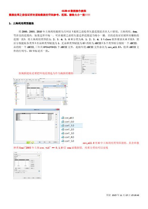
CLUE-S数据操作教程数据处理之前保证所有原始数据的空间参考、范围、栅格大小一致!!!!1、土地利用类型提取将2000、2005、2010年土地利用裁剪为万州区(裁剪之前检查矢量范围是否在人口密度、土地利用、dem、等涉及的范围内,如果边界不统一,可在裁剪之前将矢量边界范围适当缩小一圈,目的是保证后面所有栅格的范围一致),将土地利用类型的1、2、3、4、5、6重分类为0、1、2、3、4、5(clues软件要求从0开始),然后分别提取各类型(有该种类型赋值为1,无该种类型赋值为0)再转为ASCII(各个类型转分别转一个ASCII,总的转一个ASCII,三年共6*3+1*3=21个ASCII文件,起始年的ASCII文件命名为cov_all.0)。
检查ASCII文件的行列号、XY坐标是否一致。
按掩膜提取是要把环境范围选为作为掩膜的栅格cov_all.0用6中土地利用类型直接转,其余单独种类Con("2005年土地rec.tif" == 0,1,0)若con函数报错,用重分类也可以实现2、驱动因子(驱动因子不需要归一化)2.1道路因子(欧氏距离)道路-欧氏距离-转栅格-掩膜(裁剪)-转为ASCII2.2河流因子(欧氏距离)同2.12.3乡镇点因子(欧氏距离)同2.12.4自然村因子(欧氏距离)同2.1注意:做欧氏距离时,环境设置要把范围设置为与边界相同,再用土地利用的栅格掩膜,保证裁剪出来的行列号一致2.5人口密度(人口空间化)2.6 高程Dem-掩膜-转ASCII2.7 坡度DEM-坡度-转ASCII3、回归分析3.1转换为单一记录文件所谓 Logistic 回归,是指因变量为二级计分或二类评定的回归分析,在本文中来分析相关的驱动力与某种土地利用类型的相关关系。
分析前,将水域、耕地、建设用地、林地、园地、未利用地六种地类分别从现状图的栅格文件中提取出来,有该种地类的空间位置设为 1,没有该种地类的空间位置设为 0,再转为 ASCII 文件,与 7种驱动力的 ASCII 码文件仪器用模型自带的 File Converter 软件转化为单一记录的文件,在安装目录新建一个“names.txt空文件”结果自动存于stat.txt文件,这样做的目的是剔除空间中不在研究区域内的空值,然后输入到 SPSS 17.0 中,将每种土地利用类型与 7 种驱动力进行回归分析,得出每种驱动力的β值。
CLUE-S模型在历城区土地利用动态演变模拟中的应用

CLUE运行注意事项

模拟的过程包括以下五个迭代步骤:
(1)确定允许参与变换模拟的栅格。保护用地或其它不允许发生类型转变的栅格将不参与下一步的计算。
(2)根据式(4)计算栅格i适宜土地利用类型u的总概率。
一般就是这几个原因,具体情况具体分析,一定要注意demand文件的准备。
3.在准备驱动文件时注意驱动文件的命名方式:静态因子依次重命名为sclgr0.fil、sclgr1.fil??sclgr8.fil;动态驱动因子:Sclgr#.* (#指解释因子的编码,在模拟期间变化的解释因子,如人口密度,每年都需要准备这样一个模拟的情景假设,*指年)。例如本研究中2000年-2009年人口密度重命名为Sclgr9.1、Sclgr9.2、Sclgr9.3??sclgr9.10.最后把准备好的驱动文件sclgr*.fil和alloc1.reg放入软件安装文件夹下
(3)对各土地利用用类型赋予相同的迭代变量值,按照每一栅格各土地利用类型分布的总概率从大到小对各栅格的土地利用变化进行初次分配。
(4)比较各土地利用类型的初次分配面积和需求面积.若土地利用初次分配的面积大于需求面积,就减小迭代变量的值,反之就增大,然后对土地利用变化进行第二次分配。
(5)重复第2-4步直到各土地利用类型的面积等于需求面积为止,然后保存该年的分配图并开始进行下一年土地利用变化的分配。[15]
进行参数准备的过程中有几点一定要注意(仅是个人感受,如地利用需求文件的时候要特别注意,demand.in*文件中每一行之和要相等(模型运行的时候保留一位小数),否则模型将没有解决方案。如果出错仔细看log文件,里面肯定能分析出原因。
IBMRationalRose操作指南(下)
关系类型
关联
关联是类之间的词法连接,使一个类知道另一个类的公共属性和操作。
关联可以是双向的,但尽量调整为单向,这样可以保证被使用的类可以复用。
关联中被使用的类(即被指向的类)一般是作为另一个的类属性。
依赖
依赖显示一个类引用另一个类。依赖并不对关系的类增加属性,这是跟关联的主要区别。
静态关系
类似输出控制,表示属性是否静态变量
朋友关系
表示Client类能访问Supplier类的非公共属性和操作。
包容
确定聚集关系生成的属性按值还是按引用包容。
限定符
用来缩小关联范围用来设置关联属性。
使用Rose管理关系的技巧
1.设置关系基数的方法:对关联(包括聚集)关系在规范窗口中Role Detail标签中设置;对其它关系,在规范窗口的general标签中设置。
组件类型
1.组件(狭义):具有良好定义接口的软件模块,可以用stereotype字段指定组件类型(如ActiveX、Applet、Application、Dll和Executables等等)。
2.子程序规范:子程序一般是一组子函数(roution)的集合。规范是显示规范。子程序中没有类定义。
3.子程序体。子程序的实现体。
再依赖中,因为一个类不是另一个的属性,所以实现中有三种方法。一是使用全局变量,二是使用本地变量,三是使用函数参数。
包之间也,可以存在依赖性。包A到包B的依赖性表示A中的某些类与B中的某些类有单向关系。
聚集
聚集是强关联。聚集是整体与部分的关系。
实现
显示类与接口、包与接口、组件与接口和用例与用例实现(协作)之间的关系。
第八章关系
介绍类之间的关系。关系是类之间的词法连接,使一个类了解另一个类的属性、操作和关系。
Xcelsius_培训教程
版本号 1.0 日期 2009-7-18 作者 王成 说明 基本完成撰写 email Kelecheng2000@
一、Xcelsius 介绍............................................................................................................................ 5 1.1 Xcelsius 工具说明.............................................................................................................. 5 1.2 Xcelsius 版本介绍.............................................................................................................. 5 1.3 Xcelsius 的向后兼容性...................................................................................................... 5 1.4 Xcelsius 系统介绍.............................................................................................................. 6 1.5 Xcelsius 工作原理的说明.......................................................
ClussCluster包用户说明说明书
Package‘ClussCluster’October12,2022Type PackageTitle Simultaneous Detection of Clusters and Cluster-Specific Genes inHigh-Throughput Transcriptome DataVersion0.1.0Description Implements a new method'ClussCluster'descried in Ge Jiang and Jun Li,``Simultane-ous Detection of Clusters and Cluster-Specific Genes in High-throughput Transcrip-tome Data''(Unpublished).Simultaneously perform clustering analysis and signature gene selection on high-dimensional transcriptome data sets.To do so,'ClussCluster'incorporates a Lasso-type regularization penalty term to the objective function of K-means so that cell-type-specific signature genes can be identified while clustering the cells.Depends R(>=2.10.0)Suggests knitr,rmarkdown(>=1.13)VignetteBuilder knitrImports stats(>=3.5.0),utils(>=3.5.0),VennDiagram,scales(>=1.0.0),reshape2(>=1.4.3),ggplot2(>=3.1.0),rlang(>=0.3.4)License GPL-3Encoding UTF-8LazyData trueRoxygenNote6.1.1NeedsCompilation noAuthor Li Jun[cre],Jiang Ge[aut],Wang Chuanqi[ctb]Maintainer Li Jun<*************>Repository CRANDate/Publication2019-07-0216:30:16UTC12ClussCluster R topics documented:ClussCluster (2)filter_gene (3)Hou_sim (4)plot_ClussCluster (5)plot_ClussCluster_Gap (6)print_ClussCluster (7)print_ClussCluster_Gap (7)sim_dat (8)Index9 ClussCluster Performs simultaneous detection of cell types and cell-type-specificsignature genesDescriptionClussCluster takes the single-cell transcriptome data and returns an object containing cell types and type-specific signature gene setsSelects the tuning parameter in a permutation approach.The tuning parameter controls the L1 bound on w,the feature weights.UsageClussCluster(x,nclust=NULL,centers=NULL,ws=NULL,nepoch.max=10,theta=NULL,seed=1,nstart=20,iter.max=50,verbose=FALSE)ClussCluster_Gap(x,nclust=NULL,B=20,centers=NULL,ws=NULL,nepoch.max=10,theta=NULL,seed=1,nstart=20,iter.max=50,verbose=FALSE)Argumentsx An nxp data matrix.There are n cells and p genes.nclust Number of clusters desired if the cluster centers are not provided.If both are provided,nclust must equal the number of cluster centers.centers A set of initial(distinct)cluster centres if the number of clusters(nclust)is null.If both are provided,the number of cluster centres must equal nclust.ws One or multiple candidate tuning parameters to be evaluated and compared.De-termines the sparsity of the selected genes.Should be greater than1.nepoch.max The maximum number of epochs.In one epoch,each cell will be evaluated to determine if its label needs to be updated.filter_gene3 theta Optional argument.If provided,theta are used as the initial cluster labels of the ClussCluster algorithm;if not,K-means is performed to produce starting clusterlabels.seed This seed is used wherever K-means is used.nstart Argument passed to kmeans.It is the number of random sets used in kmeans.iter.max Argument passed to kmeans.The maximum number of iterations allowed.verbose Print the updates inside every epoch?If TRUE,the updates of cluster label and the value of objective function will be printed out.B Number of permutation samples.DetailsTakes the normalized and log transformed number of reads mapped to genes(e.g.,log(RPKM+1) or log(TPM+1)where RPKM stands for Reads Per Kilobase of transcript per Million mapped reads and TPM stands for transcripts per million)but NOT centered.Valuea list containing the optimal tuning parameter,s,group labels of clustering,theta,and type-specificweights of genes,w.a list containig a vector of candidate tuning parameters,ws,the corresponding values of objectivefunction,O,a matrix of values of objective function for each permuted data and tuning param-eter,O_b,gap statistics and their one standard deviations,Gap and sd.Gap,the result given by ClussCluster,run,the tuning parameters with the largest Gap statistic and within one standard deviation of the largest Gap statistic,bestw and onesd.bestwExamplesdata(Hou_sim)hou.dat<-Hou_sim$xrun.ft<-filter_gene(hou.dat)hou.test<-ClussCluster(run.ft$dat.ft,nclust=3,ws=4,verbose=FALSE)filter_gene Gene FilterDescriptionFilters out genes that are not suitable for differential expression analysis.Usagefilter_gene(dfname,minmean=2,n0prop=0.2,minsd=1)4Hou_simArgumentsdfname name of the expression data frameminmean minimum mean expression for each genen0prop minimum proportion of zero expression(count)for each geneminsd minimum standard deviation of expression for each geneDetailsTakes an expression data frame that has been properly normalized but NOT centered.It returns a list with the slot dat.ft being the data set that satisfies the pre-set thresholds on minumum mean, standard deviation(sd),and proportion of zeros(n0prop)for each gene.If the data has already been centered,one can still apply thefilters of mean and sd but not n0prop. Valuea list containing the data set with genes satisfying the thresholds,dat.ft,the name of dat.ft,andthe indices of those kept genes,index.Examplesdat<-matrix(rnbinom(300*60,mu=2,size=1),300,60)dat_filtered<-filter_gene(dat,minmean=2,n0prop=0.2,minsd=1)Hou_sim A truncated subset of the scRNA-seq expression data set from Hou et.al(2016)DescriptionThis data contains expression levels(normalized and log-transformed)for33cells and100genes. Usagedata(Hou_sim)FormatAn object containing the following variables:x An expression data frame of33HCC cells on100genes.y Numerical group indicator of all cells.gnames Gene names of all genes.snames Cell names of all cells.groups Cell group names.note A simple note of the data set.DetailsThis data contains raw expression levels(log-transformed but not centered)for33HCC cells and 100genes.The33cells belongs to three different subpopulations and exhibited different biological characteristics.For descriptions of how we generated this data,please refer to the paper.Sourcehttps:///geo/query/acc.cgi?acc=GSE65364ReferencesHou,Yu,et al."Single-cell triple omics sequencing reveals genetic,epigenetic,and transcriptomic heterogeneity in hepatocellular carcinomas."Cell research26.3(2016):304-319.Examplesdata(Hou_sim)data<-Hou_sim$xplot_ClussCluster Plots the results of ClussClusterDescriptionPlots the number of signature genes against the tuning parameters if multiple tuning parameters are evaluated in the object.If only one is included,then plot_ClussCluster returns a venn diagram and a heatmap at this particular tuning parameter.Usageplot_ClussCluster(object,m=10,snames=NULL,gnames=NULL,...)top.m.hm(object,m,snames=NULL,gnames=NULL,...)Argumentsobject An object that is obtained by applying the ClussCluster function to the data set.m The number of top signature genes selected to produce the heatmap.snames The names of the cells.gnames The names of the genes...Addtional parameters,sent to the methodDetailsTakes the normalized and log transformed number of reads mapped to genes(e.g.,log(RPKM+1) or log(TPM+1)where RPKM stands for Reads Per Kilobase of transcript per Million mapped reads and TPM stands for transcripts per million)but NOT centered.If multiple tuning parameters are evaluated in the object,the number of signature genes is computed for each cluster and is plotted against the tuning parameters.Each color and line type corresponds to a cell type.If only one tuning parameter is evaluated,two plots will be produced.One is the venn diagram of the cell-type-specific genes,the other is the heatmap of the data with the cells and top m signature genes.See more details in the paper.Valuea ggplot2object of the heatmap with top signature genes selected by ClussClusterExamplesdata(Hou_sim)<-ClussCluster(Hou_sim$x,nclust=3,ws=c(2.4,5,8.8))plot_ClussCluster(,m=5,snames=Hou$snames,gnames=Hou$gnames)plot_ClussCluster_Gap Plots the results of ClussCluster_GapDescriptionPlots the gap statistics and number of genes selected as the tuning parameter varies.Usageplot_ClussCluster_Gap(object)Argumentsobject object obtained from ClussCluster_Gap()print_ClussCluster7 print_ClussCluster Prints out the results of ClussClusterDescriptionPrints out the results of ClussClusterUsageprint_ClussCluster(object)Argumentsobject An object that is obtained by applying the ClussCluster function to the data set.print_ClussCluster_GapPrints out the results of ClussCluster_Gap Prints the gap statisticsand number of genes selected for each candidate tuning parameter.DescriptionPrints out the results of ClussCluster_Gap Prints the gap statistics and number of genes selected for each candidate tuning parameter.Usageprint_ClussCluster_Gap(object)Argumentsobject An object that is obtained by applying the ClussCluster_Gap function to the data set.8sim_dat sim_dat A simulated expression data set.DescriptionAn example data set containing expressing levels for60cells and200genes.The60cells belong to4cell types with15cells each.Each cell type is uniquely associated with30signature genes,i.e.,thefirst cell type is associated with thefirst30genes,the second cell type is associated withthe next30genes,so on and so forth.The remaining80genes show indistinct expression patterns among the four cell types and are considered as noise genes.Usagedata(sim_dat)FormatA data frame with60cells on200genes.ValueA simulated dataset used to demonstrate the application of ClussCluster.Examplesdata(sim_dat)head(sim_dat)Index∗datasetsHou_sim,4sim_dat,8ClussCluster,2ClussCluster_Gap(ClussCluster),2filter_gene,3Hou_sim,4plot_ClussCluster,5plot_ClussCluster_Gap,6print_ClussCluster,7print_ClussCluster_Gap,7sim_dat,8top.m.hm(plot_ClussCluster),59。
- 1、下载文档前请自行甄别文档内容的完整性,平台不提供额外的编辑、内容补充、找答案等附加服务。
- 2、"仅部分预览"的文档,不可在线预览部分如存在完整性等问题,可反馈申请退款(可完整预览的文档不适用该条件!)。
- 3、如文档侵犯您的权益,请联系客服反馈,我们会尽快为您处理(人工客服工作时间:9:00-18:30)。
Course material Peter Verburg
January 2010
CLUE model - background
Introduction The Conversion of Land Use and its Effects modelling framework (CLUE) was developed to simulate land use change using empirically quantified relations between land use and its driving factors in combination with dynamic modelling of competition between land use types. The model was developed for the national and continental level and applications for Central America, Ecuador, China and Java, Indonesia are available. For study areas with such a large extent the spatial resolution for analysis was coarse and, as a result, each land use is represented by assigning the relative cover of each land use type to the pixels. Land use data for study areas with a relatively small spatial extent is often based on land use maps or remote sensing images that denote land use types respectively by homogeneous polygons or classified pixels. This results in only one dominant land use type occupying one unit of analysis. Because of the differences in data representation and other features that are typical for regional applications, the CLUE model cannot directly be applied at the regional scale. Therefore the modelling approach has been modified and is now called CLUE-S (the Conversion of Land Use and its Effects at Small regional extent). CLUE-S is specifically developed for the spatially explicit simulation of land use change based on an empirical analysis of location suitability combined with the dynamic simulation of competition and interactions between the spatial and temporal dynamics of land use systems. More information on the development of the CLUE-S model can be found in Verburg et al. (2002) and Verburg and Veldkamp (2003). The more recent versions of the CLUE model: Dyna-CLUE (Verburg and Overmars, 2009) and CLUE-Scanner include new methodological advances. Model structure The model is sub-divided into two distinct modules, namely a non-spatial demand module and a spatially explicit allocation procedure (Figure 1). The non-spatial module calculates the area change for all land use types at the aggregate level. Within the second part of the model these demands are translated into land use changes at different locations within the study region using a raster-based system. The userinterface of the CLUE-S model only supports the spatial allocation of land use change. For the land use demand module different model specifications are possible ranging from simple trend extrapolations to complex economic models. The choice for a specific model is very much dependent on the nature of the most important land use conversions taking place within the study area and the scenarios that need to be considered. The results from the demand module need to specify, on a yearly basis, the area covered by the different land use types, which is a direct input for the allocation module.
3
Figure 2. Overview of the information flow in the CLUE-S model Land use type specific conversion settings Land use type specific conversion settings determine the temporal dynamics of the simulations. Two sets of parameters are needed to characterize the individual land use types: conversion elasticities and land use transition sequences. The first parameter set, the conversion elasticities, is related to the reversibility of land use change. Land use types with high capital investment will not easily be converted in other uses as long as there is sufficient demand. Examples are residential locations but also plantations with permanent crops (e.g., fruit trees). Other land use types easily shift location when the location becomes more suitable for other land use types. Arable land often makes place for urban development while expansion of agricultural land occurs at the forest frontier. An extreme example is shifting cultivation: for this land use system the same location is mostly not used for periods exceeding two seasons as a consequence of nutrient depletion of the soil. These differences in behaviour towards conversion can be approximated by conversion costs. However, costs cannot represent all factors that influence the decisions towards conversion such as nutrient depletion, esthetical values etc. Therefore, for each land use type a value needs to be specified that represents the relative elasticity to change, ranging from 0 (easy conversion) to 1 (irreversible change). The user should decide on this factor based on expert knowledge or observed behaviour in the recent past. The second set of land use type characteristics that needs to be specified are the land use type specific conversion settings and their temporal characteristics. These settings are specified in a conversion matrix. This matrix defines: To what other land use types the present land use type can be converted or not (Figure 3).