软件使用说明-PCPDFWIN
材料分析方法 第七章c1

「Back」的功用: 关闭“Search window”回到“PCPDFWIN”画 面。
PDF检索实例之一
目标:找出矿物 calcite(方解石)的PDF数据。
<例1>
步骤:「Search」「Names」 「Mineral Names」键 入“calcite” 。检索结果有66笔,执行「Search Result」, 选择 PDFNumber #24-0027 然后按“OK”。
「Select Elements」的“Inclusive”功能:
将数据库中具有选定元素的所有化合物呈现出來。 例:选择B(硼)和O(氧)则检索结果有2816笔。
Elements选项的「Element with Atom Count」的功能: 提供一个对话框,键入某一化学式,卡片库中只要有符 合该化学式的结果均呈现出來。例:Ca4 出现439笔数据。
开启PCPDFWIN,出现此窗口, 在「File」选项中,可依据个人需 要对数据库进行设定。
若已知「PDF Number」,可直 接输入以获取所需资料。
点击「Search」选项出现 此画面,可进行查询功能。
使用上若有任何疑难,可在 「Help」菜单中寻找答案。
在Search Window里的「Search Files」 选项,提供建立新文件、打开旧文件、 和存档以及另存新文件等功能。
Names选项的「Inorganic or Common Names」功能:
使用者可用“化学名”或“俗名”针对无机物质作搜索。
Names的「Mineral Names」功能: 可用“矿物名”全称或者全称的一部分进行查找。
Names的「Mineral Groups」功能:
使用者可自行选择矿物族的类别进行搜索。
FXGPWIN编程软件使用

图09 帮助文件界面
一 程序编制 1.编制语言的选择 FXGPWIN软件提供三种编程语言,分 别是:梯形图、语句表和功能逻辑图 (SFC)。打开“视图”菜单,如图10所 示。 选择对应的编程语言。
图10 编制语言选择界面
• 2.采用梯形图编写程序 • (1)按以上步骤选择梯形图编程语言。选 择“视图”菜单下的“工具栏”,“状态 栏”,“功能键”和“功能图”子菜单, 如图11所示。
图21 寄存器数据传送界面
• 2.“选项”菜单的使用 • “选项”菜单的内容如图22所示。
图22 “选项”菜单界面
• (1)可编程控制器EPROM的处理 • 打开“EPROM传送”子菜单有三项内容:“读 入”,“写出”和“核对”。按“读入”键,即 可从可编程控制器读出EPROM的内容。按“写 出”键,即可将编写的程序写入可编程控制器中。 “核对”键用于验证编写的程序和EPROM中的 内容是否一致。 • (2)单击“选项”菜单下的“字体”子菜单,即 可设置字体式样、大小等有关内容,如图23所示。 • (3)“窗口”菜单的使用 • 双击“窗口”菜单下的“视图顺排”子菜单,就 可层铺编程环境。双击“窗口水平排列”子菜单, 就可水平铺设编程环境。双击“窗口垂直排列” 子菜单,就可垂直铺设编程环境。
图03 端口设置菜单窗口界面 选择好串行口后,打开图02“PLC”菜单下的“程序 读入”子菜单,即可进入如图04所示的界面。正确 选择可编程控制器型号,按确认键后等待几分钟, 可编程控制器中的程序即下载到计算机的FXGPWIN 文件夹中。程序下载后界面如图05所示。
图04 PLC型号选择界面
图05 PLC程序下载后界面
图07 打开新文件界面
图08 编制程序界面
• 5.设置页面和打印 • 打开“文件”菜单下的“页面设置”子菜单即可 进行编程页面设置。打开“文件”菜单下的“打 印机设置”子菜单,即可进行打印设置。 • 6.退出主程序 • 打开“文件”菜单下的“退出”子菜单或按右上 角的×按键,即可退出主程序。 • 7.帮助文件的使用 • 打开“帮助”菜单下的“索引”子菜单,寻找所 需帮助的目录名,如图09所示,双击目录名即可 进入帮助文件的内容。“帮助”菜单下的“如何 使用帮助”告诉你如何使用此帮助文件
PcPDFwin详解(看完就会了,已转为简体)
Search Window的「Elements」选项的「Number of Elements」 指令,其功用在于依据使用者的元素数目之限制,仅呈现相对应 的样本数据,例:选择3Elements 则在所有的样本数据里,恰 巧只含有3种不同元素数目的样本才会出现,此指令和「Select Elements」指令,一起结合使用是极有用的方式。
开启数据库后,出现此窗口画面,在「File」 选项中,可依据使用者个别的需要对数据库 做使用上的设定。
若已知「PDF ID Number」时, 可直接输入以获取所需之数据。
点选「Search」项目即出现此画 面,可进行查询的功能。
若读者在使用上有任何疑难,也可 自行在「Help」选单内容里寻找答 案。
接着执行「Subfiles」「Explosive」,则检索结果由3128笔筛选 至剩9笔。
再进一步执行「Misc.」「Melting Point」,键入上限“174”下限 “173”然后按OK。
最后的检索结果只有1笔,将结果选取然后执行「Search Result」即 得到化合物为“Ferrocene” ( C10H10Fe )。
Misc.选单的「LongLines」的功能为:选取三条最长的面距(d-spacing) 中的一条作为搜寻的准则。
Misc.选单的「Reduced Cell Axis」的功能为:选取“缩减的晶胞 轴”(Reduced Cell Axis)作为搜寻的准则,单位是埃 (Angstroms)。
Misc.选单的「Density」功能为:提供一个对话盒,读者用已测量出的密 度作为检索数据库的策略,单位是(cm3/g)。若无有效的测量密度值时, 再行使用纯计算的密度值代替。
数据库简介: 本数据库由International Centre for Diffraction Data出版,收录各种天 然矿物、人工化合物 (有机及无机)、元素及合金等之X-ray粉末绕射数据,对 于进行未知物辨识或材料成份分析非常有帮助,目前馆藏为 sets 1-47,可以 输入PDF number、Mineral Name、Chemical Name、3 Strongest Lines等字段 查询,并提供检索结果打印及存档。 (Power Diffraction File)是单一相X光粉末绕射样本的收集,其维护和分 类工作由国际绕射资料中心(ICDD)提供。每笔数据以表格的形式呈现,包括 特定的面与面之间的距离、对应的相对强度、米勒指数、结晶系统、密度等均 涵盖其中。
PSVIEW软件使用说明书_NEW

PSViewPS系列数字式保护调试分析软件使用说明书国电南京自动化股份有限公司PS系列数字式保护调试分析软件PSView使用说明书编写尹军张云审核马文龙批准郭效军V2.12000年4月国电南京自动化股份有限公司*本公司保留修改的权力目次1.软件介绍 (1)2.用户许可协议 (1)3.安装与卸载 (1)3.1 运行环境 (1)3.2 安装 (2)3.3 卸载 (2)4.使用说明 (3)4.1 功能菜单 (3)4.2 使用系统工具栏 (5)4.3 系统功能以及辅助功能 (7)4.3.1保护CPU的重新连接与刷新 (7)4.3.2保护CPU的切换 (7)4.3.3运行/调试模式切换 (7)4.3.4通讯参数设置和通讯原码查看 (8)4.3.5报告的打开,保存,打印等文件功能 (9)4.4 主要调试分析功能的相关操作 (10)4.4.1 整定值查询,修改,固化 (10)4.4.2 运行定值区切换 (11)4.4.3 保护动作事件及开关变位事件跟踪查询 (11)4.4.4 故障录波数据查询,分析 (13)4.4.5开入量定时查询 (16)4.4.6采样通道有效值,相角,直流偏移查询及增益系数查看 (16)4.4.7实时采样数据查询 (16)4.4.8开出量跳合测试 (17)4.4.9 内存单元数据查询及修改 (17)4.4.10 内部定值 (17)4.4.11 保护配置信息浏览 (17)5. 软件版本升级 (18)PS系列数字式保护调试分析软件PSView使用说明书 1 1.软件介绍PS系列数字式保护调试分析软件(PSView)是为配合我公司出品的PSL620系列,PSL600系列等数字式继电保护装置编写的调试分析软件,不但能够完成人机对话的功能,还能对保护录波数据以及保护内部各元件动作过程进行分析。
PS系列数字式保护调试分析软件,以下简称(PSView软件)兼容Windows95,Windows98和Windows2000操作系统,操作简单方便。
plotwidgets 0.5.1 软件包说明书
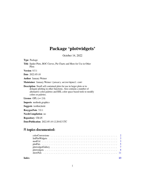
Package‘plotwidgets’October14,2022Type PackageTitle Spider Plots,ROC Curves,Pie Charts and More for Use in OtherPlotsVersion0.5.1Date2022-05-10Author January WeinerMaintainer January Weiner<************************>Description Small self-contained plots for use in larger plots or todelegate plotting in other functions.Also contains a number ofalternative color palettes and HSL color space based tools to modifycolors or palettes.License GPL(>=2.0)Imports methods,graphicsSuggests testthat,knitrRoxygenNote5.0.1NeedsCompilation noRepository CRANDate/Publication2022-05-1012:20:02UTCR topics documented:colorConversions (2)listPlotWidgets (3)modCol (3)plotPals (5)plotwidgetGallery (7)plotwidgets (8)showPals (11)Index1312colorConversions colorConversions Convert colors from and to RGB and HSL formatsDescriptionConvert colors from and to RGB and HSL formatsUsagecol2rgb.2(col)col2hsl(col)hsl2col(hsl)rgb2col(rgb)rgb2hsl(rgb)hsl2rgb(hsl)Argumentscol a character vector with colors to convert(palette)hsl a numeric matrix with three or four rows(hue,saturation,luminosity and alpha) rgb a numeric matrix with three or four rows(red,green,blue and alpha)DetailsThese functions convert between RGB and HSL color spaces,and character vectors which contain color names or hash-encoded RGB values("#FFCC00").All functions support an alpha channel.For example,unlike the grDevices::col2rgb,col2rgb.2 returns a matrix with four rows:three for R,G and B channels and one for the alpha channel. Valuecol2rgb.2and col2hsl return a four-row matrix.rgb2col and hsl2col return a character vector.Functions•col2rgb.2:Convert a character vector of color names(palette)to a matrix with RGB values •col2hsl:Convert a character vector of color names(palette)to a matrix with HSL values•hsl2col:Convert hsl matrix(3or4row)to character vector of color names•rgb2col:Convert rgb matrix(3or4row)to character vector of color names•rgb2hsl:Convert a3-or4-row matrix of RGB(A)values to a matrix of HSL(A)values•hsl2rgb:Convert a matrix of HSL values into a matrix of RGB valueslistPlotWidgets3 See AlsomodCol,modhueCol,darkenCol,saturateColExampleshaze<-plotPals("haze")col2rgb(haze)col2hsl(haze)listPlotWidgets List available plot widgetsDescriptionList available plot widgetsUsagelistPlotWidgets()DetailsSimply print out all available wigdets.A list containing the widget function is returned invisibly.ValueInvisibly returns a named list of widget functionsExampleslistPlotWidgets()modCol Modify colorsDescriptionModify colors by shading,saturating and changing hue4modCol UsagemodCol(col,darken=0,saturate=0,modhue=0)saturateCol(col,by=0)darkenCol(col,by=0)modhueCol(col,by=0)contrastcol(col,alpha=NULL)Argumentscol a character vector of colors(palette)to modify–a character vectordarken Use negative values to lighten,and positive to darken.saturate Use negative values to desaturate,and positive to saturatemodhue Change the hue by a number of degrees(0-360)by parameter for the saturateCol,darkenCol and modhueCol functionsalpha alpha value(from0,transparent,to255,fully opaque)DetailsThis function use the HSL(hue,saturation,luminosity)scheme to modify colors in a palette.modCol is just a wrapper for the other three functions allowing to modify three parameters in one go.saturateCol,darkenCol and modhueCol modify the saturation,luminosity and hue in the HSL color model.contrastcol()returns black for each light color(with L>0.5)and white for each dark color(with L<0.5).Valuea character vector containing the modified paletteFunctions•saturateCol:Change the saturation of a color or palette by a fraction of"by"•darkenCol:Modify the darkness of a color or palette(positve by-darken,negative by–lighten)•modhueCol:Modify the hue of a character vector of colors by by degrees•contrastcol:Return white for dark colors,return black for light colorsplotPals5Examplesplot.new()##Loop over a few saturation/lightess valuespar(usr=c(-0.5,0.5,-0.5,0.5))v<-c(10,9,19,9,15,5)pal<-plotPals("zeileis")for(sat in seq.int(-0.4,0.4,length.out=5)){for(lgh in seq.int(-0.4,0.4,length.out=5)){cols<-saturateCol(darkenCol(pal,by=sat),by=lgh)wgPlanets(x=sat,y=lgh,w=0.16,h=0.16,v=v,col=cols)}}axis(1)axis(2)title(xlab="Darkness(L)by=",ylab="Saturation(S)by=")##Now loop over huesa2xy<-function(a,r=1,full=FALSE){t<-pi/2-2*pi*a/360list(x=r*cos(t),y=r*sin(t))}plot.new()par(usr=c(-1,1,-1,1))hues<-seq(0,360,by=30)pos<-a2xy(hues,r=0.75)for(i in1:length(hues)){cols<-modhueCol(pal,by=hues[i])wgPlanets(x=pos$x[i],y=pos$y[i],w=0.5,h=0.5,v=v,col=cols)}pos<-a2xy(hues[-1],r=0.4)text(pos$x,pos$y,hues[-1])plotPals Return all or selected color palettesDescriptionReturn all or selected color palettes from the plotwidget palette setUsageplotPals(pal=NULL,alpha=1,drop.alpha=TRUE)Argumentspal Name of the palette(s)to return6plotPalsalpha Control transparency -set alpha channel to alpha (0-fully transparent,1-fully opaque)drop.alphaIf true,and if alpha is NULL,the "FF"string of the alpha channel will not be attached to the produced RGB codesDetailsThe plotwidgets package contains a number of predefined palettes,different from those in RColor-Brewer.•default :a standard,relatively safe (see below)palette•safe :safe for color blind persons,based on Wang B."Points of view:Color blindeness",Nature Methods 8,441(2011)•neon :a bright palette suitable for drawing on dark backgrounds •pastel :a dimmed pastel palette •haze :very delicate pastel colors •dark :same hues as haze,but much darker •grey :different shades of grey•alphabet :based on "A colour alphabet..."by Paul Green-Armytage •few :a palette based on Stephen Few’s book •zeileis :based on Zeileis et al.2009•vizi :automatically generated palette12345678910111213141516171819123456781234567891234567891011121314151612345678910123456789101234567891234567891011121314151617181920212223242512345678912345678910111213141516171819202122232412345678910defaultsafeneon pastelhaze darkhaze grey alphabetfewzeileis viziYou can get all the names of palettes with names(plotPals()),and showcase them with show-Palettes().Furthermore,you can use the pal parameter to plotwidgetGallery to see how this palette looks like with different plot widgets.ValueEither a list of palettes,or (if only one palette was selected)a character vector with colors See Alsocol2rgb.2,rgb2col ,hsl2col ,col2hsl ,modCol ,modhueCol ,darkenCol ,saturateColUsageplotwidgetGallery(theme="default",pal=NULL,...)Argumentstheme sets both the palette and a suitable bakckground(e.g.dark for"neon") pal color palette to use(a character vector with colors)...all subsequent parameters will be passed to the plotWidget()function. DetailsplotwidgetGallery()simply draws all available plot widgets on a single plot.ValueInvisibly returns the example data used to generate the plotsExamplesplotwidgetGallery()##automatically set black bgplotwidgetGallery(theme="neon")##yuck,ugly:plotwidgetGallery(pal=c("red","#FF9900","blue","green","cyan","yellow")) ##much better:plotwidgetGallery(pal=plotPals("pastel",alpha=0.8))plotwidgets Plot widgetsDescriptionA collection of plotting widgets(pie charts,spider plots etc.)UsageplotWidget(type="pie",x=0.5,y=0.5,w=1,h=1,v,col=NULL,border=NA,new=FALSE,aspect=1,...)wgPie(x=0.5,y=0.5,w=1,h=1,v,col=NULL,border=NA,new=FALSE,res=100,aspect=1,adj=0,labels=NULL,label.params=NULL)wgRing(x=0.5,y=0.5,w=1,h=1,v,col=NULL,border=NA,new=FALSE,res=100,aspect=1,adj=0,start=0.5,labels=NULL,label.params=NULL)wgPlanets(x=0.5,y=0.5,w=1,h=1,v,col=NULL,border=NA,new=FALSE,res=100,aspect=1,adj=0,labels=NULL,label.params=NULL)wgBurst(x=0.5,y=0.5,w=1,h=1,v,col=NULL,border=NA,new=FALSE,res=100,aspect=1,adj=0,max=NULL,labels=NULL,label.params=NULL)wgRug(x=0.5,y=0.5,w=1,h=1,v,col=NULL,border=NA,labels=NULL,label.params=NULL,new=FALSE,aspect=NULL,horizontal=TRUE,rev=FALSE)wgBarplot(x=0.5,y=0.5,w=1,h=1,v,col=NULL,border=NA,labels=NULL,label.params=NULL,new=FALSE,aspect=NULL,max=NULL)wgBoxpie(x=0.5,y=0.5,w=1,h=1,v,col=NULL,border=NA, labels=NULL,label.params=NULL,new=FALSE,aspect=1,grid=3)wgRoccurve(x=0.5,y=0.5,w=1,h=1,v,col=NULL,border=NA,new=FALSE,fill=FALSE,lwd=1,aspect=1)wgSpider(x=0.5,y=0.5,w=1,h=1,v,col=NULL,border=NA,new=FALSE,min=NA,max=NA,bels=FALSE,fill=FALSE,lwd=1,aspect=1)Argumentstype what kind of plot.To list all available plot types,use listPlotWidgets.Instead of the canonical name such as"wgSpider",you can simply use"spider"x,y coordinates at which to draw the plotw,h width and height of the plotv sizes of the slicescol character vector with colors(palette).A default palette is chosen if the argument is NULLborder color of the e NA(default)for no border,and NULL for a border in the par("fg")color.No effect in spider plots.new Whether to call plot.new()before drawing the widgetaspect the actual ratio between screen width and screen height.Parameters w and h will be scaled accordingly....Any further arguments passed to plotting functionsres for pies,rings,planets and bursts:resolution(number of polygon edges in a full circle)adj for spider plots,burst plots,planet plots and pies:adjust the start by"adj"de-grees.For example,to turn the plot clockwise by90degrees,use adj=90 labels character vectorlabel.params a named list with arguments passed to text()for drawing labels(e.g.cex,col etc.)start For ring plots,the inner radius of the ringmax For burst plots–a maximum value used to scale other values to make different plots comparable.For spider plots:the maximum of the scale on spider plotspikes.horizontal for rug plots:whether the stacked bar should be horizontal(default),or vertical rev logical,for rug plots:right to left or top to bottom rather than the default left to right or bottom to topgrid boxpie only:the grid over which the areas are distributed.Should be roughly equal to the number of areas shown.fill for spider plots and roc curves:whether to drawfilled polygons rather than lines lwd Line width to usemin For spider plots:the minimum of the scale on spider plot spikesbels For spider plots:labels for the scale ticksDetailsA widget here is a mini-plot which can be placed anywhere on any other plot,at an area specifiedby the center point coordinates x and y,and width and height.The widgets do not influence the layout of the plot,or change any parameters with par();it only uses basic graphic primitives for maximal compatibility.The plotWidget()function is a generic to call the available widgets from one place.Any widget-specific parameters are passed on through the ellipsis(...).See the documentation for specific widgets for more e the functions listPlotWidgets and plotwidgetGallery to see available widgets.The pie function draws a simple pie chart at specified coordinates with specified width,height and color.The rug function draws a corresponding rug plot,while boxpie creates a"rectangular pie chart"that is considered to be better legible than the regular pie.Functions•wgPie:pie()draws a pie chart with width w and height h at coordinates(x,y).The angle width of the slices is taken from the numeric vector v,and their color from the character vector col.Note that one of the main goals of the plotwidget package is to give sufficient alternatives to pie charts,hoping to help eradicate pie charts from the surface of this planet.•wgRing:A pie with the center removed.•wgPlanets:Produces a circular arrangement of circles,which vary in their size proportionally to the values in v.•wgBurst:Burst plots are similar to pies.However,instead of approximating numbers by arc length,wgBurst approximates by area,making the pie slices stand out from the plot in the process.•wgRug:A stacked,horizontal or vertical bar plot.•wgBarplot:A minimalistic bar e the max paramter to scale the bars on several differ-ent widgets to the same value.•wgBoxpie:Rectangular pies are thought to represent information better than pies.Here,the values in v correspond to areas rather than angles,which makes it easier to interpret it visually.•wgRoccurve:This is one of two wigets that take use a different data type.wgRoccurve takes either a vector of T/F values,or a list of such vectors,and draws a ROC curve for each of these vectors.•wgSpider:Spider plots can illustrate multivariate data.Different spikes may illustrate dif-ferent variables,while different lines correspond to different samples–or vice versa.Conse-quently,wgSpider accepts either a vector(for a single line)or a matrix(in which each column will correspond to a single line on the plot).The length of the vector(or the number of rows in the matrix)corresponds to the number of spikes on the spider plot.See AlsowgPie,wgBoxpie,wgSpider,wgRug,wgBurst,wgRing,wgBarplot,wgPlanets,wgRoccurveExamples#demonstration of the three widgetsplot.new()par(usr=c(0,3,0,3))v<-c(7,5,11)col<-plotPals("safe")b<-"black"wgRug(0.5,1.5,0.8,0.8,v=v,col=col,border=b)wgPie(1.5,1.5,0.8,0.8,v=v,col=col,border=b)wgBoxpie(2.5,1.5,0.8,0.8,v=v,col=col,border=b)#using pie as plotting symbolplot(NULL,xlim=1:2,ylim=1:2,xlab="",ylab="")col<-c("#cc000099","#0000cc99")for(i in1:125){x<-runif(1)+1y<-runif(1)+1wgPie(x,y,0.05,0.05,c(x,y),col)}#square filled with box piesn<-10w<-h<-1/(n+1)plot.new()for(i in1:n)for(j in1:n)wgBoxpie(x=1/n*(i-1/2),y=1/n*(j-1/2),w,h,v=runif(3),col=plotPals("zeileis"))showPals Demonstrate selected palettesDescriptionShow a plot demonstrating all colors in the provided palettesUsageshowPals(pal=NULL,numbers=T)Argumentspal Either a character vector of colors or a list of character vectors numbers On each of the colors,show a numberExamples##Show all palettes in plotwidgetshowPals(plotPals())##Show just a few colorsshowPals(c("red","green","blue"))Indexcol2hsl,6col2hsl(colorConversions),2col2rgb.2,6col2rgb.2(colorConversions),2 colorConversions,2contrastcol(modCol),3darkenCol,3,6darkenCol(modCol),3hsl2col,6hsl2col(colorConversions),2hsl2rgb(colorConversions),2 listPlotWidgets,3,10modCol,3,3,6modhueCol,3,6modhueCol(modCol),3plotPals,5plotWidget(plotwidgets),8 plotwidgetGallery,6,7,10 plotwidgets,8plotwidgets-package(plotwidgets),8 rgb2col,6rgb2col(colorConversions),2rgb2hsl(colorConversions),2 saturateCol,3,6saturateCol(modCol),3showPals,11wgBarplot,10wgBarplot(plotwidgets),8 wgBoxpie,10wgBoxpie(plotwidgets),8wgBurst,10wgBurst(plotwidgets),8wgPie,10wgPie(plotwidgets),8wgPlanets,10wgPlanets(plotwidgets),8wgRing,10wgRing(plotwidgets),8wgRoccurve,10wgRoccurve(plotwidgets),8wgRug,10wgRug(plotwidgets),8wgSpider,10wgSpider(plotwidgets),8 13。
软件使用说明-PCPDFWIN

Search Window中的「Logical Operators」選 項,提供3種布林邏輯運算功能,可於搜尋 輸出結果上做使用。
Search Window畫面的「Subfiles」選項 有諸多選擇,讀者可在多種的化合物類 別裡做限定,以幫助搜尋。
Search Window的「Elements」選項的「Number of Elements」 指令,其功用在於依據使用者的元素數目之限制,僅呈現相對應 的樣本資料,例:選擇 3 Elements 則在所有的樣本資料裡,恰 巧只含有3種不同元素數目的樣本才會出現,此指令和「Select Elements」指令,一起結合使用是極有用的方式。
`
Misc.選單的「Reduced Cell Volume」的功能為:選取“縮減的晶胞體 積”(Reduced Cell Volume)作為搜尋的準則,單位是立方埃(Cubic Angstroms)。
Misc.選單的「Reference」功能為:讀者使用“期刊引用文獻”作為搜尋基 礎,功能選項有“引用文獻的作者”(Authors)、該“期刊代碼” (Coden)、 該“期刊出版年份”(Year)等不同操作供讀者自行選擇使用。
「Select Elements」的“Inclusive”功能為:資料庫的全部樣本化合物 中,只要具有使用者所選定的元素,均呈現出來。例:選擇B(硼) 和O(氧)則檢索結果有2514筆,由於此方式所得筆數太多,需以布 林邏輯操作做進一步的篩選。
「Select Elements」的“Just”功能為:類似“Only”的功用,但包括個 別的單一元素態。例:選擇B(硼)和O(氧)則檢索結果有48筆。
本資?庫由internationalcentrefordiffractiondata出版收?各種天然礦物人工化合物有機及無機元素及合?等之xray粉末繞射資?對于進?未知物辨?或材?成份分析非常有幫助目前館藏為sets147可以輸入pdfnumbermineralnamechemicalname3strongestlines等?位查詢並提供檢?結果?印及存檔
proface编程软件实践操作手册2
Logging 功能 配方功能
22 Base(50) 17 Base(60)
Base(70) 16
第四章 多语言在线切换
• 多语言的应用 • 多语言字符串表
4.1
多语言的应用
本章将说明如何使用多语言在线切换功能。
4.1多语言的应用
要点! 1. 多语言显示切换功能需要在GP377/77R/2000系列上,GP-PRO/PBIII V6.O版以上软件支持。 2.普通的文本内容或部件的标签,可以用字符串表的索引编号方式进行处理,这样可以非常方便地在运行时 改变字符串表,从而实现多语言的在线切换,不用分别对不同语言重复做画面。
(3) 触发器设置的内容 (时间方法)
①Start Time: 设置开始日志的时间
Duration: 设置日志的持续时间。从开始到结束期 间的日志数据作为一个时期内的一个块进行处理。 Read Count: 设置为块收集数据的频率。结束时 间自动取决于设置的频率。
5.1显示记录的数据
1 2
②
Data Logging Auth. Bit Address: 设置位地址以允许日志。如果指定的位地址为[OFF],则不 会有数据记录,即使到了开始处理的时间也是如此。 Block’s Finish Bit Address: 设置记录了一个块时[ON]的位地址。
(例如:20个字的数据重复100次(一块)的大小约为5KB) 请参见[标签参考手册]以获得关于此公式的详细说明。
・关于数据收集画面 1
①
收集的数据显示在画面上。
②
触摸以滚动收集数据列表。
③
每次在触摸时会收集数据。
④
每次收集了一组数据后就会变亮。
⑤
收集了用于曾经设置频率的数据时就会发亮。
FXGPWIN使用说明书
FXGPWIN软件使用说明书——by 施祺本说明主要用图片演示操作,有图有真相~仅供参考。
一.生成梯形图软件打开后入图1。
主界面按钮中,转换按钮比较重要,相当于IDE中的编译、链接操作。
梯形图画好以后要重新转换才能替换原来的指令。
图1 软件启动界面点击新文件,要求对PLC选型,本实验使用FX1S型PLC。
如图2。
图2 PLC选型建立好的新文件如图3,包含梯形图和指令语句表。
指令语句表是不需要写的,所谓转换,就是更新指令语句表。
图3 建立新文件二.元件放置实验中常用到的元件在功能图对话框(视图->功能图)中都能找到,常用元件注释如图4。
图4 功能图对话框放置触点和继电器等元件,点击相应按钮,输入对应参数即可。
如图5。
图5 放置触点要看元件的使用范围,点击参照,从可选元件范围中选定一种,并定义使用几号元件。
如图6。
图6 元件说明生成好的元件如图7,待转换的部分自动标灰色。
灰色区域可以自由跨行复制,而转换后只能单行复制,因此如有相同的模块,应在转换前复制好,以节省时间。
图7 生成元件三.定时器和计数器定时器定义格式如图8,T代表定时器,K代表延时时间。
这里,延时时间=0.1*10=1s。
串联常开触点并联常开触点串联常闭触点并联常闭触点继电器指令框添加并联竖线写入PLC 删除竖线图8 定时器计数器定义格式如图9,需要分别定义复位端和输入端。
图9 计数器经过转换的元件及指令语句表如图10。
(图示程序仅供参考原件外形)图10 经过转换的元件及指令语句表实验内容基本只需要以上操作就可以完成了。
要连接PLC,先将PLC核心上的开关拨到烧写模式,点功能图对话框上的写出按钮(或者:PLC->传送->写出)。
写出前先转换,否则程序不更新。
由于本软件产生于Windows3.1年代,是近20年前的软件,难免有许多Bug,用户界面不够友好,请大家耐心些。
需要注意的是,文件在保存前一定要先转换,否则保存不上。
XRD测试
物相分析的基本原理
任何一种结晶物质都具有特定的晶体结构
在一定波长的X射线照射下,不同的晶体结构产生完全 不同的衍射花样
不可能有两种晶体结构的衍射花样完全相同 多相试样的衍射图谱不因为存在多相而产生变化,只是
各自衍射花样的机械叠加
物相分析的方法
利用布拉格公式2dsinθ= λ ,通过计算机将图谱中的衍 射峰位转换成d值,衍射强度按百分比计算I(I=I测/I最 大*100),得出只与相的特征有关而与仪器、波长无 关的d-I列表,代替实际图谱。
Educational:
1071
Explosives:
345
Forensic:
3767
Intercalates:
130
Ionic Conductors:
43
Metals & Alloys:
17153
Minerals:
8863
NBS:
2098
Pharmaceutical:
1483
Pigments:
342
到1963年共出版13集,以后按每年1集的速度递增 1969年成立了“粉末衍射标准联合委员会”,简称为
JCPDS的国际组织,由它负责编辑和出版粉末衍射卡片, 称为PDF卡片,至2004年共54集,每集约2000张。另有 通过计算机计算得出的10多集(60-79)
PDF资料库
由 International Centre for Diffraction Data 出版,收录各 种天然矿物、人工化合物 (有机 及无机)、元素及合金等的X-ray 粉末衍射资料,对于进行未知物 相鉴定或材料成分分析非常有帮 助,可以输入PDF number、 Mineral Name、Chemical Name、3 Strongest Lines等栏 目查询,并提供检索结果打印及 存档。
PhoenixWinNonlin6.0数据统计软件使用
Phoenix Win Nonlin 6.0数据统计软件使用为保证出具数据的真实性及准确性,对WinN onlin软件使用进行规范化管理。
Wi nNo nlin软件不支持三交叉检测项目的数据统计。
1.WinN onlin软件使用的基本要求1.1受试者数据输入正确(注意复测数据的采用)。
1.2 根据随机表明确受试者服药顺序和周期。
辽中研的体重顺序号为入选号,大连210的用药顺序号为入选号。
1.3 明确受试者采血时间和服药剂量。
2.WinNon lin软件使用程序2.1 创建项目点击工具栏中的File按钮,在下拉菜单中选择New Proje ct建立新的项目,在O bjectBrow ser栏中选择Ne w Project,单击右键,点击Ren ame可以修改名称。
2.2创建数据表点击右键Dat a→New→Work shee t新建数据表,在O bjectBr ow ser栏中选择Wo rksheet,单击右键,点击Rena me可以修改名称。
点击Add添加列,在弹出窗口中,D ata Type处选择数据类型,在C olumn Nam e 处填写各列检测数据名称(内容应包括subject(受试者)、formu lation(制剂,可简写为Form)、time(时间)、c onc(浓度)),其中form选择Tex t(文本),其余均选择Num eric(字符)。
在Unit处可填写此数据的单位,C ustom处填写数据的保留位数(F后加数,表示保留几位小数,例如,F4表示保留四位小数)(G表示有效数字,E表示科学计数法)。
如若在填写检测数据名称时顺序不对可通过点击上下箭头调整各列排列顺序,数据类型、单位、保留位数忘记填写,也可在C olumns框下通过Data Typ e、Unit、Cu sto m进行更改相关参数。
- 1、下载文档前请自行甄别文档内容的完整性,平台不提供额外的编辑、内容补充、找答案等附加服务。
- 2、"仅部分预览"的文档,不可在线预览部分如存在完整性等问题,可反馈申请退款(可完整预览的文档不适用该条件!)。
- 3、如文档侵犯您的权益,请联系客服反馈,我们会尽快为您处理(人工客服工作时间:9:00-18:30)。
`
Misc.選單的「Reduced Cell Volume」的功能為:選取“縮減的晶胞體 積”(Reduced Cell Volume)作為搜尋的準則,單位是立方埃(Cubic Angstroms)。
Misc.選單的「Reference」功能為:讀者使用“期刊引用文獻”作為搜尋基 礎,功能選項有“引用文獻的作者”(Authors)、該“期刊代碼” (Coden)、 該“期刊出版年份”(Year)等不同操作供讀者自行選擇使用。
Search Window中的「Logical Operators」選 項,提供3種布林邏輯運算功能,可於搜尋 輸出結果上做使用。
Search Window畫面的「Subfiles」選項 有諸多選擇,讀者可在多種的化合物類 別裡做限定,以幫助搜尋。
Search Window的「Elements」選項的「Number of Elements」 指令,其功用在於依據使用者的元素數目之限制,僅呈現相對應 的樣本資料,例:選擇 3 Elements 則在所有的樣本資料裡,恰 巧只含有3種不同元素數目的樣本才會出現,此指令和「Select Elements」指令,一起結合使用是極有用的方式。
「Delete」的功用為將“Criteria History window”裡的資 料庫檢索比對結果刪除掉。
「Back」的功用為關閉“Search window”回復到“PCPDFWIN” 畫面,所有檢索的策略將會消失。 <接下來列舉2個實例>
<例1>目標:找出礦物 calcite(方解石)的樣本資料。 執行「Search」「Names」 「Mineral Names」鍵入“calcite”做查詢的 工作。檢索結果有49筆,執行「Search Result」,選擇 PDFNumber #240027 然後按“OK”。
「Select Elements」的“Just with w/LoZ Elements”功能為:依據使 用者所選定的元素,對應的檢索結果將包括該元素之所有或者任何可 能的結合態,此外,即使化合物全部原子數個數小於10也一併被呈現。 例:選擇B(硼)和O(氧)則檢索結果有7494筆。
Elements選單的「Element with Atom Count」的功能為:提供一個對話 盒,使用者可鍵入某一化學式當作搜尋資料的準則,資料庫所有樣本裡 只要有符合選定的“成分原子數目”即會呈現於檢索結果中。例:Ca4 出現368筆資料。
接著執行「Subfiles」「Explosive」,則檢索結果由3128筆篩選至 lting Point」,鍵入上限“174”下限 “173”然後按OK。
最後的檢索結果只有1筆,將結果選取然後執行「Search Result」即得 到化合物為“Ferrocene” ( C10H10Fe )。
Misc.選單的「LongLines」的功能為:選取三條最長的面距(d-spacing)中 的一條作為搜尋的準則。
Misc.選單的「Reduced Cell Axis」的功能為:選取“縮減的晶胞軸” (Reduced Cell Axis)作為搜尋的準則,單位是埃(Angstroms)。
Misc.選單的「Density」功能為:提供一個對話盒,讀者用已測量出的密度 作為檢索資料庫的策略,單位是(cm3/g)。若無有效的測量密度值時,再行 使用純計算的密度值代替。
Misc.選單的「Space Group」功能為:利用化合物的空間族群特性,來 將整個資料庫之樣本資料做分類,以供讀者搜尋檢索。
Misc.選單的「Lattice Symmetry」功能為:利用化合物的晶格構造對稱 性,如面心、體心等等,讀者自行選擇適當的搜尋策略。
「Search Result」的功用為將“Criteria History window”裡 的資料庫檢索比對結果展現出來。
Names選單的「Inorganic or Common Names」功能為:使用者用“化學 名”或“俗名”針對無機的物質作搜尋,檢索結果除了完全正確的符合 字串外,一些相關的資料也會被呈現。如:“氯化鈉”則檢索結果還包 含有“氯”或“鈉”字串的相關化合物。
Names的「Mineral Names」功能為:讀者可用“礦物名”或者“片 段的礦物名”作為搜尋範圍的基礎。
「Select Elements」的“Inclusive”功能為:資料庫的全部樣本化合物 中,只要具有使用者所選定的元素,均呈現出來。例:選擇B(硼) 和O(氧)則檢索結果有2514筆,由於此方式所得筆數太多,需以布 林邏輯操作做進一步的篩選。
「Select Elements」的“Just”功能為:類似“Only”的功用,但包括個 別的單一元素態。例:選擇B(硼)和O(氧)則檢索結果有48筆。
Search window的「Select Elements」選項,含有4個次選單,分 別為Only、Inclusive、Just、Just with LoZ Elements。該選項提供 一個週期表作為使用者在搜尋上的化學元素之選擇。(見下頁)
週期表
「Search Elements」的“Only”功能為:限定樣本化合物的成 分只含有使用者所選擇的元素。例:選擇B(硼)和O(氧) 則檢索結果有16筆,但不包括個別的單一元素態。
若已知「PDF ID Number」時, 可直接輸入以獲取所需之資料。
點選「Search」項目即出現此畫 面,可進行查詢的功能。
若讀者在使用上有任何疑難,也可 自行在「Help」選單內容裡尋找答 案。
在Search Window裡的「Search Files」選項, 提供開啟新檔、舊檔和存檔以及另存新檔等 功能。
此即最後的輸出結果
Names的「Mineral Groups」功能為:藉由瀏覽的方式,使 用者可自行選擇礦物族的類別作為搜尋策略。
Names的「Organic Names」功能為:讀者用“片段的有機名”來對整 個資料庫做搜尋的工作,類似「Mineral Names」功能。
Misc.選單的「StrongLines」的功能為:選取三條最強的面距(d-spacing) 中的一條作為搜尋的準則,單位是埃(Angstroms)。
Misc.選單的「Melting Point」功能為:讀者用熔點(單位0C)作為搜 尋資料庫的準則。
Misc.選單的「Colors」功能為:提供12種顏色給讀 者選擇當作搜尋準則,特別適用於礦物類物質。另 外也可以結合使用,如:選擇黃和綠得到結果為黃 綠色,依此類推。
Misc.選單的「Pearson Symbol Code」功能為:提供(1)不同結晶系統,如 單斜、斜方、立方等,做檢索選擇。(2)不同晶格結構,如面心、體心等 做檢索選擇。(3)每單位晶胞含有的原子數,做搜尋選擇。 使用何者端由讀者自行挑選。
此即最後的輸出結果
<例2>目標:某一化合物具有 strong lines 範圍介於5埃到5.1埃之間,另外尚 有爆炸性,而且熔點介於 1730C 到 1740C之間,試找出該化合物為何物? 執行「Search」 「Misc.」 「Stronglines」,鍵入上限“5.1”下限“5”然 後按“OK”。
資料庫簡介:
本資料庫由 International Centre for Diffraction Data 出版,收錄各種天然礦物、 人工化合物 (有機及無機)、元素及合金等之X-ray粉末繞射資料,對於進行未 知物辨識或材料成份分析非常有幫助,目前館藏為 sets 1-47,可以輸入PDF number、Mineral Name、Chemical Name、3 Strongest Lines等欄位查詢,並提 供檢索結果列印及存檔。
(Power Diffraction File)是單一相X光粉末繞射樣本的收集,其維護和分類工 作由國際繞射資料中心(ICDD)提供。每筆資料以表格的形式呈現,包括特 定的面與面之間的距離、對應的相對強度、米勒指數、結晶系統、密度等均涵 蓋其中。
開啟資料庫後,出現此視窗畫面,在「File」 選項中,可依據使用者個別的需要對資料庫 做使用上的設定。