FLUENT多孔介质数值模拟设置
fluent多孔介质资料搜集
1、多孔介质数值模拟
用fluent计算,多孔介质的数值模拟是怎么设置的?最好详细点,谢谢!
多孔介质模型比较复杂,建议用多孔阶跃模型,后者是前者的二维简化,设置简单,比前者更易用,计算也容易收敛。
只需要设置如下三个参数:
1、face pemeability(面渗透性)
2、Porous Medium Thickness(多孔介质的厚度)
3、Pressure-Jump Coecient(压力阶跃系数)
这三个参数,1、3可以根据压降与速度的函数关系式直接计算得出,比较简单,这里无法弄出公式,就不打了。
2、求教fluent中多孔介质使用的公式应该如何确定?
多孔介质里fluent做了大量简化主要设置孔隙率粘性系数和阻力系数孔隙率由材料提供商直接提供粘性系数和阻力系数可通过压力降与速度降的几组实验得出这在fluent 帮助文件里有说如果不用很精确或没有实验条件可由达西定律近似得出。
追问我看一些例子里有人说要运用udf自定义函数来确定公式,那请问是处理多孔介质问题是都需要运用udf自定义公式?
回答是的如果要精确模拟多孔介质内的情况一定要UDF 。
因为FLUENT中自带的设置模型过于简单所以如果你想得到精确解就一定要UDF 目前很多课题组专门做FLUENT 多孔介质编程方面的研究非常复杂如果你跟本人一样多孔介质只是模拟的一小部分建议还是简化处理不然会相当麻烦。
fluent多孔介质孔隙率
fluent多孔介质孔隙率FLUENT多孔介质是一个非常有用的数值模拟工具,因为它可以模拟各种多孔介质的过程。
其中,孔隙率是一个非常重要的参数,因为它可以影响多孔介质的物理和化学性质以及与周围环境的相互作用。
在本文中,我们将探讨FLUENT多孔介质中的孔隙率参数,帮助您更好地理解与其相关的内容。
步骤1:什么是孔隙率?孔隙率是指一个多孔介质中孔隙的总体积与样品总体积的比值。
可以用以下公式表示:φ = Vp / Vt × 100%其中,φ表示孔隙率,Vp表示孔隙的总体积,Vt表示样品的总体积。
步骤2:FLUENT多孔介质中的孔隙率参数在FLUENT中,我们可以使用两种方式来设置孔隙率参数:松散介质模型和实体多孔介质模型。
松散介质模型是一种将多孔介质视为连续介质的模型,其中孔隙率可以通过设置固体和流体的体积分数来确定。
在这种模型中,流体和固体的性质可以根据材料库选择或手动输入来确定。
实体多孔介质模型是一种将真实多孔介质视为离散孔隙和固体组成的模型。
在这种模型中,我们可以通过设置多孔介质的几何形状和孔隙率来模拟多孔介质的过程。
如果知道多孔介质的孔隙率,则可以手动输入。
如果不知道孔隙率,则可以使用体积渗透率来计算它。
步骤3:FLUENT多孔介质模拟中的应用FLUENT多孔介质模拟可以应用于许多领域,如环境保护,油藏开发,地下水资源管理等。
例如,在地下水资源管理中,孔隙率是一个非常重要的参数,因为它可以反映地下水含量和通透性。
使用FLUENT 多孔介质模拟可以确定地下水流量和渗透性,从而更好地管理我们的水资源。
类似的,FLUENT多孔介质也可以在油藏开发中估计原油储藏量和溢油模拟中模拟油污运移等。
总结FLUENT多孔介质模拟是一种非常强大的工具,可以帮助我们更好地理解多孔介质的物理和化学性质,以及与周围环境的相互作用。
孔隙率作为这个模拟过程中的一个重要参数,可以影响多孔介质的特性和FLUENT多孔介质模拟的精度。
Fluent多孔介质设置
1。
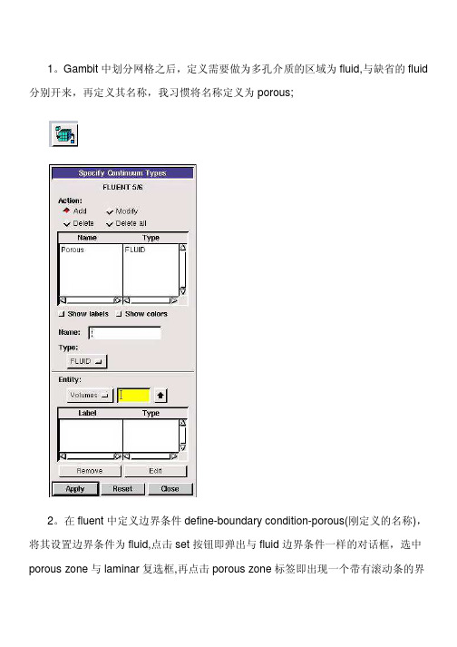
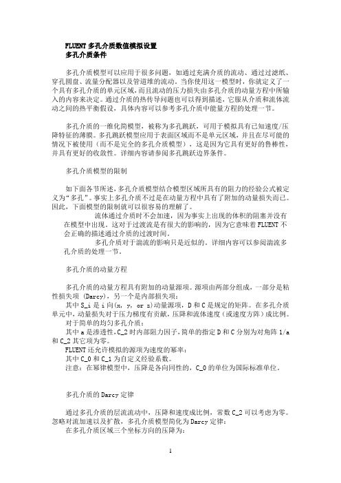
Gambit中划分网格之后,定义需要做为多孔介质的区域为fluid,与缺省的fluid 分别开来,再定义其名称,我习惯将名称定义为porous;2。
在fluent中定义边界条件define-boundary condition-porous(刚定义的名称),将其设置边界条件为fluid,点击set按钮即弹出与fluid边界条件一样的对话框,选中porous zone与laminar复选框,再点击porous zone标签即出现一个带有滚动条的界面;3。
porous zone设置方法:1)定义矢量:二维定义一个矢量,第二个矢量方向不用定义,是与第一个矢量方向正交的;三维定义二个矢量,第三个矢量方向不用定义,是与第一、二个矢量方向正交的;(如何知道矢量的方向:打开grid图,看看X,Y,Z的方向,如果是X向,矢量为1,0,0,同理Y向为0,1,0,Z向为0,0,1,如果所需要的方向与坐标轴正向相反,则定义矢量为负)圆锥坐标与球坐标请参考fluent帮助。
2)定义粘性阻力1/a与内部阻力C2:下面是一个例子:通过实验测得速度和压降进行计算:假设实验所得速度和压降的数值如下:通过多孔介质的为空气,密度为1.225kg/m 3粘度为51.789410µ−=× 。
由上面速度与压降的关系可以绘出一个二次由线。
方程如下:20.28296 4.33539p v v ∇=−简化的动量方程所得二次由线与方程相比较,对应的系数相等,可得210.282962i c v v ρ=4.33539n µα∆=− 设厚度为1m,可以解出20.4621242282c α==−依据些方法计算自己所模拟的模型的粘性阻力和惯性阻力。
3)如果了定义粘性阻力1/a 与内部阻力C2,就不用定义C1与C0,因为这是两种不同的定义方法,C1与C0只在幂率模型中出现,该处保持默认就行了;4)定义孔隙率porousity ,默认值1表示全开放,此值按实验测值填写即可。
FLUENT中多孔介质参数的设置有关问题
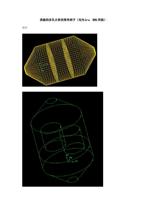
我做的多孔介质的简单例子(均为k-e RNG所做))模型仿真结果多孔介质定义的方法(2008-12-1420:28:12)不知道怎的,这些日子都跟多孔介质干上了1.Define the porous zone.2.Define the porous velocity formulation.(optional)3.Identify the fluid material flowing through the porous medium.4.Enable reactions for the porous zone,if appropriate,and select the reaction mechanism.5.Set the viscous resistance coefficients and the inertial resistance coefficients,and define the direction vectors for which they apply. Alternatively,specify the coefficients for the power-law model.6.Specify the porosity of the porous medium.7.Select the material contained in the porous medium(required only for models that include heat transfer).Note that the specific heat capacity,,for the selected material in the porous zone can only be entered as a constant value.8.Set the volumetric heat generation rate in the solid portion of the porous medium (or any other sources,such as mass or momentum).(optional)9.Set any fixed values for solution variables in the fluid region(optional).10.Suppress the turbulent viscosity in the porous region,if appropriate.11.Specify the rotation axis and/or zone motion,if relevant.fluent中多孔介质porous media设置问题(2008-12-1320:08:07)标签:杂谈分类:CFD计算流体力学经过痛苦的一段经历,终于将局部问题真相大白,为了使保位同仁不再经过我之痛苦,现在将本人多孔介质经验公布如下,希望各位能加精:1。
Fluent计算多孔介质模型资料
广东省深圳市宝安区沙井辛养社区西部工业园 TEL:+86-755-3366-8888 FAX:+86-755-3366-0612Fluent计算多孔介质模型资料这是一个多孔介质例子,进口速度为0.01m/s,组份为液态水和氧气,其中氧气从多孔介质porous jump 渗透过去,如何看氧气在tissue中扩散的。
porous jump的face permeability1 a=e-8 m_2thickness 设为0.0001pressure jump coefficient为默认porous zone设置如下:direction vector 1, 1,viscous resistance 100 eachinertial resistance 100 eachporosity 0.1边界条件设置如下:Ab – wall - defaultBc – wall – defaultBe – porous jump – face permeability 1e-8, porous medium thickness0.0001Cd – outflow rating – 0.5De – wall – defaultDefault interior – interiorDefault interior001 – interiorDefault interior019 – interiorEf – wall - defaultFg – outflow rating – 1Fluid - porous zone - direction vector 1, 1, viscous resistance 100 each,inertial resistance 100 each, porosity 0.1Gh- wall - defaultHi – wall - defaultHk - porous jump same conditions as otherIj – outflow – 0.5Jk – wall – defaultKl – wall – defaultLa – velocity inlet – 0.01 m/s, temperature 300K, 0.5 mass fraction O2 Lfluid – porous zone - direction vector 1, 1, viscous resistance 100 each,inertial resistance 100 each, porosity 0.1Pipefluid – fluid – default (no porous zone)Models – species transport – water and oxygen mixtureVariations – different boundary conditions at top and bottom (outflow, wall ect)注意,其中porous zone在gambit中设置为fluid,在fluent中设置为porous zone边界条件设置如下:Ab – wall - defaultBc – wall – defaultBe – porous jump – face permeability 1e-8, porous medium thickness0.0001Cd – outflow rating – 0.5De – wall – defaultDefault interior – interiorDefault interior001 – interiorDefault interior019 – interiorEf – wall - defaultFg – outflow rating – 1Fluid - porous zone - direction vector 1, 1, viscous resistance 100 each,inertial resistance 100 each, porosity 0.1Gh- wall - defaultHi – wall - defaultHk - porous jump same conditions as otherIj – outflow – 0.5Jk – wall – defaultKl – wall – defaultLa – velocity inlet – 0.01 m/s, temperature 300K, 0.5 mass fraction O2 Lfluid – porous zone - direction vector 1, 1, viscous resistance 100 each,inertial resistance 100 each, porosity 0.1Pipefluid – fluid – default (no porous zone)Models – species transport – water and oxygen mixtureVariations – different boundary conditions at top and bottom (outflow, wall ect) 注意,其中porous zone在gambit中设置为fluid,在fluent中设置为porous zone。
fluent中多孔介质设置问题和算例
经过痛苦的一段经历,终究将局部成绩本相大白,为了使保位同仁不再经过我之痛苦,此刻将本人多孔介质经验公布如下,但愿各位能加精:之杨若古兰创作1.Gambit中划分网格以后,定义须要做为多孔介质的区域为fluid,与缺省的fluid分别开来,再定义其名称,我习气将名称定义为porous;2.在fluent中定义鸿沟条件define-boundary condition-porous(刚定义的名称),将其设置鸿沟条件为fluid,点击set 按钮即弹出与fluid鸿沟条件一样的对话框,选中porous zone与laminar复选框,再点击porous zone标签即出现一个带有滚动条的界面;3.porous zone设置方法:1)定义矢量:二维定义一个矢量,第二个矢量方向不必定义,是与第一个矢量方向正交的;三维定义二个矢量,第三个矢量方向不必定义,是与第一、二个矢量方向正交的;(如何晓得矢量的方向:打开grid图,看看X,Y,Z的方向,如果是X向,矢量为1,0,0,同理Y向为0,1,0,Z向为0,0,1,如果所须要的方向与坐标轴正向相反,则定义矢量为负)圆锥坐标与球坐标请参考fluent帮忙.2)定义粘性阻力1/a与内部阻力C2:请参看本人上一篇博文“终究搞清fluent中多孔粘性阻力与内部阻力的计算方法”,此处不赘述;3)如果了定义粘性阻力1/a与内部阻力C2,就不必定义C1与C0,由于这是两种分歧的定义方法,C1与C0只在幂率模型中出现,该处坚持默认就行了;4)定义孔隙率porousity,默认值1暗示全开放,此值按实验测值填写即可.完了,其他设置与普通k-e或RSM不异.总结一下,与君共享!Tutorial 7. Modeling Flow Through Porous Media IntroductionMany industrial applications involve the modeling of flow through porous media, suchas filters, catalyst beds, and packing. This tutorial illustrates how to set up and solve aproblem involving gas flow through porous media.The industrial problem solved here involves gas flow through acatalytic converter. Catalyticconverters are commonly used to purify emissions from gasoline and diesel enginesby converting environmentally hazardous exhaust emissions to acceptable substances.Examples of such emissions include carbon monoxide (CO), nitrogen oxides (NOx), andunburned hydrocarbon fuels. These exhaust gas emissions are forced through a substrate,which is a ceramic structure coated with a metal catalyst such as platinum or palladium.The nature of the exhaust gas flow is a very important factor in determining the performanceof the catalytic converter. Of particular importance is the pressure gradientand velocity distribution through the substrate. Hence CFD analysis is used to designefficient catalytic converters: by modeling the exhaust gas flow, the pressure drop andthe uniformity of flow through the substrate can be determined. In this tutorial, FLUENTis used to model the flow of nitrogen gas through a catalytic converter geometry, so thatthe flow field structure may be analyzed.This tutorial demonstrates how to do the following:_ Set up a porous zone for the substrate with appropriate resistances._ Calculate a solution for gas flow through the catalytic converterusing the pressurebasedsolver._ Plot pressure and velocity distribution on specified planes of the geometry._ Determine the pressure drop through the substrate and the degree of non-uniformityof flow through cross sections of the geometry using X-Y plots and numerical reports.Problem DescriptionThe catalytic converter modeled here is shown in Figure 7.1. The nitrogen flows inthrough the inlet with a uniform velocity of 22.6 m/s, passes through a ceramic monolithsubstrate with square shaped channels, and then exits through the outlet.While the flow in the inlet and outlet sections is turbulent, the flow through the substrateis laminar and is characterized by inertial and viscous loss coefficients in the flow (X)direction. The substrate is impermeable in other directions, which is modeled using losscoefficients whose values are three orders of magnitude higher than in the X direction.Setup and SolutionStep 1: Grid1. Read the mesh file (catalytic converter.msh).File /Read /Case...2. Check the grid.Grid /CheckFLUENT will perform various checks on the mesh and report the progress in theconsole. Make sure that the minimum volume reported is a positive number.3. Scale the grid.Grid!Scale...(a) Select mm from the Grid Was Created In drop-down list.(b) Click the Change Length Units button.All dimensions will now be shown in millimeters.(c) Click Scale and close the Scale Grid panel.4. Display the mesh.Display /Grid...(a) Make sure that inlet, outlet, substrate-wall, and wall are selected in the Surfacesselection list.(b) Click Display.(c) Rotate the view and zoom in to get the display shown in Figure7.2.(d) Close the Grid Display panel.The hex mesh on the geometry contains a total of 34,580 cells.Step 2: Modelsfine /Models /Solver...2. Select the standard k-εfine/ Models /Viscous...Step 3: Materials1. Add nitrogen to the list of flfine /Materials...(a) Click the Fluent Database... button to open the Fluent Database Materialspanel.i. Select nitrogen (n2) from the list of Fluent Fluid Materials.ii. Click Copy to copy the information for nitrogen to your list of fluid materials.iii. Close the Fluent Database Materials panel.(b) Close the Materials panel.Step 4: Boundary Conditions.Define /Boundary Conditions...1. Set the boundary conditions for the fluid (fluid).(a) Select nitrogen from the Material Name drop-down list.(b) Click OK to close the Fluid panel.2. Set the boundary conditions for the substrate (substrate).(a) Select nitrogen from the Material Name drop-down list.(b) Enable the Porous Zone option to activate the porous zone model.(c) Enable the Laminar Zone option to solve the flow in the porous zone withoutturbulence.(d) Click the Porous Zone tab.i. Make sure that the principal direction vectors are set as shown in e the scroll bar to access the fields that are not initially visible in thepanel.ii. Enter the values in Table 7.2 for the Viscous Resistance and Inertial Resistance.Scroll down to access the fields that are not initially visible in the panel.(e) Click OK to close the Fluid panel.3. Set the velocity and turbulence boundary conditions at the inlet (inlet).(a) Enter 22.6 m/s for the Velocity Magnitude.(b) Select Intensity and Hydraulic Diameter from the Specification Method dropdownlist in the Turbulence group box.(c) Retain the default value of 10% for the Turbulent Intensity.(d) Enter 42 mm for the Hydraulic Diameter.(e) Click OK to close the Velocity Inlet panel.4. Set the boundary conditions at the outlet (outlet).(a) Retain the default setting of 0 for Gauge Pressure.(b) Select Intensity and Hydraulic Diameter from the Specification Method dropdownlist in the Turbulence group box.(c) Enter 5% for the Backflow Turbulent Intensity.(d) Enter 42 mm for the Backflow Hydraulic Diameter.(e) Click OK to close the Pressure Outlet panel.5. Retain the default boundary conditions for the walls (substrate-wall and wall) andclose the Boundary Conditions panel.Step 5: Solution1. Set the solution parameters.Solve /Controls /Solution...(a) Retain the default settings for Under-Relaxation Factors.(b) Select Second Order Upwind from the Momentum drop-down list in the Discretizationgroup box.(c) Click OK to close the Solution Controls panel./Monitors /Residual...(a) Enable Plot in the Options group box.(b) Click OK to close the Residual Monitors panel.3. Enable the plotting of the mass flow rate at the outlet.Solve / Monitors /Surface...(a) Set the Surface Monitors to 1.(b) Enable the Plot and Write options for monitor-1, and click the Define... buttonto open the Define Surface Monitor panel.i. Select Mass Flow Rate from the Report Type drop-down list. ii. Select outlet from the Surfaces selection list.iii. Click OK to close the Define Surface Monitors panel.(c) Click OK to close the Surface Monitors panel.4. Initialize the solution from the inlet.Solve /Initialize /Initialize...(a) Select inlet from the Compute From drop-down list.(b) Click Init and close the Solution Initialization panel.5. Save the case file (catalytic converter.cas).File /Write /Case...6. Run the calculation by requesting 100 iterations.Solve /Iterate...(a) Enter 100 for the Number of Iterations.(b) Click Iterate.The FLUENT calculation will converge in approximately 70 iterations. By thispoint the mass flow rate monitor has attended out, as seen in Figure 7.3.(c) Close the Iterate panel.7. Save the case and data files (catalytic converter.cas and catalytic converter.dat).File /Write /Case & Data...Note: If you choose a file name that already exists in the current folder, FLUENTwill prompt you for confirmation to overwrite the file.Step 6: Post-processing1. Create a surface passing through the centerline for post-processing purposes.Surface/Iso-Surface...(a) Select Grid... and Y-Coordinate from the Surface of Constant drop-down lists.(b) Click Compute to calculate the Min and Max values.(c) Retain the default value of 0 for the Iso-Values.(d) Enter y=0 for the New Surface Name.(e) Click Create.2. Create cross-sectional surfaces at locations on either side of the substrate, as wellas at its center.Surface /Iso-Surface...(a) Select Grid... and X-Coordinate from the Surface of Constant drop-down lists.(b) Click Compute to calculate the Min and Max values.(c) Enter 95 for Iso-Values.(d) Enter x=95 for the New Surface Name.(e) Click Create.(f) In a similar manner, create surfaces named x=130 and x=165 with Iso-Valuesof 130 and 165, respectively. Close the Iso-Surface panel after all the surfaceshave been created.3. Create a line surface for the centerline of the porous media. Surface /Line/Rake...(a) Enter the coordinates of the line under End Points, using the starting coordinateof (95, 0, 0) and an ending coordinate of (165, 0,0), as shown.(b) Enter porous-cl for the New Surface Name.(c) Click Create to create the surface.(d) Close the Line/Rake Surface panel.4. Display the two wall zones (substrate-wall and wall).Display/Grid...(a) Disable the Edges option.(b) Enable the Faces option.(c) Deselect inlet and outlet in the list under Surfaces, and make sure that onlysubstrate-wall and wall are selected.(d) Click Display and close the Grid Display panel.(e) Rotate the view and zoom so that the display is similar to Figure 7.2.5. Set the lighting for the display.Display /Options...(a) Enable the Lights On option in the Lighting Attributes group box.(b) Retain the default selection of Gourand in the Lighting drop-down list.(c) Click Apply and close the Display Options panel.6. Set the transparency parameter for the wall zones (substrate-wall and wall).Display/Scene...(a) Select substrate-wall and wall in the Names selection list.(b) Click the Display... button under Geometry Attributes to openthe DisplayProperties panel.i. Set the Transparency slider to 70.ii. Click Apply and close the Display Properties panel.(c) Click Apply and then close the Scene Description panel.7. Display velocity vectors on the y=0 surface.Display /Vectors...(a) Enable the Draw Grid option.The Grid Display panel will open.i. Make sure that substrate-wall and wall are selected in the list under Surfaces.ii. Click Display and close the Display Grid panel.(b) Enter 5 for the Scale.(c) Set Skip to 1.(d) Select y=0 from the Surfaces selection list.(e) Click Display and close the Vectors panel.The flow pattern shows that the flow enters the catalytic converter as a jet, withrecirculation on either side of the jet. As it passes through the porous substrate, itdecelerates and straightens out, and exhibits a more uniform velocity distribution.This allows the metal catalyst present in the substrate to be more effective.Figure 7.4: Velocity Vectors on the y=0 Plane8. Display filled contours of static pressure on the y=0 plane. Display /Contours...(a) Enable the Filled option.(b) Enable the Draw Grid option to open the Display Grid panel.i. Make sure that substrate-wall and wall are selected in the list under Surfaces.ii. Click Display and close the Display Grid panel.(c) Make sure that Pressure... and Static Pressure are selected from the Contoursof drop-down lists.(d) Select y=0 from the Surfaces selection list.(e) Click Display and close the Contours panel.Figure 7.5: Contours of the Static Pressure on the y=0 planeThe pressure changes rapidly in the middle section, where the fluid velocity changesas it passes through the porous substrate. The pressure drop can be high, due to theinertial and viscous resistance of the porous media. Determining this pressure dropis a goal of CFD analysis. In the next step, you will learn how to plot the pressuredrop along the centerline of the substrate.9. Plot the static pressure across the line surface porous-cl.Plot /XY Plot...(a) Make sure that the Pressure... and Static Pressure are selectedfrom the Y AxisFunction drop-down lists.(b) Select porous-cl from the Surfaces selection list.(c) Click Plot and close the Solution XY Plot panel.Figure 7.6: Plot of the Static Pressure on the porous-cl Line SurfaceIn Figure 7.6, the pressure drop across the porous substrate can be seen to beroughly 300 Pa.10. Display filled contours of the velocity in the X direction on the x=95, x=130 andx=165 surfaces.Display /Contours...(a) Disable the Global Range option.(b) Select Velocity... and X Velocity from the Contours of drop-down lists.(c) Select x=130, x=165, and x=95 from the Surfaces selection list, and deselecty=0.(d) Click Display and close the Contours panel.The velocity profile becomes more uniform as the fluid passes through the porousmedia. The velocity is very high at the center (the area in red) just before thenitrogen enters the substrate and then decreases as it passes through and exits thesubstrate. The area in green, which corresponds to a moderate velocity, increasesin extent.Figure 7.7: Contours of the X Velocity on the x=95,x=130, and x=165 Surfaces11. Use numerical reports to determine the average, minimum, and maximum of thevelocity distribution before and after the porous substrate.Report /Surface Integrals...(a) Select Mass-Weighted Average from the Report Type drop-down list.(b) Select Velocity and X Velocity from the Field Variable drop-down lists.(c) Select x=165 and x=95 from the Surfaces selection list.(d) Click Compute.(e) Select Facet Minimum from the Report Type drop-down list and click Computeagain.(f) Select Facet Maximum from the Report Type drop-down list and click Computeagain.(g) Close the Surface Integrals panel.The numerical report of average, maximum and minimum velocity can be seen inthe main FLUENT console, as shown in the following example:The spread between the average, maximum, and minimum values for X velocitygives the degree to which the velocity distribution isnon-uniform. You can also usethese numbers to calculate the velocity ratio (i.e., the maximum velocity divided bythe mean velocity) and the space velocity (i.e., the product of the mean velocity andthe substrate length).Custom field functions and UDFs can be also used to calculate more complex measuresof non-uniformity, such as the standard deviation and the gamma uniformityindex.SummaryIn this tutorial, you learned how to set up and solve a problem involving gas flow throughporous media in FLUENT. You also learned how to perform appropriate post-processingto investigate the flow field, determine the pressure drop across the porous media andnon-uniformity of the velocity distribution as the fluid goes through the porous media.Further ImprovementsThis tutorial guides you through the steps to reach an initial solution. You may be ableto obtain a more accurate solution by using an appropriate higher-order discretizationscheme and by adapting the grid. Grid adaption can also ensure that the solution isindependent of the grid. These steps are demonstrated in Tutorial 1.。
fluent中多孔介质设置问题和算例
经过痛苦的一段经历;终于将局部问题真相大白;为了使保位同仁不再经过我之痛苦;现在将本人多孔介质经验公布如下;希望各位能加精:1..Gambit中划分网格之后;定义需要做为多孔介质的区域为fluid;与缺省的fluid分别开来;再定义其名称;我习惯将名称定义为porous;2..在fluent中定义边界条件define-boundary condition-porous刚定义的名称;将其设置边界条件为fluid;点击set按钮即弹出与fluid边界条件一样的对话框;选中porous zone 与laminar复选框;再点击porous zone标签即出现一个带有滚动条的界面;3..porous zone设置方法:1定义矢量:二维定义一个矢量;第二个矢量方向不用定义;是与第一个矢量方向正交的;三维定义二个矢量;第三个矢量方向不用定义;是与第一、二个矢量方向正交的;如何知道矢量的方向:打开grid图;看看X;Y;Z的方向;如果是X向;矢量为1;0;0;同理Y 向为0;1;0;Z向为0;0;1;如果所需要的方向与坐标轴正向相反;则定义矢量为负圆锥坐标与球坐标请参考fluent帮助..2定义粘性阻力1/a与内部阻力C2:请参看本人上一篇博文“终于搞清fluent中多孔粘性阻力与内部阻力的计算方法”;此处不赘述;3如果了定义粘性阻力1/a与内部阻力C2;就不用定义C1与C0;因为这是两种不同的定义方法;C1与C0只在幂率模型中出现;该处保持默认就行了;4定义孔隙率porousity;默认值1表示全开放;此值按实验测值填写即可..完了;其他设置与普通k-e或RSM相同..总结一下;与君共享Tutorial 7. Modeling Flow Through Porous MediaIntroductionMany industrial applications involve the modeling of flow through porous media; such as filters; catalyst beds; and packing. This tutorial illustrates how to set up and solve a problem involving gas flow through porous media.The industrial problem solved here involves gas flow through a catalytic converter. Catalytic converters are commonly used to purify emissions from gasoline and diesel engines by converting environmentally hazardous exhaust emissions to acceptable substances.Examples of such emissions include carbon monoxide CO; nitrogen oxides NOx; and unburned hydrocarbon fuels. These exhaust gas emissions are forced through a substrate; which is a ceramic structure coated with a metal catalyst such as platinum or palladium.The nature of the exhaust gas flow is a very important factor in determining the performance of the catalytic converter. Of particular importance is the pressure gradient and velocity distribution through the substrate. Hence CFD analysis is used to design efficient catalytic converters: by modeling the exhaust gas flow; the pressure drop and the uniformity of flow through the substrate can be determined. In this tutorial; FLUENT is used to model the flow of nitrogen gas through a catalytic converter geometry; so that the flow field structure may be analyzed.This tutorial demonstrates how to do the following:_ Set up a porous zone for the substrate with appropriate resistances._ Calculate a solution for gas flow through the catalytic converter using the pressure based solver. _ Plot pressure and velocity distribution on specified planes of the geometry._ Determine the pressure drop through the substrate and the degree of non-uniformity of flow through cross sections of the geometry using X-Y plots and numerical reports.Problem DescriptionThe catalytic converter modeled here is shown in Figure 7.1. The nitrogen flows in through the inlet with a uniform velocity of 22.6 m/s; passes through a ceramic monolith substrate with square shaped channels; and then exits through the outlet.While the flow in the inlet and outlet sections is turbulent; the flow through the substrate is laminar and is characterized by inertial and viscous loss coefficients in the flow X direction. The substrate is impermeable in other directions; which is modeled using loss coefficients whose values are three orders of magnitude higher than in the X direction.Setup and SolutionStep 1: Grid1. Read the mesh file catalytic converter.msh.File /Read /Case...2. Check the grid. Grid /CheckFLUENT will perform various checks on the mesh and report the progress in the console. Make sure that the minimum volume reported is a positive number.3. Scale the grid.Grid Scale...a Select mm from the Grid Was Created In drop-down list.b Click the Change Length Units button. All dimensions will now be shown in millimeters.c Click Scale and close the Scale Grid panel.4. Display the mesh. Display /Grid...a Make sure that inlet; outlet; substrate-wall; and wall are selected in the Surfaces selection list.b Click Display.c Rotate the view and zoom in to get the display shown in Figure 7.2.d Close the Grid Display panel.The hex mesh on the geometry contains a total of 34;580 cells.Step 2: Models1. Retain the default solver settings. Define /Models /Solver...2. Select the standard k-ε turbulence model. Define/ Models /Viscous...Step 3: Materials1. Add nitrogen to the list of fluid materials by copying it from the Fluent Database for materials.Define /Materials...a Click the Fluent Database... button to open the Fluent Database Materials panel.i. Select nitrogen n2 from the list of Fluent Fluid Materials.ii. Click Copy to copy the information for nitrogen to your list of fluid materials. iii. Close the Fluent Database Materials panel.b Close the Materials panel.Step 4: Boundary Conditions. Define /Boundary Conditions...1. Set the boundary conditions for the fluid fluid.a Select nitrogen from the Material Name drop-down list.b Click OK to close the Fluid panel.2. Set the boundary conditions for the substrate substrate.a Select nitrogen from the Material Name drop-down list.b Enable the Porous Zone option to activate the porous zone model.c Enable the Laminar Zone option to solve the flow in the porous zone without turbulence.d Click the Porous Zone tab.i. Make sure that the principal direction vectors are set as shown in Table7.1. Use the scroll bar to access the fields that are not initially visible in the panel.ii. Enter the values in Table 7.2 for the Viscous Resistance and Inertial Resistance. Scroll down to access the fields that are not initially visible in the panel.e Click OK to close the Fluid panel.3. Set the velocity and turbulence boundary conditions at the inlet inlet.a Enter 22.6 m/s for the Velocity Magnitude.b Select Intensity and Hydraulic Diameter from the Specification Method dropdown list in the Turbulence group box.c Retain the default value of 10% for the Turbulent Intensity.d Enter 42 mm for the Hydraulic Diameter.e Click OK to close the Velocity Inlet panel.4. Set the boundary conditions at the outlet outlet.a Retain the default setting of 0 for Gauge Pressure.b Select Intensity and Hydraulic Diameter from the Specification Method dropdown list in the Turbulence group box.c Enter 5% for the Backflow Turbulent Intensity.d Enter 42 mm for the Backflow Hydraulic Diameter.e Click OK to close the Pressure Outlet panel.5. Retain the default boundary conditions for the walls substrate-wall and wall and close the Boundary Conditions panel.Step 5: Solution1. Set the solution parameters. Solve /Controls /Solution...a Retain the default settings for Under-Relaxation Factors.b Select Second Order Upwind from the Momentum drop-down list in the Discretization group box.c Click OK to close the Solution Controls panel.2. Enable the plotting of residuals during the calculation. Solve/Monitors /Residual...a Enable Plot in the Options group box.b Click OK to close the Residual Monitors panel.3. Enable the plotting of the mass flow rate at the outlet.Solve / Monitors /Surface...a Set the Surface Monitors to 1.b Enable the Plot and Write options for monitor-1; and click the Define... button to open the Define Surface Monitor panel.i. Select Mass Flow Rate from the Report Type drop-down list.ii. Select outlet from the Surfaces selection list.iii. Click OK to close the Define Surface Monitors panel.c Click OK to close the Surface Monitors panel.4. Initialize the solution from the inlet. Solve /Initialize /Initialize...a Select inlet from the Compute From drop-down list.b Click Init and close the Solution Initialization panel.5. Save the case file catalytic converter.cas. File /Write /Case...6. Run the calculation by requesting 100 iterations. Solve /Iterate...a Enter 100 for the Number of Iterations.b Click Iterate.The FLUENT calculation will converge in approximately 70 iterations. By this point the mass flow rate monitor has attended out; as seen in Figure 7.3.c Close the Iterate panel.7. Save the case and data files catalytic converter.cas and catalytic converter.dat.File /Write /Case & Data...Note: If you choose a file name that already exists in the current folder; FLUENTwill prompt you for confirmation to overwrite the file.Step 6: Post-processing1. Create a surface passing through the centerline for post-processing purposes.Surface/Iso-Surface...a Select Grid... and Y-Coordinate from the Surface of Constant drop-down lists.b Click Compute to calculate the Min and Max values.c Retain the default value of 0 for the Iso-Values.d Enter y=0 for the New Surface Name.e Click Create.2. Create cross-sectional surfaces at locations on either side of the substrate; as well as at its center.Surface /Iso-Surface...a Select Grid... and X-Coordinate from the Surface of Constant drop-down lists.b Click Compute to calculate the Min and Max values.c Enter 95 for Iso-Values.d Enter x=95 for the New Surface Name.e Click Create.f In a similar manner; create surfaces named x=130 and x=165 with Iso-Values of 130 and 165; respectively. Close the Iso-Surface panel after all the surfaces have been created.3. Create a line surface for the centerline of the porous media.Surface /Line/Rake...a Enter the coordinates of the line under End Points; using the starting coordinate of 95; 0; 0 and an ending coordinate of 165; 0; 0; as shown.b Enter porous-cl for the New Surface Name.c Click Create to create the surface.d Close the Line/Rake Surface panel.4. Display the two wall zones substrate-wall and wall. Display /Grid...a Disable the Edges option.b Enable the Faces option.c Deselect inlet and outlet in the list under Surfaces; and make sure that only substrate-wall and wall are selected.d Click Display and close the Grid Display panel.e Rotate the view and zoom so that the display is similar to Figure 7.2.5. Set the lighting for the display. Display /Options...a Enable the Lights On option in the Lighting Attributes group box.b Retain the default selection of Gourand in the Lighting drop-down list.c Click Apply and close the Display Options panel.6. Set the transparency parameter for the wall zones substrate-wall and wall.Display/Scene...a Select substrate-wall and wall in the Names selection list.b Click the Display... button under Geometry Attributes to open the Display Properties panel.i. Set the Transparency slider to 70.ii. Click Apply and close the Display Properties panel.c Click Apply and then close the Scene Description panel.7. Display velocity vectors on the y=0 surface.Display /Vectors...a Enable the Draw Grid option. The Grid Display panel will open.i. Make sure that substrate-wall and wall are selected in the list under Surfaces.ii. Click Display and close the Display Grid panel.b Enter 5 for the Scale.c Set Skip to 1.d Select y=0 from the Surfaces selection list.e Click Display and close the Vectors panel.The flow pattern shows that the flow enters the catalytic converter as a jet; with recirculation on either side of the jet. As it passes through the porous substrate; it decelerates and straightens out; and exhibits a more uniform velocity distribution.This allows the metal catalyst present in the substrate to be more effective.Figure 7.4: Velocity Vectors on the y=0 Plane8. Display filled contours of static pressure on the y=0 plane.Display /Contours...a Enable the Filled option.b Enable the Draw Grid option to open the Display Grid panel.i. Make sure that substrate-wall and wall are selected in the list under Surfaces.ii. Click Display and close the Display Grid panel.c Make sure that Pressure... and Static Pressure are selected from the Contours of drop-down lists.d Select y=0 from the Surfaces selection list.e Click Display and close the Contours panel.Figure 7.5: Contours of the Static Pressure on the y=0 planeThe pressure changes rapidly in the middle section; where the fluid velocity changes as it passes through the porous substrate. The pressure drop can be high; due to the inertial and viscous resistance of the porous media. Determining this pressure drop is a goal of CFD analysis. In the next step; you will learn how to plot the pressure drop along the centerline of the substrate.9. Plot the static pressure across the line surface porous-cl.Plot /XY Plot...a Make sure that the Pressure... and Static Pressure are selected from the Y Axis Function drop-down lists.b Select porous-cl from the Surfaces selection list.c Click Plot and close the Solution XY Plot panel.Figure 7.6: Plot of the Static Pressure on the porous-cl Line SurfaceIn Figure 7.6; the pressure drop across the porous substrate can be seen to be roughly 300 Pa.10. Display filled contours of the velocity in the X direction on the x=95; x=130 and x=165 surfaces.Display /Contours...a Disable the Global Range option.b Select Velocity... and X Velocity from the Contours of drop-down lists.c Select x=130; x=165; and x=95 from the Surfaces selection list; and deselect y=0.d Click Display and close the Contours panel.The velocity profile becomes more uniform as the fluid passes through the porous media. The velocity is very high at the center the area in red just before the nitrogen enters the substrate and then decreases as it passes through and exits the substrate. The area in green; which corresponds to a moderate velocity; increases in extent.Figure 7.7: Contours of the X Velocity on the x=95; x=130; and x=165 Surfaces11. Use numerical reports to determine the average; minimum; and maximum of the velocity distribution before and after the porous substrate.Report /Surface Integrals...a Select Mass-Weighted Average from the Report Type drop-down list.b Select Velocity and X Velocity from the Field Variable drop-down lists.c Select x=165 and x=95 from the Surfaces selection list.d Click Compute.e Select Facet Minimum from the Report Type drop-down list and click Compute again.f Select Facet Maximum from the Report Type drop-down list and click Compute again.g Close the Surface Integrals panel.The numerical report of average; maximum and minimum velocity can be seen in the main FLUENT console; as shown in the following example:The spread between the average; maximum; and minimum values for X velocity gives the degree to which the velocity distribution is non-uniform. You can also use these numbers to calculate the velocity ratio i.e.; the maximum velocity divided by the mean velocity and the space velocity i.e.; the product of the mean velocity and the substrate length.Custom field functions and UDFs can be also used to calculate more complex measures ofnon-uniformity; such as the standard deviation and the gamma uniformity index.SummaryIn this tutorial; you learned how to set up and solve a problem involving gas flow through porous media in FLUENT. You also learned how to perform appropriate post-processing to investigate the flow field; determine the pressure drop across the porous media and non-uniformity of the velocity distribution as the fluid goes through the porous media.Further ImprovementsThis tutorial guides you through the steps to reach an initial solution. You may be able to obtain a more accurate solution by using an appropriate higher-order discretization scheme and by adapting the grid. Grid adaption can also ensure that the solution is independent of the grid. These steps aredemonstrated in Tutorial 1.。
FLUENT多孔介质数值模拟设置
FLUENT多孔介质数值模拟设置多孔介质条件多孔介质模型可以应用于很多问题,如通过充满介质的流动、通过过滤纸、穿孔圆盘、流量分配器以及管道堆的流动。
当你使用这一模型时,你就定义了一个具有多孔介质的单元区域,而且流动的压力损失由多孔介质的动量方程中所输入的内容来决定。
通过介质的热传导问题也可以得到描述,它服从介质和流体流动之间的热平衡假设,具体内容可以参考多孔介质中能量方程的处理一节。
多孔介质的一维化简模型,被称为多孔跳跃,可用于模拟具有已知速度/压降特征的薄膜。
多孔跳跃模型应用于表面区域而不是单元区域,并且在尽可能的情况下被使用(而不是完全的多孔介质模型),这是因为它具有更好的鲁棒性,并具有更好的收敛性。
详细内容请参阅多孔跳跃边界条件。
多孔介质模型的限制如下面各节所述,多孔介质模型结合模型区域所具有的阻力的经验公式被定义为“多孔”。
事实上多孔介质不过是在动量方程中具有了附加的动量损失而已。
因此,下面模型的限制就可以很容易的理解了。
流体通过介质时不会加速,因为事实上出现的体积的阻塞并没有在模型中出现。
这对于过渡流是有很大的影响的,因为它意味着FLUENT不会正确的描述通过介质的过渡时间。
多孔介质对于湍流的影响只是近似的。
详细内容可以参阅湍流多孔介质的处理一节。
多孔介质的动量方程多孔介质的动量方程具有附加的动量源项。
源项由两部分组成,一部分是粘性损失项 (Darcy),另一个是内部损失项:其中S_i是i向(x, y, or z)动量源项,D和C是规定的矩阵。
在多孔介质单元中,动量损失对于压力梯度有贡献,压降和流体速度(或速度方阵)成比例。
对于简单的均匀多孔介质:其中a是渗透性,C_2时内部阻力因子,简单的指定D和C分别为对角阵1/a 和C_2其它项为零。
FLUENT还允许模拟的源项为速度的幂率:其中C_0和C_1为自定义经验系数。
注意:在幂律模型中,压降是各向同性的,C_0的单位为国际标准单位。
多孔介质的Darcy定律通过多孔介质的层流流动中,压降和速度成比例,常数C_2可以考虑为零。
- 1、下载文档前请自行甄别文档内容的完整性,平台不提供额外的编辑、内容补充、找答案等附加服务。
- 2、"仅部分预览"的文档,不可在线预览部分如存在完整性等问题,可反馈申请退款(可完整预览的文档不适用该条件!)。
- 3、如文档侵犯您的权益,请联系客服反馈,我们会尽快为您处理(人工客服工作时间:9:00-18:30)。
FLUENT多孔介质数值模拟设置多孔介质条件多孔介质模型可以应用于很多问题,如通过充满介质的流动、通过过滤纸、穿孔圆盘、流量分配器以及管道堆的流动。
当你使用这一模型时,你就定义了一个具有多孔介质的单元区域,而且流动的压力损失由多孔介质的动量方程中所输入的内容来决定。
通过介质的热传导问题也可以得到描述,它服从介质和流体流动之间的热平衡假设,具体内容可以参考多孔介质中能量方程的处理一节。
多孔介质的一维化简模型,被称为多孔跳跃,可用于模拟具有已知速度/压降特征的薄膜。
多孔跳跃模型应用于表面区域而不是单元区域,并且在尽可能的情况下被使用(而不是完全的多孔介质模型),这是因为它具有更好的鲁棒性,并具有更好的收敛性。
详细内容请参阅多孔跳跃边界条件。
多孔介质模型的限制如下面各节所述,多孔介质模型结合模型区域所具有的阻力的经验公式被定义为“多孔”。
事实上多孔介质不过是在动量方程中具有了附加的动量损失而已。
因此,下面模型的限制就可以很容易的理解了。
流体通过介质时不会加速,因为事实上出现的体积的阻塞并没有在模型中出现。
这对于过渡流是有很大的影响的,因为它意味着FLUENT不会正确的描述通过介质的过渡时间。
多孔介质对于湍流的影响只是近似的。
详细内容可以参阅湍流多孔介质的处理一节。
多孔介质的动量方程多孔介质的动量方程具有附加的动量源项。
源项由两部分组成,一部分是粘性损失项 (Darcy),另一个是内部损失项:其中S_i是i向(x, y, or z)动量源项,D和C是规定的矩阵。
在多孔介质单元中,动量损失对于压力梯度有贡献,压降和流体速度(或速度方阵)成比例。
对于简单的均匀多孔介质:其中a是渗透性,C_2时内部阻力因子,简单的指定D和C分别为对角阵1/a 和C_2其它项为零。
FLUENT还允许模拟的源项为速度的幂率:其中C_0和C_1为自定义经验系数。
注意:在幂律模型中,压降是各向同性的,C_0的单位为国际标准单位。
多孔介质的Darcy定律通过多孔介质的层流流动中,压降和速度成比例,常数C_2可以考虑为零。
忽略对流加速以及扩散,多孔介质模型简化为Darcy定律:在多孔介质区域三个坐标方向的压降为:其中为多孔介质动量方程1中矩阵D的元素v为三个方向上的分速度,Djn_x、 D n_y、以及D n_z为三个方向上的介质厚度。
在这里介质厚度其实就是模型区域内的多孔区域的厚度。
因此如果模型的厚度和实际厚度不同,你必须调节1/a_ij的输入。
.多孔介质的内部损失在高速流动中,多孔介质动量方程1中的常数C_2提供了多孔介质内部损失的矫正。
这一常数可以看成沿着流动方向每一单位长度的损失系数,因此允许压降指定为动压头的函数。
如果你模拟的是穿孔板或者管道堆,有时你可以消除渗透项而只是用内部损失项,从而得到下面的多孔介质简化方程:写成坐标形式为:多孔介质中能量方程的处理对于多孔介质流动,FLUENT仍然解标准能量输运方程,只是修改了传导流量和过度项。
在多孔介质中,传导流量使用有效传导系数,过渡项包括了介质固体区域的热惯量:其中:h_f=流体的焓h_s=固体介质的焓f=介质的多孔性k_eff=介质的有效热传导系数S^h_f=流体焓的源项S^h_s=固体焓的源项多孔介质的有效传导率多孔区域的有效热传导率k_eff是由流体的热传导率和固体的热传导率的体积平均值计算得到:其中:f=介质的多孔性k_f=流体状态热传导率(包括湍流的贡献k_t)k_s=固体介质热传导率如果得不到简单的体积平均,可能是因为介质几何外形的影响。
有效传导率可以用自定义函数来计算。
然而,在所有的算例中,有效传导率被看成介质的各向同性性质。
多孔介质中的湍流处理在多孔介质中,默认的情况下FLUENT会解湍流量的标准守恒防城。
因此,在这种默认的方法中,介质中的湍流被这样处理:固体介质对湍流的生成和耗散速度没有影响。
如果介质的渗透性足够大,而且介质的几何尺度和湍流涡的尺度没有相互作用,这样的假设是合情合理的。
但是在其它的一些例子中,你会压制了介质中湍流的影响。
如果你使用k-e模型或者Spalart-Allmaras模型,你如果设定湍流对粘性的贡献m_t为零,你可能会压制了湍流对介质的影响。
当你选择这一选项时,FLUENT会将入口湍流的性质传输到介质中,但是它对流动混合和动量的影响被忽略了。
除此之外,在介质中湍流的生成也被设定为零。
要实现这一解策略,请在流体面板中打开层流选项。
激活这个选项就意味着多孔介质中的m_t为零,湍流的生成也为零。
如果去掉该选项(默认)则意味着多孔介质中的湍流会像大体积流体流动一样被计算。
概述模拟多孔介质流动时,对于问题设定需要的附加输入如下:1. 定义多孔区域2. 确定流过多孔区域的流体材料3. 设定粘性系数(多孔介质动量方程3中的1/a_ij)以及内部阻力系数(多孔介质动量方程3中的C_2_ij),并定义应用它们的方向矢量。
幂率模型的系数也可以选择指定。
4. 定义多孔介质包含的材料属性和多孔性5. 设定多孔区域的固体部分的体积热生成速度(或任何其它源项,如质量、动量)(此项可选)。
6. 如果合适的话,限制多孔区域的湍流粘性。
7. 如果相关的话,指定旋转轴和/或区域运动。
在定义粘性和内部阻力系数中描述了决定阻力系数和/或渗透性的方法。
如果你使用多孔动量源项的幂律近似,你需要输入多孔介质动量方程5中的C_0和C_1来取代阻力系数和流动方向。
在流体面板中(下图)你需要设定多孔介质的所有参数,该面板是从边界条件菜单中打开的(详细内容请参阅边界条件的设定一节)Figure 1:多孔区域的流体面板定义多孔区域正如定义边界条件概述中所提到的,多孔区域是作为特定类型的流体区域来模拟的。
亚表明流体区域是多孔区域,请在流体面板中激活多孔区域选项。
面板会自动扩展到多孔介质输入状态。
定义穿越多孔介质的流体在材料名字下拉菜单中选择适当的流体就可以定义通过多孔介质的流体了。
如果你模拟组分输运或者多相流,流体面板中就不会出现材料名字下拉菜单了。
对于组分计算,所有流体和/或多孔区域的混合材料就是你在组分模型面板中指定的材料。
对于多相流模型,所有流体和/或多孔区域的混合材料就是你在多相流模型面板中指定的材料。
定义粘性和内部阻力系数粘性和内部阻力系数以相同的方式定义。
使用笛卡尔坐标系定义系数的基本方法是在二维问题中定义一个方向矢量,在三维问题中定义两个方向矢量,然后在每个方向上指定粘性和/或阻力系数。
在二维问题中第二个方向没有明确定义,它是垂直于指定的方向矢量和z向矢量所在的平面的。
在三维问题中,第三个方向矢量是垂直于所指定的两个方向矢量所在平面的。
对于三维问题,第二个方向矢量必须垂直于第一个方向矢量。
如果第二个方向矢量指定失败,解算器会确保它们垂直而忽略在第一个方向上的第二个矢量的任何分量。
所以你应该确保第一个方向指定正确。
在三维问题中也可能会使用圆锥(或圆柱)坐标系来定义系数,具体如下:定义阻力系数的过程如下:1. 定义方向矢量。
使用笛卡尔坐标系,简单指定方向1矢量,如果是三维问题,指定方向2矢量。
每一个方向都应该是从(0,0)或者(0,0,0)到指定的(X,Y)或(X,Y,Z)矢量。
(如果方向不正确请按上面的方法解决)对于有些问题,多孔介质的主轴和区域的坐标轴不在一条直线上,你不必知道多孔介质先前的方向矢量。
在这种情况下,三维中的平面工具或者二维中的线工具可以帮你确定这些方向矢量。
1. 捕捉"Snap"平面工具(或者线工具)到多孔区域的边界。
(请遵循使用面工具和线工具中的说明,它在已存在的表面上为工具初始化了位置)。
2. 适当的旋转坐标轴直到它们和多孔介质区域成一条线。
3. 当成一条线之后,在流体面板中点击从平面工具更新或者从线工具更新按钮。
FLUENT会自动将方向1矢量指向为工具的红(三维)或绿(二维)箭头所指的方向。
要使用圆锥坐标系(比方说环状、锥状顾虑单元),请遵循下面步骤(这一选项只用于三维问题):1. 打开圆锥选项2. 指定圆锥轴矢量和在锥轴上的点。
圆锥轴矢量的方向将会是从(0,0,0)到指定的(X,Y,Z)方向的矢量。
FLUENT将会使用圆锥轴上的点将阻力转换到笛卡尔坐标系。
3. 设定锥半角(锥轴和锥表面之间的角度,如下图),使用柱坐标系,锥半角为0.Figure 1:锥半角对于有些问题,锥形过滤单元的主轴和区域的坐标轴不在一条直线上,你不必知道锥轴先前的方向矢量以及锥轴上的点。
在这种情况下,三维中的平面工具或者二维中的线工具可以帮你确定这些方向矢量。
一种方法如下:1. 在点击捕捉到区域按钮之前,你可以在下拉菜单中选择垂直于锥轴矢量的轴过滤单元的边界区域。
2. 点击捕捉到区域按钮,FLUENT会自动将平面工具捕捉到边界。
它也会设定锥轴矢量和锥轴上的点(需注意的是你还要自己设定锥半角)。
另一种方法为:1. 捕捉"Snap"平面工具到多孔区域的边界。
(请遵循使用面工具和线工具中的说明,它在已存在的表面上为工具初始化了位置)。
2. 旋转和平移工具坐标轴,直到工具的红箭头指向锥的轴向。
工具的起点在轴上。
3. 当轴和工具的起点成一条线时,在流体面板中点击从平面工具更新按钮。
FLUENT会自动设定轴向矢量以及在轴上的点(注意:你还是要自己设定锥的半角)。
2. 在粘性阻力中指定每个方向的粘性阻力系数1/a,在内部阻力中指定每一个方向上的内部阻力系数C_2(你可能需要将滚动条向下滚动来查看这些输入)。
如果你使用锥指定方法,方向1为锥轴方向,方向2为垂直于锥表面(对于圆柱就是径向)方向,方向3圆周(q)方向。
在三维问题中可能有三种可能的系数,在二维问题中有两种:在各向同性算例中,所有方向上的阻力系数都是相等的(如海绵)。
在各向同性算例中你必须将每个方向上的阻力系数设定为相等。
在三维问题中只有两个方向上的系数相等,第三个方向上的阻力系数和前两个不等,或者在二维问题中两个方向上的系数不等,你必须准确的指定每一个方向上的系数。
例如,如果你得多孔区域是由具有小洞的细管组成,细管平行于流动方向,流动会很容易的通过细管,但是流动在其它两个方向上(通过小洞)会很小。
如果你有一个平的盘子垂直于流动方向,流动根本就不会穿过它而只在其它两个方向上。
在三维问题中还有一种可能就是三个系数各不相同。
例如,如果多孔区域是由不规则间隔的物体(如针脚)组成的平面,那么阻碍物之间的流动在每个方向上都不同。
此时你就需要在每个方向上指定不同的系数(请注意指定各向同性系数时,多孔介质的解策略的注解)。
推导粘性和内部损失系数的方法在定义粘性和内部阻力系数一节中介绍。
当你使用多孔介质模型时,你必须记住FLUENT中的多孔单元是100%打开的,而且你所指定1/a_ij和/或C_2_ij的值必须是基于这个假设的。