Distributed representations hinton1984
hinton 知识蒸馏 kl散度损失函数

hinton 知识蒸馏 kl散度损失函数知识蒸馏是指将一个大型深度神经网络的知识迁移到一个较小的网络中。
这不仅可以使网络更加轻便,还可以提高推理速度和精度,因为较小的网络学习到了更精华的信息。
Hinton是最早推广知识蒸馏的人之一。
他提出的知识蒸馏方法是基于一种特定的模型蒸馏,其核心思想是使用一个小模型去模仿大模型的预测行为。
本文将围绕Hinton知识蒸馏KL散度损失函数进行讲解。
第一步:问题引入当一个大型的深度神经网络完成训练后,我们可以将这个网络视为“老师”模型,它拥有丰富的知识。
但是,由于其庞大的模型和参数数量,它过于复杂,不适合在嵌入式系统、移动设备和低端硬件上运行和部署。
那么,我们怎样才能让小型网络具备大型网络同样的精度呢?第二步:基本原理知识蒸馏的基本思想是将大型网络的丰富知识蒸馏到一个小型网络中,以达到精度相同甚至更高的效果。
在知识蒸馏中,我们需要使用某些方法将老师网络的知识转移到学生网络中。
将软性目标函数添加到学生网络中,来抓住大型网络的行为,并在学生网络的损失函数中添加额外的项,以帮助学生网络更好地学习。
第三步:KL散度KL散度自然是知识蒸馏损失函数中很重要的一部分。
在知识蒸馏损失函数中,KL散度是一个重要的元素之一,它用于量化大型网络和小型网络之间的差异。
KL散度可描述两个概率分布之间的差异,是两个概率分布之间的非对称度量。
第四步:确定损失函数Hinton提出的知识蒸馏KL散度损失函数的公式如下:$KD(P||Q)=\sum_{x}P(x)\log\frac{P(x)}{Q(x)}$其中,P(x)代表老师网络的输出,Q(x)代表学生网络的输出,x代表输出的标签或类别。
此时,KL散度可以用于计算输出分布的差异。
参数T是一个温度参数,它作为一个类似于softmax函数的称为“软化”的激活函数的分母的标准偏差来控制输出分布的熵。
T越大,输出的分布越“平坦”,T越小,输出的分布越“峰形”。
深度学习研究综述
的第 i个神经元被激活函数作用之前的值,Wlji是第 l层的
第 j个神经元与第 l+1层的第 i个神经元之间的权重,bli
是偏置,f(·)是非线性激活函数,常见的有径向基函数、
ReLU、PReLU、Tanh、Sigmoid等.
如果采用均方误差(meansquarederror),则损失函数为
∑ J=
Keywords
deeplearning; neuralnetwork; machinelearning; artificialintelligence; convolutionalneuralnetwork; recurrentneuralnetwork
0 引言
2016年 3月,“人工智能”一词被写入中国“十三五” 规划纲要,2016年 10月美国政府发布《美国国家人工智能 研究与发展 战 略 规 划 》文 件.Google、大对人 工智能的投入.各类人工智能创业公司层出不穷,各种人 工智能应用逐渐改变人类的生活.深度学习是目前人工智 能的重点研究领域之一,应用于人工智能的众多领域,包 括语音处理、计算机视觉、自然语言处理等.
适合处理空间数据,在计算机视觉领域应用广泛.一维卷
积神经网络也被称 为 时 间 延 迟 神 经 网 络 (timedelayneural network),可以用来处理一维数据.CNN的设计思想受到 了视觉神经 科 学 的 启 发,主 要 由 卷 积 层 (convolutionallay er)和池化层(poolinglayer)组成.卷积层能够保持图像的 空间连续性,能将图像的局部特征提取出来.池化层可以 采用最大 池 化 (maxpooling)或 平 均 池 化 (meanpooling), 池化层能降低中间隐藏层的维度,减少接下来各层的运算 量,并提供了旋转不变性.卷积与池化操作示意图如图 3 所示,图中采用 3×3的卷积核和 2×2的 pooling.
机器学习领域的知名人物和论文
机器学习领域的知名人物和论文机器学习作为人工智能领域的重要分支及研究方向,不断涌现出许多杰出的知名人物以及具有重要影响力的论文。
这些人物和论文在推动机器学习技术发展和应用方面起到了重要的作用。
本文将介绍几位机器学习领域的知名人物以及他们的重要论文,带领读者了解机器学习领域的发展脉络和重要思想。
1. Andrew Ng(吴恩达)在机器学习领域,Andrew Ng无疑是一个家喻户晓的人物。
他是斯坦福大学的教授,并且曾经是谷歌的首席科学家。
他的重要贡献之一是创建了Coursera上非常著名的机器学习课程,该课程使得机器学习技术的学习变得更加便捷和可普及。
他的学术研究涉及深度学习、神经网络以及数据挖掘等领域。
他的论文《Deep Learning》被广泛引用,对深度学习领域的发展起到了重要推动作用。
2. Geoffrey Hinton(杰弗里·辛顿)Geoffrey Hinton被誉为“深度学习之父”,他是深度学习领域的杰出研究者和学者。
他的重要贡献之一是开发了BP(Backpropagation)算法,该算法为神经网络的训练提供了有效的方法。
他还提出了“Dropout”技术,通过随机丢弃一些神经元的方式来防止神经网络的过拟合问题。
他的论文《Deep Neural Networks for Acoustic Modeling in Speech Recognition》对语音识别等领域产生了巨大的影响。
3. Yoshua BengioYoshua Bengio是加拿大蒙特利尔大学教授,也是深度学习领域的重要人物之一。
他在深度学习领域的贡献源远流长。
他的论文《Learning Deep Architectures for AI》介绍了深度学习的概念和技术,并提出了一种深度置信网络(Deep Belief Networks)的训练方法。
这篇论文的发表引发了深度学习的研究和应用的热潮。
4. Ian GoodfellowIan Goodfellow是深度学习领域的年轻研究者,其主要贡献是提出了生成对抗网络(GAN)的概念。
distributed representations 嵌入方法

distributed representations 嵌入方法Distributed Representations,也称为分布式表示或分布式嵌入,是一种在自然语言处理和机器学习领域广泛使用的技术。
其核心思想是将每个单词或实体表示为一个高维向量,这些向量在向量空间中捕捉单词或实体的语义和上下文信息。
这种方法与传统的独热编码(One-Hot Encoding)相比,具有更高的表示能力和灵活性。
Distributed Representations的主要优势在于它能够捕捉单词之间的语义相似性。
由于向量空间中的单词表示是通过上下文信息学习得到的,因此语义上相似的单词在向量空间中的位置也会相近。
这种特性使得Distributed Representations在多种NLP任务中表现出色,如词义消歧、信息检索、文本分类等。
常见的Distributed Representations嵌入方法包括Word2Vec、GloVe和FastText等。
其中,Word2Vec是一种基于神经网络的方法,通过训练大量的文本语料库来学习单词的向量表示。
GloVe则是一种基于全局词频统计的方法,它通过构建一个共现矩阵来捕捉单词之间的关联信息。
FastText则是一种结合了Word2Vec和n-gram思想的嵌入方法,它可以更好地处理词序和语义信息。
在实际应用中,Distributed Representations嵌入方法已经被广泛应用于各种NLP任务中。
例如,在文本分类任务中,我们可以使用预训练的词向量作为输入特征,提高分类器的性能。
在信息检索任务中,我们可以通过计算查询词和文档词向量之间的余弦相似度来评估文档的相关性。
此外,Distributed Representations还可以用于生成词向量空间模型,用于可视化和分析文本数据。
总之,Distributed Representations是一种强大的自然语言处理技术,它通过将单词表示为高维向量来捕捉单词之间的语义和上下文信息。
综述Representation learning a review and new perspectives
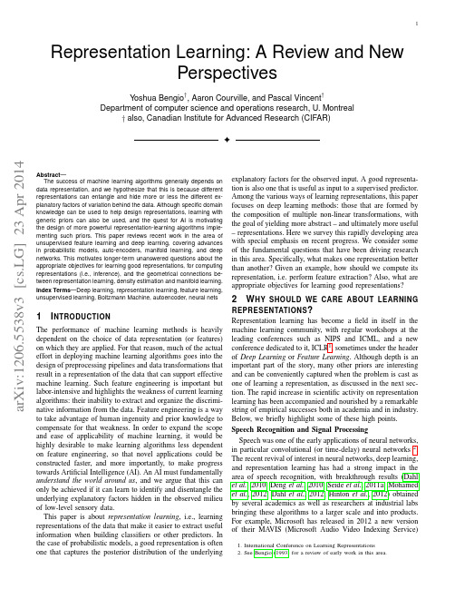
explanatory factors for the observed input. A good representation is also one that is useful as input to a supervised predictor. Among the various ways of learning representations, this paper focuses on deep learning methods: those that are formed by the composition of multiple non-linear transformations, with the goal of yielding more abstract – and ultimately more useful – representations. Here we survey this rapidly developing area with special emphasis on recent progress. We consider some of the fundamental questions that have been driving research in this area. Specifically, what makes one representation better than another? Given an example, how should we compute its representation, i.e. perform feature extraction? Also, what are appropriate objectives for learning good representations?
The advantages and disadvantages of semantic ambiguity

The Advantages and Disadvantages of Semantic Ambiguity Jennifer Rodd(jenni.rodd@)MRC Cognition and Brain Sciences Unit15Chaucer Road,Cambridge,UKGareth Gaskell(g.gaskell@)Department of PsychologyUniversity of York,York,UKWilliam Marslen-Wilson(william.marslen-wilson@)MRC Cognition and Brain Sciences Unit15Chaucer Road,Cambridge,UKAbstractThere have been several reports of faster lexical decisions for words that have many meanings(e.g.,ring)compared with words with few meanings(e.g.,hotel).However,it is not clear whether this advantage for ambiguous words arises because they have multiple unrelated meanings,or because they havea large number of highly related word senses.All current ac-counts of the ambiguity advantage assume that it is unrelated meanings that produce the processing benefit.We report two experiments that challenge this assumption;in visual and audi-tory lexical decision experiments we found that while multiple senses did produce faster responses,multiple meanings pro-duced a disadvantage.We discuss how models of word recog-nition could accommodate this new pattern of results.IntroductionMany words are semantically ambiguous,and can refer to more than one concept.For example,bark can refer either to a part of a tree,or to the sound made by a dog.To under-stand such words,we must disambiguate between these dif-ferent interpretations,normally on the basis of the context in which the word occurs.However,ambiguous words can also be recognised in isolation;when presented with a word like bark we are able to identify an appropriate meaning rapidly, and are often unaware of any other meanings.Words can be ambiguous in different ways.The two mean-ings of a word like bark are semantically unrelated,and seem to share the same written and spoken form purely by chance. Other words are ambiguous between highly related senses, which are systematically related to each other.For example, the word twist can refer to a bend in a road,an unexpected ending to a story,a type of dance,and other related concepts. The linguistic literature makes a distinction between these two types of ambiguity,and refers to them as homonymy and polysemy(Lyons,1977;Cruse,1986).Homonyms,such as the two meanings of bark,are said to be different words that by chance share the same orthographic and phonologi-cal form.On the other hand,a polysemous word like twist is considered to be a single word that has more than one sense. All standard dictionaries respect this distinction between word meanings and word senses;lexicographers routinely de-cide whether different usages of the same spelling should cor-respond to different lexical entries or different senses within a single entry.Many criteria(e.g.,etymological,semantic and syntactic)have been suggested to operationalise this distinc-tion between senses and meanings.However,it is generally agreed that while the distinction appears easy to formulate,it is difficult,to apply with consistency and reliability.People will often disagree about whether two usages of a word are sufficiently related that they should be taken as senses of a single meaning rather than different meanings.This suggests that these two types of ambiguity may be best viewed as the end points on a continuum.However,even if there is not a clear distinction between these two different types of ambigu-ity,it is important to remember that words that are described as ambiguous can vary between these two extremes.In this paper we will review the evidence on how lexical ambiguity affects the recognition of isolated words,and will argue that the distinction been these two qualitatively dif-ferent types of ambiguity has not been addressed.We then report two experiments that confirm the importance of the sense-meaning distinction,and show that in both the visual and the auditory domains the effects of word meanings and word senses are very different.The Ambiguity AdvantageIn early studies of semantic ambiguity,Rubenstein,Garfield, and Millikan(1970)and Jastrzembski(1981)reported faster visual lexical decisions for semantically ambiguous words than for unambiguous words.However,these studies did not control for the subjective familiarity of the words,and Gerns-bacher(1984)found no effect of ambiguity over and above familiarity.Since then,however,Kellas,Ferraro,and Simp-son(1988),Borowsky and Masson(1996)and Azuma and Van Orden(1997)have all reported an ambiguity advantage in visual lexical decision experiments using stimuli that were controlled for familiarity.Although there does seem to a consensus in the litera-ture that lexical ambiguity can produce faster lexical decision times,it is not at all clear what type of ambiguity is produc-ing the effect.Is it multiple meanings,or multiple senses that produces the advantage?One way of trying to answer this question is to examine the dictionary entries of the words used in these experiments.As described above,dictionaries make a distinction between words whose meanings are sufficiently unrelated that they are given multiple entries,and those thathave multiple senses within an entry.This provides a conve-nient way in which to categorise words as being ambiguous between multiple meanings or between multiple senses. Rodd,Gaskell,and Marslen-Wilson(1999)analyzed the stimuli used in the three studies that report a significant am-biguity advantage in this way,and found that for all three studies the high-ambiguity words have more word senses than the low-ambiguity words.Further,only in the Borowsky and Masson(1996)stimuli did the two groups differ in the num-ber of meanings.Therefore,it appears that it may be multiple senses rather than multiple meanings that are producing the ambiguity advantage.Despite this,all current explanations of the ambiguity advantage assume that the processing bene-fit arises because of the presence of unrelated meanings. Models of the Ambiguity AdvantageOne way that the ambiguity advantage has been explained has been to assume that ambiguous words have multiple en-tries within a lexical network.For example,(Kellas et al., 1988)suggest that the benefit arises because,while the mul-tiple entries for an ambiguous word do not inhibit each other, they both act independently to inhibit all other competing en-tries,and this increased inhibition of competitors produces the faster recognition times.Others have assumed that the benefit arises within this type of model by assuming that there is some level of noise or probabilistic activation(Jastrzembski,1981).Because words with multiple meanings are assumed to have multiple entries, these words might benefit from having more than one com-petitor in the race for recognition;on average,by a particular point in time,one of these competitors is more likely to have reached the threshold for recognition than a word that has only one entry in the race.Both these approaches to explaining the ambiguity advan-tage predict that the effect will occur whenever the different meanings of the ambiguous words are sufficiently unrelated to have separate entries in the mental lexicon;they make no specific predictions about what should happen for words with multiple senses,as it is not clear whether word senses would correspond to separate entries within the network.An alternative view of word recognition is that words com-pete to activate a representation of their meaning.There have been several recent models of both spoken and visual word recognition that have taken this approach(Hinton&Shal-lice,1991;Plaut&Shallice,1993;Joordens&Besner,1994; Gaskell&Marslen-Wilson,1997;Plaut,1997).These mod-els use distributed lexical representations;each word is repre-sented as a unique pattern of activation across a set of ortho-graphic/phonological and semantic units.Within models of this type,the orthographic pattern bark must be associated with two different semantic patterns corre-sponding to its two meanings.When the orthographic pattern is presented to the network,the network will try to instanti-ate the word’s two meanings across the same set of semantic units simultaneously.These competing semantic representa-tions will interfere with each other,and this interference is likely to increase the time it takes for a stable pattern of acti-vation to be produced.Therefore,it appears that these models predict that lexical ambiguity should delay recognition,and not produce the faster response times seen in the literature.In response to this inconsistency between the ambiguity ad-vantage literature and the predictions of semantic competition models,there have been several attempts to show that,given particular assumptions,this class of model can overcome the semantic competition effect,and show an advantage for am-biguous words(e.g.Joordens and Besner(1994),Borowsky and Masson(1996)and Kawamoto,Farrar,and Kello(1994)). Importantly,these models assume that the effect to be mod-elled is an advantage for those words with multiple unrelated meanings.Thus,the ambiguity advantage has been interpreted within a range of models of word recognition.However,all these accounts have implicitly assumed that the ambiguity advan-tage literature demonstrates that there is a processing advan-tage for words with more than one,unrelated,meaning.As discussed above,it is not clear that this is the case;the am-biguity advantage may be a benefit for words with multiple senses rather than multiple meanings.In order to understand fully the implications of semantic ambiguity for models of word recognition,we need to determine which of these ex-planations is correct.Experiment1:Visual Lexical Decision MethodExperimental Design This experiment attempts to separate out the effects of lexical ambiguity and multiple word senses by using a factorial design(see Table1).Groups of ambigu-ous and unambiguous words were selected to have either few or many senses on the basis of their dictionary entries.Table1:Experiment1:Experimental DesignAmbiguity Senses ExampleAmbiguous Few pupilAmbiguous Many slipUnambiguous Few cageUnambiguous Many maskParticipants The participants were25members of the MRC Cognition and Brain Sciences Unit subject panel. All had English as theirfirst language,and had normal or corrected-to-normal vision.Stimuli The word stimuli were selected to conform to a2x 2factorial design,where the two factors were ambiguity and number of senses.Words were classed as being unambiguous if they had only one entry in The Online Wordsmyth English Dictionary-Thesaurus(Parks,Ray,&Bland,1998),and as ambiguous if they had two or more entries.Two measures of the number of senses were used.These were the total number of word senses listed in the Wordsmyth dictionary for all the entries for that word,and the total number of senses given in the WordNet lexical database(Fellbaum,1998).Thirty-two stimuli were selected tofill each cell of the fac-torial design,such that the number of word meanings was matched across each level of number of word senses,and the total number of word senses was matched across each level of the number of word meanings.The four groups of words were matched for frequency in the CELEX lexical database(Baayen,Piepenbrock,&Van Rijn,1993),number of letters,number of syllables,con-creteness and familiarity.Concreteness and familiarity scores were obtained from rating pre-tests in which all the words were rated on a7-point scale by participants who were mem-bers of the MRC Cognition and Brain Sciences Unit subject panel,and who did not participate in the lexical decision ex-periment.The groups were not explicitly matched for neighbourhood density;however,the number of words in CELEX that dif-fered from each word by only one letter(;Coltheart,Dave-laar,Jonasson,&Besner,1977)was calculated for each word. An analysis of variance(ANOV A)showed that the words in the four groups did not differ significantly on this measure;,.The non-word distractors were pseudohomophones,such as brane,with a similar distribution of word lengths to the word stimuli.Pseudohomophones were used because both (Azuma&Van Orden,1997)and(Pexman&Lupker,1999) found stronger effects of semantic ambiguity when these non-words were used.In thisfirst experiment,we wanted to max-imise the chance offinding significant effects of ambiguity. Procedure All the stimulus items were pseudo-randomly divided into four lists,such that each list contained approxi-mately the same number of words from each stimulus group. Participants were presented with the four lists in a random or-der,with a short break between lists.Within the lists,the or-der in which stimulus items were presented was randomised for each participant.All participants saw all of the stimulus materials.A practice session,consisting of64items not used in the analysis,was given to familiarise participants with the task.Each block began with10stimuli not included in the analysis.For each of the word and non-word stimuli,the partici-pants were presented with afixation point in the centre of a computer screen for500msec,followed by the stimulus item. Their task was to decide whether each item was a word or a non-word;recognition was signalled with the dominant hand, non-recognition with the other hand.As soon as the partic-ipant responded,the word was replaced with a newfixation point.ResultsThe data from two participants were removed from the analy-sis,because of error rates greater than10%.The latencies for responses to the word and non-word stimuli were recorded, and the inverse of these response times(1/RT)were used in the analyses to minimize the effect of outliers(Ulrich& Miller,1994;Ratcliff,1993).Incorrect responses were not included in the analysis.The overall error rate for responses was3.6%.Mean values were calculated separately across participants and items.The participant means were subjected to an ANOV A,and the item means were subjected to an analysis of covariance(ANCOV A)with frequency,familiarity,concrete-ness and length entered as covariates.The mean response times are given in Figure1.The ANCOV A revealed significant effects of frequency,fa-miliarity,length and neighbourhood density(all). The effect of concreteness was non-significant(),so this variable was removed from the ANCOV A.The responsefew sensesmany senses Ambiguous words were responded to more slowly than un-ambiguous words.There was no significant interaction be-tween these two variables().The error data also showed a significant effect of the num-ber of senses;fewer errors were made for words with many senses(,;, ).In the error data neither the effect of ambiguity northe interaction between the two variables reached significance (all).DiscussionThis experiment shows that words with many senses were re-sponded to faster and with fewer errors that words with few senses.This advantage for multiple senses is in contrast with a disadvantage for words with multiple meanings.Although this disadvantage was not significant,it is clear that contrary to the accepted view in the literature,there is no process-ing advantage for words with multiple meanings.Moreover, Rodd et al.(1999)didfind a significant disadvantage in vi-sual lexical decision for words with more than one meaning, compared with unambiguous words,when the stimuli were selected to minimise the effect of word senses.Thus,previ-ous reports of an ambiguity advantage must be the result of the multiple senses of the high-ambiguity stimuli rather than their multiple meanings.Therefore,the results of this experiment together with the results of Rodd et al.(1999)show that the two types of lex-ical ambiguity have opposite effects on visual word recogni-tion;while ambiguity between multiple meanings may delay recognition,ambiguity between multiple senses is beneficial. The following experiment will investigate whether this pat-tern is also seen in the auditory domain.If the above pattern of data is telling us something interesting about the way in which word meanings are stored and processed,we should expect tofind the same pattern independent of the input modality.This experiment will also allow us to establish that theseeffects of semantic ambiguity are not contingent on the type of non-word distractors used.In Experiment1,pseudohomo-phones such as brane were used.There is still debate about how pseudohomophones affect lexical processing(see Pex-man&Lupker,1999for a review).One possibility is that they simply increase the difficulty of the task,and so increase sensitivity to relatively small effects.However,an alternative explanation is that pseudohomophones strategically effect the way that participants make use of orthographic,phonological and semantic information.The following experiment,which does not use pseudohomophones will attempt to demonstrate that these effects are not due to strategic effects induced by these particular non-words.Finally,this experiment will also allow us to try and repli-cate the significant ambiguity disadvantage seen by Rodd et al.(1999).Experiment2:Auditory Lexical Decision MethodExperimental Design The experimental design was identi-cal to Experiment1.Participants The participants were26students at Cam-bridge University who had not participated in thefirst experi-ment.All had English as theirfirst language,and had normal or corrected-to-normal vision.Stimuli23stimuli were selected tofill each cell of the fac-torial design,such that the number of word meanings was matched across each level of number of word senses.The words were selected on the basis of dictionary entries as in Experiment1.The number of words in each cell is smaller than was used in Experiment1,because of the additional con-straints used to match the groups.77%of the words were also used in Experiment1.The four groups of words were matched for frequency, number of phonemes,the phoneme at which the word be-comes unique,actual length of the words in msec,concrete-ness and familiarity.Concreteness and familiarity scores were obtained from the same rating pre-test as in Experiment 1.All the words had only one syllable.The non-word stimuli were created to be as word-like as possible,and to have a similar distribution of word lengths to the word stimuli.Procedure The procedure used was the same as that in Ex-periment1,except that now the stimuli were spoken words. Each item appeared1000ms after the participants’response to the preceding item.If the participant did not respond within3000ms of the onset of a word,the next item was presented.ResultsThe data from four participants were removed from the anal-ysis,because of error rates greater than10%.Incorrect re-sponses were not included in the analysis.The overall error rate for responses was5.8%.As in Experiment1,inverse response times were used in all analyses.Mean values were calculated separately across par-ticipants and items.The participant means were subjected to an analysis of variance(ANOV A),and the item means were subjected to an analysis of covariance(ANCOV A),with fa-miliarity and length entered as covariates.The mean responseunambiguousfew sensesmany senseslexical decisionsignificant effectscant in both the participants and items analysis(,;,).Words with many senses were responded to faster than words with few senses. The effect of ambiguity was also significant in both the par-ticipants analysis and the items analysis(, ;,).Ambiguous words were responded to more slowly than unambiguous words. The interaction between these two variables was marginal in the subjects analysis but did not approach significance in the items analysis(,;, ).The error data showed a similar pattern of results to the response time data.Fewer errors were made for words with many senses,although this difference was significant only in the subjects analysis but not in the items analysis; (,;,). Fewer errors were also made for unambiguous words,al-though this difference was only marginal in the subjects anal-ysis and did not approach significance in the items analysis; (,;,).The interaction between the two variables was not significant in either analysis().General DiscussionBoth the experiments reported here have shown an advantage for words with many word senses.This advantage for multi-ple senses was seen alongside a disadvantage for words with multiple meanings.This suggests that the ambiguity advan-tage reported in earlier studies must have been produced by the high number of related word senses of high-ambiguity stimuli,and not by their unrelated meanings.What are the implications of this new pattern of results for models of word recognition?Previously,these models hadbeen required to produce an advantage for words with multi-ple meanings,but our data suggests they must accommodate exactly the reverse effect.In fact,this is less problematic than might be expected.The ambiguity disadvantage can easily be explained by models in which words compete for the activation of seman-tic representations(Hinton&Shallice,1991;Plaut&Shal-lice,1993;Joordens&Besner,1994;Gaskell&Marslen-Wilson,1997;Plaut,1997).As discussed earlier,in these models competition between the different meanings of am-biguous words would delay their recognition.As noted by Jo-ordens and Besner(1994),an ambiguity advantage can only be produced by these models if an additional mechanism is present to overcome this semantic competition.These results suggest that no such mechanism is required.The other class of model that may be able to accommodate this new pattern of results is those models in which words compete to activate abstract word nodes within a lexical net-work.Earlier,we discussed how these models could produce an ambiguity advantage by assuming either that ambiguous words are more efficient at inhibiting competitors,or that they benefit from having multiple competitors in the race for recognition.Surprisingly,these models can just as easily accommodate a disadvantage for words with multiple meanings.As in all experiments of this type,the ambiguous words and unam-biguous words in these experiments were matched on total frequency.This means that the frequency of each meaning of the ambiguous words is on average half that of the unambigu-ous word.This frequency difference could produce faster lex-ical decisions for the unambiguous words.Similarly,if lateral inhibition were present between all word nodes,including the nodes corresponding to the different meanings of an ambigu-ous word,this would act to slow the recognition of ambiguous words.Therefore,it appears that both classes of models consid-ered here can be modified to accommodate thefinding of slower responses to words with more than one unrelated meaning.However,Rodd et al.(1999)have shown that at least in the visual domain,the ambiguity disadvantage is modulated by the rated relatedness of the two meanings of the ambiguous words;words whose meanings are sufficiently different to be considered meanings rather than senses but whose meanings are mildly related are responded to more quickly that those whose meanings are highly unrelated.This suggests that semantic representations are actively involved in the process that produces the ambiguity disadvantage,and that the effect cannot be explained solely as the result of a frequency bias for unambiguous words or lateral inhibition between abstract word nodes.Therefore,the ambiguity dis-advantage may more easily be explained as the result of se-mantic competition which is maximal when the competing representations are unrelated.It is therefore apparently straightforward to explain the ob-served ambiguity disadvantage.The intriguing question that remains is what causes the advantage for words with many senses?One possibility is to explain this effect in terms of the attractor basins that develop in a distributed semantic net-work.The different senses of a word correspond to a set of highly correlated patterns of semantic activation.As noted by Kawamoto(1993),for a word with many related senses, these senses will create a broad and shallow basin of attrac-tion,containing more than one stable state corresponding to each different sense.It is plausible that within certain archi-tectures,settling into the correct attractor may be quicker for such a broad attractor,compared with the attractor of a word with few senses,or that the multiple stable states within the attractor may lead to faster settling times.This suggestion needs to be assessed by performing the appropriate simula-tions.A second possible explanation of the sense effect would be to consider the difference between words with many and few senses as reflecting a difference in the amount of semantic in-formation associated with the two types of words.In other words,a word with many senses may be considered to be se-mantically rich.This is essentially the same argument that Plaut and Shallice(1993)put forward to account for the pro-cessing benefit of concrete words over abstract words.In their computational account of the concreteness effect,the differ-ence between abstract and concrete words is reflected in the number of semantic features in a distributed semantic repre-sentation;abstract words are given fewer semantic features than concrete words.This results in concrete words activat-ing more stable representations than abstract words.These stable representations lead in turn to faster settling times for words with more semantic features.It is not yet possible to distinguish between these(and other)possible explanations of the sense effect reported here.A combination of network simulations and further experi-ments is required to determine how existing models of word recognition should be modified to accommodate the benefit for words with many word senses.What is clear is that the distinction we have emphasised between word meanings and word senses is critical.In the past,ambiguity has been treated as a unitary property of words;we have shown that this has masked an informative pattern of results that can be used to constrain models of how words are recognised.More generally,these experiments emphasise how word recognition is inextricably linked with word meanings.Data of this kind places an increasing demand on models of word recognition to incorporate richer semantic representations that reflect the complex structures of the meanings of words.ReferencesAzuma,T.,&Van Orden,G.C.(1997).Why safe is better than fast:The relatedness of a word’s meanings affects lex-ical decision times.Journal of Memory and Language,36, 484–504.Baayen,R.H.,Piepenbrock,R.,&Van Rijn,H.(1993).The CELEX Lexical Database.CD-ROM.Philadelphia,P.A: Linguistic Data Consortium,University of Pennsylvania. Borowsky,R.,&Masson,M.E.J.(1996).Semantic ambigu-ity effects in word identification.Journal of Experimental Psychology:Learning Memory and Cognition,22,63–85. Coltheart,M.,Davelaar,E.,Jonasson,J.T.,&Besner,D. (1977).Access to the internal lexicon.In S.Dornic(Ed.), Attention and Performance VI(pp.535–555).Hillsdale, NJ:Erlbaum.Cruse,A.D.(1986).Lexical semantics.Cambridge,England: Cambridge University Press.Fellbaum,C.(Ed.).(1998).Wordnet:An electronic lexical database.Cambridge,MA:MIT Press.Gaskell,M.G.,&Marslen-Wilson,W.D.(1997).Integrating form and meaning:A distributed model of speech nguage and Cognitive Processes,12,613–656. Gernsbacher,M.A.(1984).Resolving20years of inconsis-tent interactions between lexical familiarity and orthogra-phy,concreteness,and polysemy.Journal of Experimental Psychology:General,113,254–281.Hinton,G.E.,&Shallice,T.(1991).Lesioning an attractor network:Investigations of acquired dyslexia.Psychologi-cal Review,98,74–95.Jastrzembski,J.E.(1981).Multiple meanings,number of related meanings,frequency of occurrence,and the lexicon. Cognitive Psychology,13,278–305.Joordens,S.,&Besner,D.(1994).When banking on mean-ing is not(yet)money in the bank-explorations in con-nectionist modeling.Journal of Experimental Psychology: Learning Memory and Cognition,20,1051–1062. Kawamoto,A.H.(1993).Nonlinear dynamics in the resolu-tion of lexical ambiguity:a parallel distributed processing account.Journal of Memory and Language,32,474–516. Kawamoto,A.H.,Farrar,W.T.,&Kello,C.T.(1994).When two meanings are better than one:Modeling the ambiguity advantage using a recurrent distributed network.Journal of Experimental Psychology:Human Perception and Perfor-mance,20,1233–1247.Kellas,G.,Ferraro,F.R.,&Simpson,G.B.(1988).Lexi-cal ambiguity and the timecourse of attentional allocation in word recognition.Journal of Experimental Psychology: Human Perception and Performance,14,601–609. Lyons,J.(1977).Semantics.Cambridge,England:Cam-bridge University Press.Parks,R.,Ray,J.,&Bland,S.(1998).Wordsmyth English dictionary-thesaurus.[ONLINE].Available:http: ///[1999,February1],University of Chicago.Pexman,P.M.,&Lupker,S.J.(1999).Ambiguity and visual word recognition:Can feedback explain both homophone and polysemy effects?Canadian Journal of Experimental Psychology,323–334.Plaut,D.C.(1997).Structure and function in the lexical system:insights from distributed models of word reading and lexical nguage and Cognitive Processes, 12,765–805.Plaut,D.C.,&Shallice,T.(1993).Deep dyslexia:A case study of connectionist neuropsychology.Cognitive Neu-ropsychology,10,377–500.Ratcliff,R.(1993).Methods for dealing with reaction-time outliers.Psychological Bulletin,114(3),510-532. Rodd,J.M.,Gaskell,M.G.,&Marslen-Wilson,W.D. (1999).Semantic competition and the ambiguity dis-advantage.In M.Hahn&S. C.Stoness(Eds.), Proceedings of the Twenty First Annual Conference of the Cognitive Science Society(pp.608–613).Mahwah,New Jersey:Lawrence Erlbaum Associates.Rubenstein,H.,Garfield,L.,&Millikan,J.A.(1970).Ho-mographic entries in the internal lexicon.Journal of Verbal Learning and Verbal Behavior,9,487–494.Ulrich,R.,&Miller,J.(1994).Effects of trunca-tion on reaction-time analysis.Journal of Experimental Psychology-General,123(1),34-80.。
Learning Recurrent Neural Networks with Hessian-Free Optimization

1. Introduction
A Recurrent Neural Network (RNN) is a neural network that operates in time. At each timestep, it accepts an input vector, updates its (possibly high-dimensional) hidden state via non-linear activation functions, and uses it to make a prediction of its output. RNNs form a rich model class because their hidden state can store information as high-dimensional distributed representations (as opposed to a Hidden Markov Model, whose hidden state is essentially log n-dimensional) and their nonlinear dynamics can implement rich and powerful computations, allowing the RNN to perform modeling and prediction tasks for sequences with highly complex structure.
《神经网络与深度学习综述DeepLearning15May2014
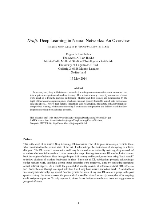
Draft:Deep Learning in Neural Networks:An OverviewTechnical Report IDSIA-03-14/arXiv:1404.7828(v1.5)[cs.NE]J¨u rgen SchmidhuberThe Swiss AI Lab IDSIAIstituto Dalle Molle di Studi sull’Intelligenza ArtificialeUniversity of Lugano&SUPSIGalleria2,6928Manno-LuganoSwitzerland15May2014AbstractIn recent years,deep artificial neural networks(including recurrent ones)have won numerous con-tests in pattern recognition and machine learning.This historical survey compactly summarises relevantwork,much of it from the previous millennium.Shallow and deep learners are distinguished by thedepth of their credit assignment paths,which are chains of possibly learnable,causal links between ac-tions and effects.I review deep supervised learning(also recapitulating the history of backpropagation),unsupervised learning,reinforcement learning&evolutionary computation,and indirect search for shortprograms encoding deep and large networks.PDF of earlier draft(v1):http://www.idsia.ch/∼juergen/DeepLearning30April2014.pdfLATEX source:http://www.idsia.ch/∼juergen/DeepLearning30April2014.texComplete BIBTEXfile:http://www.idsia.ch/∼juergen/bib.bibPrefaceThis is the draft of an invited Deep Learning(DL)overview.One of its goals is to assign credit to those who contributed to the present state of the art.I acknowledge the limitations of attempting to achieve this goal.The DL research community itself may be viewed as a continually evolving,deep network of scientists who have influenced each other in complex ways.Starting from recent DL results,I tried to trace back the origins of relevant ideas through the past half century and beyond,sometimes using“local search”to follow citations of citations backwards in time.Since not all DL publications properly acknowledge earlier relevant work,additional global search strategies were employed,aided by consulting numerous neural network experts.As a result,the present draft mostly consists of references(about800entries so far).Nevertheless,through an expert selection bias I may have missed important work.A related bias was surely introduced by my special familiarity with the work of my own DL research group in the past quarter-century.For these reasons,the present draft should be viewed as merely a snapshot of an ongoing credit assignment process.To help improve it,please do not hesitate to send corrections and suggestions to juergen@idsia.ch.Contents1Introduction to Deep Learning(DL)in Neural Networks(NNs)3 2Event-Oriented Notation for Activation Spreading in FNNs/RNNs3 3Depth of Credit Assignment Paths(CAPs)and of Problems4 4Recurring Themes of Deep Learning54.1Dynamic Programming(DP)for DL (5)4.2Unsupervised Learning(UL)Facilitating Supervised Learning(SL)and RL (6)4.3Occam’s Razor:Compression and Minimum Description Length(MDL) (6)4.4Learning Hierarchical Representations Through Deep SL,UL,RL (6)4.5Fast Graphics Processing Units(GPUs)for DL in NNs (6)5Supervised NNs,Some Helped by Unsupervised NNs75.11940s and Earlier (7)5.2Around1960:More Neurobiological Inspiration for DL (7)5.31965:Deep Networks Based on the Group Method of Data Handling(GMDH) (8)5.41979:Convolution+Weight Replication+Winner-Take-All(WTA) (8)5.51960-1981and Beyond:Development of Backpropagation(BP)for NNs (8)5.5.1BP for Weight-Sharing Feedforward NNs(FNNs)and Recurrent NNs(RNNs)..95.6Late1980s-2000:Numerous Improvements of NNs (9)5.6.1Ideas for Dealing with Long Time Lags and Deep CAPs (10)5.6.2Better BP Through Advanced Gradient Descent (10)5.6.3Discovering Low-Complexity,Problem-Solving NNs (11)5.6.4Potential Benefits of UL for SL (11)5.71987:UL Through Autoencoder(AE)Hierarchies (12)5.81989:BP for Convolutional NNs(CNNs) (13)5.91991:Fundamental Deep Learning Problem of Gradient Descent (13)5.101991:UL-Based History Compression Through a Deep Hierarchy of RNNs (14)5.111992:Max-Pooling(MP):Towards MPCNNs (14)5.121994:Contest-Winning Not So Deep NNs (15)5.131995:Supervised Recurrent Very Deep Learner(LSTM RNN) (15)5.142003:More Contest-Winning/Record-Setting,Often Not So Deep NNs (16)5.152006/7:Deep Belief Networks(DBNs)&AE Stacks Fine-Tuned by BP (17)5.162006/7:Improved CNNs/GPU-CNNs/BP-Trained MPCNNs (17)5.172009:First Official Competitions Won by RNNs,and with MPCNNs (18)5.182010:Plain Backprop(+Distortions)on GPU Yields Excellent Results (18)5.192011:MPCNNs on GPU Achieve Superhuman Vision Performance (18)5.202011:Hessian-Free Optimization for RNNs (19)5.212012:First Contests Won on ImageNet&Object Detection&Segmentation (19)5.222013-:More Contests and Benchmark Records (20)5.22.1Currently Successful Supervised Techniques:LSTM RNNs/GPU-MPCNNs (21)5.23Recent Tricks for Improving SL Deep NNs(Compare Sec.5.6.2,5.6.3) (21)5.24Consequences for Neuroscience (22)5.25DL with Spiking Neurons? (22)6DL in FNNs and RNNs for Reinforcement Learning(RL)236.1RL Through NN World Models Yields RNNs With Deep CAPs (23)6.2Deep FNNs for Traditional RL and Markov Decision Processes(MDPs) (24)6.3Deep RL RNNs for Partially Observable MDPs(POMDPs) (24)6.4RL Facilitated by Deep UL in FNNs and RNNs (25)6.5Deep Hierarchical RL(HRL)and Subgoal Learning with FNNs and RNNs (25)6.6Deep RL by Direct NN Search/Policy Gradients/Evolution (25)6.7Deep RL by Indirect Policy Search/Compressed NN Search (26)6.8Universal RL (27)7Conclusion271Introduction to Deep Learning(DL)in Neural Networks(NNs) Which modifiable components of a learning system are responsible for its success or failure?What changes to them improve performance?This has been called the fundamental credit assignment problem(Minsky, 1963).There are general credit assignment methods for universal problem solvers that are time-optimal in various theoretical senses(Sec.6.8).The present survey,however,will focus on the narrower,but now commercially important,subfield of Deep Learning(DL)in Artificial Neural Networks(NNs).We are interested in accurate credit assignment across possibly many,often nonlinear,computational stages of NNs.Shallow NN-like models have been around for many decades if not centuries(Sec.5.1).Models with several successive nonlinear layers of neurons date back at least to the1960s(Sec.5.3)and1970s(Sec.5.5). An efficient gradient descent method for teacher-based Supervised Learning(SL)in discrete,differentiable networks of arbitrary depth called backpropagation(BP)was developed in the1960s and1970s,and ap-plied to NNs in1981(Sec.5.5).BP-based training of deep NNs with many layers,however,had been found to be difficult in practice by the late1980s(Sec.5.6),and had become an explicit research subject by the early1990s(Sec.5.9).DL became practically feasible to some extent through the help of Unsupervised Learning(UL)(e.g.,Sec.5.10,5.15).The1990s and2000s also saw many improvements of purely super-vised DL(Sec.5).In the new millennium,deep NNs havefinally attracted wide-spread attention,mainly by outperforming alternative machine learning methods such as kernel machines(Vapnik,1995;Sch¨o lkopf et al.,1998)in numerous important applications.In fact,supervised deep NNs have won numerous of-ficial international pattern recognition competitions(e.g.,Sec.5.17,5.19,5.21,5.22),achieving thefirst superhuman visual pattern recognition results in limited domains(Sec.5.19).Deep NNs also have become relevant for the more generalfield of Reinforcement Learning(RL)where there is no supervising teacher (Sec.6).Both feedforward(acyclic)NNs(FNNs)and recurrent(cyclic)NNs(RNNs)have won contests(Sec.5.12,5.14,5.17,5.19,5.21,5.22).In a sense,RNNs are the deepest of all NNs(Sec.3)—they are general computers more powerful than FNNs,and can in principle create and process memories of ar-bitrary sequences of input patterns(e.g.,Siegelmann and Sontag,1991;Schmidhuber,1990a).Unlike traditional methods for automatic sequential program synthesis(e.g.,Waldinger and Lee,1969;Balzer, 1985;Soloway,1986;Deville and Lau,1994),RNNs can learn programs that mix sequential and parallel information processing in a natural and efficient way,exploiting the massive parallelism viewed as crucial for sustaining the rapid decline of computation cost observed over the past75years.The rest of this paper is structured as follows.Sec.2introduces a compact,event-oriented notation that is simple yet general enough to accommodate both FNNs and RNNs.Sec.3introduces the concept of Credit Assignment Paths(CAPs)to measure whether learning in a given NN application is of the deep or shallow type.Sec.4lists recurring themes of DL in SL,UL,and RL.Sec.5focuses on SL and UL,and on how UL can facilitate SL,although pure SL has become dominant in recent competitions(Sec.5.17-5.22). Sec.5is arranged in a historical timeline format with subsections on important inspirations and technical contributions.Sec.6on deep RL discusses traditional Dynamic Programming(DP)-based RL combined with gradient-based search techniques for SL or UL in deep NNs,as well as general methods for direct and indirect search in the weight space of deep FNNs and RNNs,including successful policy gradient and evolutionary methods.2Event-Oriented Notation for Activation Spreading in FNNs/RNNs Throughout this paper,let i,j,k,t,p,q,r denote positive integer variables assuming ranges implicit in the given contexts.Let n,m,T denote positive integer constants.An NN’s topology may change over time(e.g.,Fahlman,1991;Ring,1991;Weng et al.,1992;Fritzke, 1994).At any given moment,it can be described as afinite subset of units(or nodes or neurons)N= {u1,u2,...,}and afinite set H⊆N×N of directed edges or connections between nodes.FNNs are acyclic graphs,RNNs cyclic.Thefirst(input)layer is the set of input units,a subset of N.In FNNs,the k-th layer(k>1)is the set of all nodes u∈N such that there is an edge path of length k−1(but no longer path)between some input unit and u.There may be shortcut connections between distant layers.The NN’s behavior or program is determined by a set of real-valued,possibly modifiable,parameters or weights w i(i=1,...,n).We now focus on a singlefinite episode or epoch of information processing and activation spreading,without learning through weight changes.The following slightly unconventional notation is designed to compactly describe what is happening during the runtime of the system.During an episode,there is a partially causal sequence x t(t=1,...,T)of real values that I call events.Each x t is either an input set by the environment,or the activation of a unit that may directly depend on other x k(k<t)through a current NN topology-dependent set in t of indices k representing incoming causal connections or links.Let the function v encode topology information and map such event index pairs(k,t)to weight indices.For example,in the non-input case we may have x t=f t(net t)with real-valued net t= k∈in t x k w v(k,t)(additive case)or net t= k∈in t x k w v(k,t)(multiplicative case), where f t is a typically nonlinear real-valued activation function such as tanh.In many recent competition-winning NNs(Sec.5.19,5.21,5.22)there also are events of the type x t=max k∈int (x k);some networktypes may also use complex polynomial activation functions(Sec.5.3).x t may directly affect certain x k(k>t)through outgoing connections or links represented through a current set out t of indices k with t∈in k.Some non-input events are called output events.Note that many of the x t may refer to different,time-varying activations of the same unit in sequence-processing RNNs(e.g.,Williams,1989,“unfolding in time”),or also in FNNs sequentially exposed to time-varying input patterns of a large training set encoded as input events.During an episode,the same weight may get reused over and over again in topology-dependent ways,e.g.,in RNNs,or in convolutional NNs(Sec.5.4,5.8).I call this weight sharing across space and/or time.Weight sharing may greatly reduce the NN’s descriptive complexity,which is the number of bits of information required to describe the NN (Sec.4.3).In Supervised Learning(SL),certain NN output events x t may be associated with teacher-given,real-valued labels or targets d t yielding errors e t,e.g.,e t=1/2(x t−d t)2.A typical goal of supervised NN training is tofind weights that yield episodes with small total error E,the sum of all such e t.The hope is that the NN will generalize well in later episodes,causing only small errors on previously unseen sequences of input events.Many alternative error functions for SL and UL are possible.SL assumes that input events are independent of earlier output events(which may affect the environ-ment through actions causing subsequent perceptions).This assumption does not hold in the broaderfields of Sequential Decision Making and Reinforcement Learning(RL)(Kaelbling et al.,1996;Sutton and Barto, 1998;Hutter,2005)(Sec.6).In RL,some of the input events may encode real-valued reward signals given by the environment,and a typical goal is tofind weights that yield episodes with a high sum of reward signals,through sequences of appropriate output actions.Sec.5.5will use the notation above to compactly describe a central algorithm of DL,namely,back-propagation(BP)for supervised weight-sharing FNNs and RNNs.(FNNs may be viewed as RNNs with certainfixed zero weights.)Sec.6will address the more general RL case.3Depth of Credit Assignment Paths(CAPs)and of ProblemsTo measure whether credit assignment in a given NN application is of the deep or shallow type,I introduce the concept of Credit Assignment Paths or CAPs,which are chains of possibly causal links between events.Let usfirst focus on SL.Consider two events x p and x q(1≤p<q≤T).Depending on the appli-cation,they may have a Potential Direct Causal Connection(PDCC)expressed by the Boolean predicate pdcc(p,q),which is true if and only if p∈in q.Then the2-element list(p,q)is defined to be a CAP from p to q(a minimal one).A learning algorithm may be allowed to change w v(p,q)to improve performance in future episodes.More general,possibly indirect,Potential Causal Connections(PCC)are expressed by the recursively defined Boolean predicate pcc(p,q),which in the SL case is true only if pdcc(p,q),or if pcc(p,k)for some k and pdcc(k,q).In the latter case,appending q to any CAP from p to k yields a CAP from p to q(this is a recursive definition,too).The set of such CAPs may be large but isfinite.Note that the same weight may affect many different PDCCs between successive events listed by a given CAP,e.g.,in the case of RNNs, or weight-sharing FNNs.Suppose a CAP has the form(...,k,t,...,q),where k and t(possibly t=q)are thefirst successive elements with modifiable w v(k,t).Then the length of the suffix list(t,...,q)is called the CAP’s depth (which is0if there are no modifiable links at all).This depth limits how far backwards credit assignment can move down the causal chain tofind a modifiable weight.1Suppose an episode and its event sequence x1,...,x T satisfy a computable criterion used to decide whether a given problem has been solved(e.g.,total error E below some threshold).Then the set of used weights is called a solution to the problem,and the depth of the deepest CAP within the sequence is called the solution’s depth.There may be other solutions(yielding different event sequences)with different depths.Given somefixed NN topology,the smallest depth of any solution is called the problem’s depth.Sometimes we also speak of the depth of an architecture:SL FNNs withfixed topology imply a problem-independent maximal problem depth bounded by the number of non-input layers.Certain SL RNNs withfixed weights for all connections except those to output units(Jaeger,2001;Maass et al.,2002; Jaeger,2004;Schrauwen et al.,2007)have a maximal problem depth of1,because only thefinal links in the corresponding CAPs are modifiable.In general,however,RNNs may learn to solve problems of potentially unlimited depth.Note that the definitions above are solely based on the depths of causal chains,and agnostic of the temporal distance between events.For example,shallow FNNs perceiving large“time windows”of in-put events may correctly classify long input sequences through appropriate output events,and thus solve shallow problems involving long time lags between relevant events.At which problem depth does Shallow Learning end,and Deep Learning begin?Discussions with DL experts have not yet yielded a conclusive response to this question.Instead of committing myself to a precise answer,let me just define for the purposes of this overview:problems of depth>10require Very Deep Learning.The difficulty of a problem may have little to do with its depth.Some NNs can quickly learn to solve certain deep problems,e.g.,through random weight guessing(Sec.5.9)or other types of direct search (Sec.6.6)or indirect search(Sec.6.7)in weight space,or through training an NNfirst on shallow problems whose solutions may then generalize to deep problems,or through collapsing sequences of(non)linear operations into a single(non)linear operation—but see an analysis of non-trivial aspects of deep linear networks(Baldi and Hornik,1994,Section B).In general,however,finding an NN that precisely models a given training set is an NP-complete problem(Judd,1990;Blum and Rivest,1992),also in the case of deep NNs(S´ıma,1994;de Souto et al.,1999;Windisch,2005);compare a survey of negative results(S´ıma, 2002,Section1).Above we have focused on SL.In the more general case of RL in unknown environments,pcc(p,q) is also true if x p is an output event and x q any later input event—any action may affect the environment and thus any later perception.(In the real world,the environment may even influence non-input events computed on a physical hardware entangled with the entire universe,but this is ignored here.)It is possible to model and replace such unmodifiable environmental PCCs through a part of the NN that has already learned to predict(through some of its units)input events(including reward signals)from former input events and actions(Sec.6.1).Its weights are frozen,but can help to assign credit to other,still modifiable weights used to compute actions(Sec.6.1).This approach may lead to very deep CAPs though.Some DL research is about automatically rephrasing problems such that their depth is reduced(Sec.4). In particular,sometimes UL is used to make SL problems less deep,e.g.,Sec.5.10.Often Dynamic Programming(Sec.4.1)is used to facilitate certain traditional RL problems,e.g.,Sec.6.2.Sec.5focuses on CAPs for SL,Sec.6on the more complex case of RL.4Recurring Themes of Deep Learning4.1Dynamic Programming(DP)for DLOne recurring theme of DL is Dynamic Programming(DP)(Bellman,1957),which can help to facili-tate credit assignment under certain assumptions.For example,in SL NNs,backpropagation itself can 1An alternative would be to count only modifiable links when measuring depth.In many typical NN applications this would not make a difference,but in some it would,e.g.,Sec.6.1.be viewed as a DP-derived method(Sec.5.5).In traditional RL based on strong Markovian assumptions, DP-derived methods can help to greatly reduce problem depth(Sec.6.2).DP algorithms are also essen-tial for systems that combine concepts of NNs and graphical models,such as Hidden Markov Models (HMMs)(Stratonovich,1960;Baum and Petrie,1966)and Expectation Maximization(EM)(Dempster et al.,1977),e.g.,(Bottou,1991;Bengio,1991;Bourlard and Morgan,1994;Baldi and Chauvin,1996; Jordan and Sejnowski,2001;Bishop,2006;Poon and Domingos,2011;Dahl et al.,2012;Hinton et al., 2012a).4.2Unsupervised Learning(UL)Facilitating Supervised Learning(SL)and RL Another recurring theme is how UL can facilitate both SL(Sec.5)and RL(Sec.6).UL(Sec.5.6.4) is normally used to encode raw incoming data such as video or speech streams in a form that is more convenient for subsequent goal-directed learning.In particular,codes that describe the original data in a less redundant or more compact way can be fed into SL(Sec.5.10,5.15)or RL machines(Sec.6.4),whose search spaces may thus become smaller(and whose CAPs shallower)than those necessary for dealing with the raw data.UL is closely connected to the topics of regularization and compression(Sec.4.3,5.6.3). 4.3Occam’s Razor:Compression and Minimum Description Length(MDL) Occam’s razor favors simple solutions over complex ones.Given some programming language,the prin-ciple of Minimum Description Length(MDL)can be used to measure the complexity of a solution candi-date by the length of the shortest program that computes it(e.g.,Solomonoff,1964;Kolmogorov,1965b; Chaitin,1966;Wallace and Boulton,1968;Levin,1973a;Rissanen,1986;Blumer et al.,1987;Li and Vit´a nyi,1997;Gr¨u nwald et al.,2005).Some methods explicitly take into account program runtime(Al-lender,1992;Watanabe,1992;Schmidhuber,2002,1995);many consider only programs with constant runtime,written in non-universal programming languages(e.g.,Rissanen,1986;Hinton and van Camp, 1993).In the NN case,the MDL principle suggests that low NN weight complexity corresponds to high NN probability in the Bayesian view(e.g.,MacKay,1992;Buntine and Weigend,1991;De Freitas,2003), and to high generalization performance(e.g.,Baum and Haussler,1989),without overfitting the training data.Many methods have been proposed for regularizing NNs,that is,searching for solution-computing, low-complexity SL NNs(Sec.5.6.3)and RL NNs(Sec.6.7).This is closely related to certain UL methods (Sec.4.2,5.6.4).4.4Learning Hierarchical Representations Through Deep SL,UL,RLMany methods of Good Old-Fashioned Artificial Intelligence(GOFAI)(Nilsson,1980)as well as more recent approaches to AI(Russell et al.,1995)and Machine Learning(Mitchell,1997)learn hierarchies of more and more abstract data representations.For example,certain methods of syntactic pattern recog-nition(Fu,1977)such as grammar induction discover hierarchies of formal rules to model observations. The partially(un)supervised Automated Mathematician/EURISKO(Lenat,1983;Lenat and Brown,1984) continually learns concepts by combining previously learnt concepts.Such hierarchical representation learning(Ring,1994;Bengio et al.,2013;Deng and Yu,2014)is also a recurring theme of DL NNs for SL (Sec.5),UL-aided SL(Sec.5.7,5.10,5.15),and hierarchical RL(Sec.6.5).Often,abstract hierarchical representations are natural by-products of data compression(Sec.4.3),e.g.,Sec.5.10.4.5Fast Graphics Processing Units(GPUs)for DL in NNsWhile the previous millennium saw several attempts at creating fast NN-specific hardware(e.g.,Jackel et al.,1990;Faggin,1992;Ramacher et al.,1993;Widrow et al.,1994;Heemskerk,1995;Korkin et al., 1997;Urlbe,1999),and at exploiting standard hardware(e.g.,Anguita et al.,1994;Muller et al.,1995; Anguita and Gomes,1996),the new millennium brought a DL breakthrough in form of cheap,multi-processor graphics cards or GPUs.GPUs are widely used for video games,a huge and competitive market that has driven down hardware prices.GPUs excel at fast matrix and vector multiplications required not only for convincing virtual realities but also for NN training,where they can speed up learning by a factorof50and more.Some of the GPU-based FNN implementations(Sec.5.16-5.19)have greatly contributed to recent successes in contests for pattern recognition(Sec.5.19-5.22),image segmentation(Sec.5.21), and object detection(Sec.5.21-5.22).5Supervised NNs,Some Helped by Unsupervised NNsThe main focus of current practical applications is on Supervised Learning(SL),which has dominated re-cent pattern recognition contests(Sec.5.17-5.22).Several methods,however,use additional Unsupervised Learning(UL)to facilitate SL(Sec.5.7,5.10,5.15).It does make sense to treat SL and UL in the same section:often gradient-based methods,such as BP(Sec.5.5.1),are used to optimize objective functions of both UL and SL,and the boundary between SL and UL may blur,for example,when it comes to time series prediction and sequence classification,e.g.,Sec.5.10,5.12.A historical timeline format will help to arrange subsections on important inspirations and techni-cal contributions(although such a subsection may span a time interval of many years).Sec.5.1briefly mentions early,shallow NN models since the1940s,Sec.5.2additional early neurobiological inspiration relevant for modern Deep Learning(DL).Sec.5.3is about GMDH networks(since1965),perhaps thefirst (feedforward)DL systems.Sec.5.4is about the relatively deep Neocognitron NN(1979)which is similar to certain modern deep FNN architectures,as it combines convolutional NNs(CNNs),weight pattern repli-cation,and winner-take-all(WTA)mechanisms.Sec.5.5uses the notation of Sec.2to compactly describe a central algorithm of DL,namely,backpropagation(BP)for supervised weight-sharing FNNs and RNNs. It also summarizes the history of BP1960-1981and beyond.Sec.5.6describes problems encountered in the late1980s with BP for deep NNs,and mentions several ideas from the previous millennium to overcome them.Sec.5.7discusses afirst hierarchical stack of coupled UL-based Autoencoders(AEs)—this concept resurfaced in the new millennium(Sec.5.15).Sec.5.8is about applying BP to CNNs,which is important for today’s DL applications.Sec.5.9explains BP’s Fundamental DL Problem(of vanishing/exploding gradients)discovered in1991.Sec.5.10explains how a deep RNN stack of1991(the History Compressor) pre-trained by UL helped to solve previously unlearnable DL benchmarks requiring Credit Assignment Paths(CAPs,Sec.3)of depth1000and more.Sec.5.11discusses a particular WTA method called Max-Pooling(MP)important in today’s DL FNNs.Sec.5.12mentions afirst important contest won by SL NNs in1994.Sec.5.13describes a purely supervised DL RNN(Long Short-Term Memory,LSTM)for problems of depth1000and more.Sec.5.14mentions an early contest of2003won by an ensemble of shallow NNs, as well as good pattern recognition results with CNNs and LSTM RNNs(2003).Sec.5.15is mostly about Deep Belief Networks(DBNs,2006)and related stacks of Autoencoders(AEs,Sec.5.7)pre-trained by UL to facilitate BP-based SL.Sec.5.16mentions thefirst BP-trained MPCNNs(2007)and GPU-CNNs(2006). Sec.5.17-5.22focus on official competitions with secret test sets won by(mostly purely supervised)DL NNs since2009,in sequence recognition,image classification,image segmentation,and object detection. Many RNN results depended on LSTM(Sec.5.13);many FNN results depended on GPU-based FNN code developed since2004(Sec.5.16,5.17,5.18,5.19),in particular,GPU-MPCNNs(Sec.5.19).5.11940s and EarlierNN research started in the1940s(e.g.,McCulloch and Pitts,1943;Hebb,1949);compare also later work on learning NNs(Rosenblatt,1958,1962;Widrow and Hoff,1962;Grossberg,1969;Kohonen,1972; von der Malsburg,1973;Narendra and Thathatchar,1974;Willshaw and von der Malsburg,1976;Palm, 1980;Hopfield,1982).In a sense NNs have been around even longer,since early supervised NNs were essentially variants of linear regression methods going back at least to the early1800s(e.g.,Legendre, 1805;Gauss,1809,1821).Early NNs had a maximal CAP depth of1(Sec.3).5.2Around1960:More Neurobiological Inspiration for DLSimple cells and complex cells were found in the cat’s visual cortex(e.g.,Hubel and Wiesel,1962;Wiesel and Hubel,1959).These cellsfire in response to certain properties of visual sensory inputs,such as theorientation of plex cells exhibit more spatial invariance than simple cells.This inspired later deep NN architectures(Sec.5.4)used in certain modern award-winning Deep Learners(Sec.5.19-5.22).5.31965:Deep Networks Based on the Group Method of Data Handling(GMDH) Networks trained by the Group Method of Data Handling(GMDH)(Ivakhnenko and Lapa,1965; Ivakhnenko et al.,1967;Ivakhnenko,1968,1971)were perhaps thefirst DL systems of the Feedforward Multilayer Perceptron type.The units of GMDH nets may have polynomial activation functions imple-menting Kolmogorov-Gabor polynomials(more general than traditional NN activation functions).Given a training set,layers are incrementally grown and trained by regression analysis,then pruned with the help of a separate validation set(using today’s terminology),where Decision Regularisation is used to weed out superfluous units.The numbers of layers and units per layer can be learned in problem-dependent fashion. This is a good example of hierarchical representation learning(Sec.4.4).There have been numerous ap-plications of GMDH-style networks,e.g.(Ikeda et al.,1976;Farlow,1984;Madala and Ivakhnenko,1994; Ivakhnenko,1995;Kondo,1998;Kord´ık et al.,2003;Witczak et al.,2006;Kondo and Ueno,2008).5.41979:Convolution+Weight Replication+Winner-Take-All(WTA)Apart from deep GMDH networks(Sec.5.3),the Neocognitron(Fukushima,1979,1980,2013a)was per-haps thefirst artificial NN that deserved the attribute deep,and thefirst to incorporate the neurophysiolog-ical insights of Sec.5.2.It introduced convolutional NNs(today often called CNNs or convnets),where the(typically rectangular)receptivefield of a convolutional unit with given weight vector is shifted step by step across a2-dimensional array of input values,such as the pixels of an image.The resulting2D array of subsequent activation events of this unit can then provide inputs to higher-level units,and so on.Due to massive weight replication(Sec.2),relatively few parameters may be necessary to describe the behavior of such a convolutional layer.Competition layers have WTA subsets whose maximally active units are the only ones to adopt non-zero activation values.They essentially“down-sample”the competition layer’s input.This helps to create units whose responses are insensitive to small image shifts(compare Sec.5.2).The Neocognitron is very similar to the architecture of modern,contest-winning,purely super-vised,feedforward,gradient-based Deep Learners with alternating convolutional and competition lay-ers(e.g.,Sec.5.19-5.22).Fukushima,however,did not set the weights by supervised backpropagation (Sec.5.5,5.8),but by local un supervised learning rules(e.g.,Fukushima,2013b),or by pre-wiring.In that sense he did not care for the DL problem(Sec.5.9),although his architecture was comparatively deep indeed.He also used Spatial Averaging(Fukushima,1980,2011)instead of Max-Pooling(MP,Sec.5.11), currently a particularly convenient and popular WTA mechanism.Today’s CNN-based DL machines profita lot from later CNN work(e.g.,LeCun et al.,1989;Ranzato et al.,2007)(Sec.5.8,5.16,5.19).5.51960-1981and Beyond:Development of Backpropagation(BP)for NNsThe minimisation of errors through gradient descent(Hadamard,1908)in the parameter space of com-plex,nonlinear,differentiable,multi-stage,NN-related systems has been discussed at least since the early 1960s(e.g.,Kelley,1960;Bryson,1961;Bryson and Denham,1961;Pontryagin et al.,1961;Dreyfus,1962; Wilkinson,1965;Amari,1967;Bryson and Ho,1969;Director and Rohrer,1969;Griewank,2012),ini-tially within the framework of Euler-LaGrange equations in the Calculus of Variations(e.g.,Euler,1744). Steepest descent in such systems can be performed(Bryson,1961;Kelley,1960;Bryson and Ho,1969)by iterating the ancient chain rule(Leibniz,1676;L’Hˆo pital,1696)in Dynamic Programming(DP)style(Bell-man,1957).A simplified derivation of the method uses the chain rule only(Dreyfus,1962).The methods of the1960s were already efficient in the DP sense.However,they backpropagated derivative information through standard Jacobian matrix calculations from one“layer”to the previous one, explicitly addressing neither direct links across several layers nor potential additional efficiency gains due to network sparsity(but perhaps such enhancements seemed obvious to the authors).。
- 1、下载文档前请自行甄别文档内容的完整性,平台不提供额外的编辑、内容补充、找答案等附加服务。
- 2、"仅部分预览"的文档,不可在线预览部分如存在完整性等问题,可反馈申请退款(可完整预览的文档不适用该条件!)。
- 3、如文档侵犯您的权益,请联系客服反馈,我们会尽快为您处理(人工客服工作时间:9:00-18:30)。
Carnegie Mellon University Research ShowcaseComputer Science Department School of Computer Science 1-1-1984Distributed representationsGeoffrey E. HintonCarnegie Mellon UniversityFollow this and additional works at:/compsciThis Technical Report is brought to you for free and open access by the School of Computer Science at Research Showcase. It has been accepted forinclusion in Computer Science Department by an authorized administrator of Research Showcase. For more information, please contact research-showcase@ .Recommended CitationHinton, Geoffrey E., "Distributed representations" (1984).Computer Science Department.Paper 1842./compsci/1842NOTICE WARNING CONCERNING COPYRIG HT RESTRICTIONS:The copyright law of the United States (title 17, U.S. Code) governs the makingof photocopies or other reproductions of copyrighted material. Any copying of this document without permission of its author may be prohibited by law.1Technical Report CMU-CS-84-157DISTRIBUTED REPRESENTATIONS1Geoffrey E. HintonComputer Science DepartmentCarnegie-Mellon UniversityPittsburgh PA 15213October 1984 mmxm mttm* TOCOMPOTER SCIENCE 0£PAii£A!E!*X ifflOBSSBfeAbstractGiven a ^network of simple computing elements and some entities to be represented, the most straightforward scheme is to use one computing element for each entity. This is called a local representation.It is easy to understand and easy to implement because the structure of the physical network mirrors the structure of the knowledge it contains. This report describes a different type of representation that is less familiar and harder to think about than local representations. Each entity is represented by a pattern of activity distributed over many computing elements, and each computing element is involved in representingmany different entities. The strength of this more complicated kind of representation does not lie in its notational convenience or its ease of implementation in a conventional computer, but rather in the efficiencywith which it makes use of the processing abilities of networks of simple, neuron-like computing elements.Every representational scheme has its good and bad points. Distributed representations are no exception.Some desirable properties like content-addressable memory and automatic generalization arise very naturallyfrom the use of patterns of activity as representations. Other properties, like the ability to temporarily store alarge set of arbitrary associations, are much harder to achieve. The best psychological evidence for distributed representations is the degree to which their strengths and weaknesses match those of the human mind.^This research was supported by a grant from the System Development Foundation. I thank Jim Anderson, Dave Ackley Dana Ballard, Francis Crick, Scott Fahlman, Jerry Feldman, Christopher Longuet-Higgins, Don Norman, Terry Sejnowski, and Tim Shallicefor helpful discussions. Jay McClelland and Dave Rumelhart helped me refine and rewrite many of the ideas presented here A substantially revised version of this report will appear as a chapter by Hinton, McClelland and Rumelhart in Parallel Di tributed Processing: Explorations in the micro-structure of cognition, edited by McClelland and Rumelhart)3Section 4 analyses the efficiency of distributed representations. Since each hardware unit is involved in encoding many different items, the unit has a much less specific "receptive field" than it would if the representations were strictly local - activity in a single unit reveals far less about which item is currently being represented. Despite this lack of specificity at the single unit level, we shall sec that distributed representations arc sometimes far more efficient at encoding items accurately.Section 5 deals with the association between the form of a word and its meaning. This is a case in which distributed representations appear to be much less suitable than local ones, because the associations are purely arbitrary. There arc very few underlying regularities (for mono-morphemic words), and so the ability of distributed representations to generalize simply causes harmful interference. However, even in this case distributed representations can be surprisingly efficient and error free.Section 6 compares distributed and local representations from the standpoint of creating new concepts. Local representations appear to require a homunculus with a soldering iron, but there are ways of avoiding this. Local representations also require the system to make a discrete decision about when to create a new concept. Distributed representations are more flexible, allowing concepts to be formed gradually by weight modifications that progressively differentiate one old conccpt'into several new ones.Finally, section 7 discusses a difficult issue which is often avoided by advocates of distributed representations. Human knowledge is not just a set of items or pairs of items; it is structured. At the very least, any human-like memory system must be able to represent schematic structures in which particular constituents are playing particular roles within the whole structure. There is a gulf between this type of articulated representation and the standard distributed memory scheme in which a subset of the features of an item can give rise to the remaining features.DisclaimersBefore examining the detailed arguments in favor of distributed representations, it is important to be clear about their status within an overall theory of human information processing. It would be wrong to view distributed representations as an alternative to representational schemes like semantic networks or production systems that have been found useful in cognitive psychology and artificial intelligence. It is more fruitful to view them as one way of implementing these more abstract schemes in parallel networks, but with one proviso: Distributed representations give rise to some powerful and unexpected emergent properties. These properties can therefore be taken as primitives when working in a more abstract formalism. So if one assumes that more abstract models are implemented in the brain using distributed representations, it is not unreasonable to treat abilities like content-addressable memory, automatic generalization, or the selection of the rule that best fits the current situation as primitive operations, even though there is no easy way toIntroductionGiven a network of simple computing elements and some entities to be represented, the most straightforward scheme is to use one computing clement for each entity. This is called a local representation. It is easy to understand and easy to implement because the structure of the physical network mirrors the structure of the knowlcdsc it contains. The naturalness and simplicity of this relationship between knowledge and the hardware that implements it have led many people to simply assume that local representations are the best way to use parallel hardware. There are, of course, a wide variety of more complicated implementations in which there is no one-to-one correspondence between concepts and hardware units, but these implementations are only worth considering if they lead to increased efficiency or to interesting emergent properties that cannot be conveniently achieved using local representations.This report describes one type of representation that is less familiar and harder to think about than local representations. Each entity is represented by a pattern of activity distributed over many computing elements, and each computing element is involved in representing many different entities. The strength of this more complicated kind of representation does not lie in its notational convenience or its ease of implementation in a conventional computer, but rather in the efficiency with which it makes use of the processing abilities of networks of simple, neuron-like computing elements.Every representational scheme has its good and bad points. Distributed representations are no exception. Some desirable properties arise very naturally from the use of patterns of activity as representations. Other properties, like the ability to temporarily store a large set of arbitrary associations, are much harder to achieve. As we shall see, the best psychological evidence for distributed representations is the degree to which their strengths and weaknesses match those of the human mind.Section 1 introduces a way of thinking about memory that is very different from the conventional metaphor in which a memory is stored at a particular location and is retrieved by accessing the location. The act of remembering is viewed as a constructive process in which a whole item is created afresh from a fragment, much as dinosaurs are created in museums. What is stored is the rules of inference that allow this constructive process to occur. Section 2 shows how this type of memory automatically generalizes newly acquired knowledge so that it can be applied in other, similar circumstances.Section 3 presents a way of classifying the various types of distributed memory that have been described in the literature. The classification is not exhaustive and it does not take into consideration the learning schemes that are used for storing new memories. However, it does serve to emphasize the main decisions that have to be made in designing a distributed memory system.4implement these operations in conventional computers. Thus, the contribution that an analysis of distributed representations can make to these highcr-lcvcl formalisms is to legitimize certain powerful primitive operations which would otherwise appear to be an appeal to magic.Another common source of confusion is the idea that distributed representations arc somehow in conflict with the extensive evidence for localization of function in the brain (Luria, 1973). A system that uses distributed representations still requires many different modules for representing completely different kinds of thing at the same time. The distributed representations occur within these localized modules. For example, different modules would be devoted to th ngs as different as mental images and sentence structures, but two different mental images would correspond to alternative patterns of activity in the same module. The representations advocated in this report are local at a global scale but global at a local scale.1: MEMORY AS INFERENCEPeople have a very flexible way of accessing their memories: They can recall items from partial descriptions of their contents (Norman & Bobrow, 1979). Moreover, they can do this even if some parts of the partial description arc wrong. Many people, for example, can rapidly retrieve the item that satisfies the following partial description: It is an actor, it is intelligent, it is a politician. This kind of "content-addressable" memory is very useful and it is very hard to implement on a conventional computer because computers store each item at a particular address, and to retrieve an item they must know its address. If all the combinations of descriptors that will be used for access are free of errors and are known in advance, it is possible to use a method called "hash coding" that quickly yields the address of an item when given part of its content. In general, however, content-addressable memory requires a massive search for the item that best fits the partial description. The central computational problem in memory is how to make this search efficient. When the cues can contain errors this is very difficult because the failure to fit one of the cues cannot be used as a filter for quickly eliminating inappropriate answers.Distributed representations provide an efficient way of using parallel hardware to implement best-fit searches. The basic idea is fairly simple, though it is quite unlike a conventional computer memory. Different items correspond to different patterns of activity over the very same group of hardware units. A partial description activates some of the units,2and interactions between the units then complete the pattern,when a partial description is presented it must be turned into a partial activity pattern. This is easy if the partial description is simplya set of features, but it is much more difficult if the partial description mentions relationships to other objects. If, for example, the systemis asked to retrieve John's father, it must represent John, but if John and his father are represented by mutually exclusive patterns of activity in the very same group of units, it Is hard to rec how this can be done without preventing the representation of John's father. A distributed solution to this problem is described in section 7.5thus generating the item that best fits the description. A new item is "stored" by modifying the interactions between the hardware units so as to create a new stable pattern of activity. The main difference from a conventional computer memory is that patterns which are not active do not exist anywhere. Hicy can be re-created because the connection strengths between units have been changed appropriately, but each connection strength is involved in storing many patterns, so it is impossible to point to a particular place where the memory for a particular item is stored.One way of thinking about distributed memories is in terms of a very large set of plausible inference rules. Each active unit represents a "micro-feature" of an item, and the connection stnMgths stand for plausible inferences between micro-features. Any particular pattern of activity of the units will satisfy some of the "micro-inferences" and violate others. A stable pattern of activity is one that violates die plausible micro-inferences less than any of the neighboring patterns. A new stable pattern can be created by changing the inference rules so that the new pattern violates them less than its neighbors. This view of memory makes it clear that there is no sharp distinction between genuine memory and plausible reconstruction. A genuine memory is a pattern that is stable because the inference rules were modified when it occurred before. A "confabulation" is a pattern that is stable because of the way the inference rules have been modified to store several different previous patterns, and so far as the subject is concerned, this may be indistinguishable from the real thing. The blurring of die distinction between veridical recall and confabulation or plausible reconstruction seems to be characteristic of human memory (Bartlett, 1932; Neisser, 1981).The reconstructive nature of human memory is surprising only because it conflicts with the standard metaphors we use. We tend to think that a memory system should work by storing literal copies of items and then retrieving the stored copy, as in a filing cabinet or a typical computer database. Such systems are not naturally reconstructive.If we view memory as a process which constructs a pattern of activity that represents the most plausible item which is consistent with the given cues, we need some guarantee that it will converge on the representation of the item that best fits the description, though it might be tolerable to sometimes get a good but not optimal fit. It is easy to imagine this happening, but it is harder to make it actually work. One recent approach to this problem is to use statistical mechanics to analyze the behavior of groups of interacting stochastic units (Hinton, Sejnowski & Ackley, 1984). The analysis guarantees that the better an item fits the description, the more likely it is to be produced as the solution.62: SIMILARITY AND GENERALIZATIONWhen a new item is stored, the modifications in the connection strengths must not wipe out existing items. This can be achieved by modifying a very large number of weights very slightly. If the modifications arc all in the direction that helps the pattern that is being stored, there will be a conspiracy effect: the total help for the intended pattern will be the sum of all die small separate modifications. For unrelated patterns, however, there will be very little transfer of effect because some of the modifications will help and some will hinder. Instead of all the small modifications conspiring together, they will mainly cancel out. This kind of statistical reasoning underpins most distributed memory models, but there arc many variations of the basic idea (See Hinton and Anderson, 1981).It is possible to prevent interference altogether by using orthogonal patterns of activity for the various items to be stored. However, this eliminates one of the most interesting properties of distributed representations: They automatically give rise to generalizations. If the task is simply to remember accurately a set of unrelated items, the generalization effects are harmful and arc called interference. But generalization is normally a helpful phenomenon. It allows us to deal effectively with situations that are similar but not identical to previously experienced situations.People are good at generalizing newly acquired knowledge. If you learn a new fact about an object, your expectations about other similar objects tend to change. If, for example, you learn that chimpanzees like onions you will probably raise your estimate of the probability that gorillas like onions. In a network that uses distributed representations, this kind of generalization is automatic. r rhc new knowledge about chimpanzees is incorporated by modifying some of the connection strengths so as to alter the causal effects of the distributed pattern of activity that represents chimpanzees.3 The modifications automatically change the causal effects of all similar activity patterns. So if the representation of gorillas is a similar activity pattern over the same set of units, its causal effects will be changed in a similar way.The very simplest distributed scheme would represent the concept of onion and the concept of chimpanzee by alternative activity patterns over the very same set of units. It would then be hard to represent chimps and onions at the same time. This problem can be solved by using separate modules for each possible role of an item within a larger structure. Chimps, for example, are the "agent" of the liking and so a pattern representing chimps occupies the "agent" module and the pattern representing onions occupies the "patient"The internal structure of this pattern may also change. There is always a choice between changing the weights on the outgoing connections and changing the pattern itself so that different outgoing connections become relevant. Changes in the pattern itself alter its similarity to other patterns and thereby alter how generalization will occur in future. It is generally much harder to figure out how to change the pattern that represents an item than it is to figure out how to change the outgoing connections so that a particular pattern will have the desired effects on another part of the network.7module (sec figure 1). Kach module can have alternative patterns for all the various items, so this scheme does not involve local representations of items. What is localized is the role.If you subsequently learn that gibbons and orangutans do not like onions your estimate of the probability that gorillas like onions will fall, though it may still remain higher than it was initially. Obviously, the combination of facts suggests that liking onions is a peculiar quirk of chimpanzees. A system that uses distributed representations will automatically arrive at tliis conclusion, provided that the alternative patterns that represent the various apes arc related to one another in a particular way that is somewhat more specific than just being similar to one another: Thore needs to be a part of each complete pattern that is identical for all die various apes. In other words, the group of units used for the distributed representations must be divided into two sub-groups, and all the variotis apes must be represented by the same pattern in the first sub-group, but by different patterns in the second sub-group. The pattern of activity over the first subgroup represents the type of the item, and the pattern over the second sub-group represents additional "micro-features" that discriminate each instance of the type from the other instances.4When the system learns a new fact about chimpanzees, it usually has no way of knowing whether the fact is true of all apes or is just a property of chimpanzees. The obvious strategy is dicrcforc to modify the strengths of the connections emanating from all the active units, so that the new knowledge will be partly a property of apes in general, and partly a property of whatever features distinguish chimps from other apes. If it is subsequently learned that other apes do not like onions, modifications will be made in die reverse direction so d*»a t the information about onions is no longer associated with the subpattern that is common to all apes. The knowledge about onions will then be restricted to the sub-pattern that distinguishes chimps from other apes. If it had turned out that gibbons and orangutans had also liked onions, the modifications in the weights emanating from the sub-pattern representing apes would have reinforced one another, and the knowledge would have become associated with the sub-pattern shared by all apes rather than with the patterns that distinguish one ape from another.A very simple version of this theory of generalization has been implemented in a computer simulation (Hinton, 1981). It works, but as with all simulations, many detailed and arbitrary decisions had to be made to produce a working system.There is an obvious generalization of the idea that the representation of an item is composed of two parts, one tha* represents the type and another that represents the way in which this particular instance differs from4Any subset of the micro-features can be conside-od to define a type One subset might be common to all apes, and a different (but overlapping) subset might be common to all pets. This allows an item to be an instance of many different types simultaneously.8RELATIONSHIPAGENT PATIENTFigure 1: In this simplified scheme there are two different modules, one of which represents the agent and the other the patient. To incorporate the fact that chimpanzees like onions, the pattern for chimpanzees in one module must be associated with the pattern for onions in the other module. Relationships other than "liking" can be implemented by having a third group of units whose pattern of activity represents the relationship. This pattern must then "gate" the interactions between the agent and patient groups. Hinton (1981) describes one way of doing this gating by using a fourth group of units.9others of the same type. Almost all types are themselves instances of more general types, and this can be implemented by dividing the pattern that represents the type into two sub-patterns, one for the more general type of which this type is an instance, and the other for die features diat discriminate diis particular type from others instances of the same general type. Thus die relation between a type and an instance can be implemented by the relationship between a set of units and a larger set that includes it. Notice that the more general the type, the smaller the set of units used to encode it. As the number of terms in an intensional description gets smaller, the corresponding exlensional set gets larger.In a network that uses local representations, it is less obvious how to do generalization.G iven thatchimpanzees like onions, the obvious way of incorporating the new knowledge is by changing the strengths of connections belonging to the chimpanzee unit. But diis does not automatically change connections that belong to die gorilla unit. So extra processes must be invoked to implement generalization in a localist scheme. One commonly used method is to allow activation to spread from a local unit to other units that represent similar concepts (Quillian, 1968; Collins and Loftus, 1975). Then when one concept unit is activated, it will partially activate its neighbors and the so any knowledge stored in the connections emanating from tiiese neighbors will be partially effective. Many variations of this basic idea have been tried (Levin, 1976; McClelland, 1981; Fahlman, 1979) and have been shown to be quite effective.It is hard to make a clean distinction between systems which use local representations plus spreading activation and systems which use distributed representations. In both cases die result of activating a concept is Uiat many different hardware units are active. The main difference is diat in one case there is a particular individual hardware unit that acts as a "handle" which makes it easy to attach purely conventional properties like the name of the concept. It is intuitively obvious that it is harder to attach an arbitrary name to a distributed pattern than it is to attach it to a single unit. As we shall sec in section 5, such intuitions are not to be trusted.3: VARIETIES OF DISTRIBUTED MEMORYSince the 1960's, there have been a large number of computer simulations of distributed memory schemes. Many different variations of the same basic ideas have been discovered independently. This section attempts to introduce some order into the profusion of models by classifying them in a binary tree with the most basic distinctions nearest the root (see figure 2). The true space of models has a much richer structure of similarities and differences than can be expressed by a tree, but it's a convenient simplification. Many of the distinctions deal with the nature of the input-output functions used for the individual units. A full discussion of the various functions will appear in Rumelhart, Hinton and McClelland (in press).10Store by incrementing1 a vector that has onry as many components asAa single item.Store by modifying pairwise interactions between hardware units.Willshaw, 1981 Anderson, 19 Murdoch, 1963Etch. 1962 Holograms Non-linear decision ]functionLinear decisionfunctionAnderson, 1977Kohonen,1977Iterativerecall process Non-iterativerecall processSynchronous AsynchronousiterationDiscreteactivity levelsContinuousactivity levelsContinuous^kactivity levels J Anderson & Mozer, 1961 McClelland, 1962Discrete.activity levels JHlnton, 1961Willshaw et. ai. 1969Stochasticdecision function \Hopfieid, 1982 HopfieW, 19 ftDiscreteL activity levels jHinton, Seinowskl& Ackley, 1984Continuousactivity levelscommunicating via' discrete pulses.Hopfield, 1984Figure 2: A classification of some distributed memory models. A few examples of each type ofmodel are given. .114: COARSE CODINGThis section considers the number of units diat arc required to encode features accurately. The central result is a surprising one. If you want to encode features accurately using as few units as possible, it pays to use units diat arc very coarsely tuned, so diat each feature activates many different units and each unit is activated by many different features. A specific feature is tiicn encoded by a pattern of activity in many units radicr than by a single active unit, so coarse coding is a form of distributed representation.To keep die mathematics simple, we shall assume that the units have only two values, on and off.5 We shall also ignore the dynamics of the system because the question of interest, for the time being, is how many units it takes to encode features with a given accuracy. We start by considering the kind of feature that can be completely specified by giving a type (e.g. line-segment, corner, dot) and the values of some continuous parameters diat distinguish it from other features of the same type (e.g. position, orientation, size.) For each type of feature there is a space of possible instances. Each continuous parameter defines a dimension of the feature space, and each particular feature corresponds to a point in the space. For features like dots in a plane, the space of possible features is two-dimensional. For features like stopped, oriented edge-segments in 3-D space, the feature space is six-dimensional. We shall start by considering 2-D feature spaces and then generalize to higher dimensionalities.Suppose that we wish to represent the position of a single dot in a plane, and we wish to achieve high accuracy without using too many units. We define the accuracy of an encoding scheme to be the number of different encodings that are generated as the dot is moved a standard distance through the space. One good encoding scheme would be to divide the units into an X group and a Y group, and dedicate each unit to encoding a particular X or Y interval as shown in figure 3. A given dot would then be encoded by activity in two units, one from each group, and the accuracy would be proportional to the number of units used. Unfortunately, if two dots have to be encoded at the same time the method breaks down. The two dots will activate two units in each group, and diere will be no way of telling, from the active units, whether the dots were at (xl, yl) and (x2, y2) or at (xl, y2) and (x2, yl). This is called the binding problem. It arises because the representation does not specify what goes with what.In a conventional computer it is easy to solve the binding problem. We simply create two records in the computer memory. Each record contains a pair of coordinates that go together as coordinates of one dot, and5Similar arguments apply with multi-valued activity levels, but it is important not to allow activity le-cls to have arbitrary precision, because this makes it possible to represent an infinite amount of information in a single activity level.。