山东建筑大学计算机学院算法分析算法复习题(Yuconan翻译)
《计算机算法设计和分析》习题及答案解析
《计算机算法设计与分析》习题及答案一.选择题1、二分搜索算法是利用( A )实现的算法。
A、分治策略B、动态规划法C、贪心法D、回溯法2、下列不是动态规划算法基本步骤的是( A )。
A、找出最优解的性质B、构造最优解C、算出最优解D、定义最优解3、最大效益优先是(A )的一搜索方式。
A、分支界限法B、动态规划法C、贪心法D、回溯法4. 回溯法解旅行售货员问题时的解空间树是( A )。
A、子集树B、排列树C、深度优先生成树D、广度优先生成树5.下列算法中通常以自底向上的方式求解最优解的是(B )。
A、备忘录法B、动态规划法C、贪心法D、回溯法6、衡量一个算法好坏的标准是( C )。
A 运行速度快B 占用空间少C 时间复杂度低D 代码短7、以下不可以使用分治法求解的是( D )。
A 棋盘覆盖问题B 选择问题C 归并排序D 0/1背包问题8. 实现循环赛日程表利用的算法是(A )。
A、分治策略B、动态规划法C、贪心法D、回溯法9.下面不是分支界限法搜索方式的是(D )。
A、广度优先B、最小耗费优先C、最大效益优先D、深度优先10.下列算法中通常以深度优先方式系统搜索问题解的是(D )。
A、备忘录法B、动态规划法C、贪心法D、回溯法11.备忘录方法是那种算法的变形。
( B )A、分治法B、动态规划法C、贪心法D、回溯法12.哈夫曼编码的贪心算法所需的计算时间为(B )。
A、O(n2n)B、O(nlogn)C、O(2n)D、O(n)13.分支限界法解最大团问题时,活结点表的组织形式是(B )。
A、最小堆B、最大堆C、栈D、数组14.最长公共子序列算法利用的算法是(B)。
A、分支界限法B、动态规划法C、贪心法D、回溯法15.实现棋盘覆盖算法利用的算法是(A )。
A、分治法B、动态规划法C、贪心法D、回溯法16.下面是贪心算法的基本要素的是(C )。
A、重叠子问题B、构造最优解C、贪心选择性质D、定义最优解17.回溯法的效率不依赖于下列哪些因素( D )A.满足显约束的值的个数B. 计算约束函数的时间C.计算限界函数的时间D. 确定解空间的时间18.下面哪种函数是回溯法中为避免无效搜索采取的策略(B )A.递归函数 B.剪枝函数 C。
2022年山东建筑大学计算机科学与技术专业《数据结构与算法》科目期末试卷A(有答案)
2022年山东建筑大学计算机科学与技术专业《数据结构与算法》科目期末试卷A(有答案)一、选择题1、无向图G=(V,E),其中:V={a,b,c,d,e,f},E={(a,b),(a, e),(a,c),(b,e),(c,f),(f,d),(e,d)},对该图进行深度优先遍历,得到的顶点序列正确的是()。
A.a,b,e,c,d,fB.a,c,f,e,b,dC.a,e,b,c,f, dD.a,e,d,f,c,b2、哈希文件使用哈希函数将记录的关键字值计算转化为记录的存放地址,因为哈希函数是一对一的关系,则选择好的()方法是哈希文件的关键。
A.哈希函数B.除余法中的质数C.冲突处理D.哈希函数和冲突处理3、静态链表中指针表示的是()。
A.下一元素的地址B.内存储器的地址C.下一元素在数组中的位置D.左链或右链指向的元素的地址4、用不带头结点的单链表存储队列,其队头指针指向队头结点,队尾指针指向队尾结点,则在进行出队操作时()。
A.仅修改队头指针B.仅修改队尾指针C.队头、队尾指针都可能要修改D.队头、队尾指针都要修改5、已知有向图G=(V,E),其中V={V1,V2,V3,V4,V5,V6,V7}, E={<V1,V2>,<V1,V3>,<V1,V4>,<V2,V5>,<V3,V5>, <V3,V6>,<V4,V6>,<V5,V7>,<V6,V7>},G的拓扑序列是()。
A.V1,V3,V4,V6,V2,V5,V7B.V1,V3,V2,V6,V4,V5,V7C.V1,V3,V5,V2,V6,V7D.V1,V2,V5,V3,V4,V6,V76、已知字符串S为“abaabaabacacaabaabcc”,模式串t为“abaabc”,采用KMP算法进行匹配,第一次出现“失配”(s!=t)时,i=j=5,则下次开始匹配时,i和j的值分别()。
2021年山东建筑大学计算机科学与技术专业《计算机组成原理》科目期末试卷B(有答案)

2021年山东建筑大学计算机科学与技术专业《计算机组成原理》科目期末试卷B(有答案)一、选择题1、在下列寻址方式中,()方式需要先计算,再访问存。
A.相对寻址B.变址寻址C.间接寻址D.A、B2、某计算机按字节编址,指令字长固定且只有两种指令格式,其中三地址指令29条,二地址指令107条,每个地址字段为6位,则指令字长至少应该是()。
A.24位B.26位C.28位D.32位3、4位机器内的数值代码,则它所表示的十进制真值可能为()。
I.16 Ⅱ.-1 Ⅲ.-8 V.8A. I、V、ⅢB.IⅡ、IⅣC.Ⅱ、Ⅲ、IVD.只有V4、ALU属于()。
A.时序电路B.控制器C.组合逻辑电路D.寄存器5、某计算机字长为32位,按字节编址,采用小端(Litle Endian)方式存放数据。
假定有一个double型变量,其机器数表示为1122334455667788H,存放在00008040H开始的连续存储单元中,则存储单元00008046H中存放的是()。
A.22HB.33HC.66HD.77H6、一个存储器的容量假定为M×N,若要使用I×k的芯片(I<M,k<N),需要在字和位方向上同时扩展,此时共需要()个存储芯片。
A.M×NB.(M/I)×(N/k)C.M/I×M/ID.M/I×N/k7、访问相联存储器时,()A.根据内容,不需要地址B.不根据内容,只需要地址C.既要内容,又要地址D.不要内容也不要地址8、指令寄存器的位数取决()。
A.存储器的容量B.指令字长C.机器字长人D.存储字长9、下列描述中,正确的是()。
A.控制器能理解、解释并执行所有指令以及存储结果B.所有数据运算都在CPU的控制器中完成C.ALU可存放运算结果D.输入、输出装置以及外界的辅助存储器称为外部设备10、控制总线主要用来传送()。
I.存储器和1/O设备的地址码II.所有存储器和I/O设备的时序信号III.所有存储器和1/O设备的控制信号IV.来自I/O设备和存储器的响应信号A.II、IIIB. I,III,IVC. III,IVD.II,III. IV11、某同步总线采用数据线和地址线复用方式,其中地址/数据线有32根,总线时钟频率为66MHz,每个时钟周期传送两次数据(上升沿和下降沿各传送一次数据),该总线的最大数据传输率(总线带宽)是()。
计算机算法设计与分析复习题与答案1
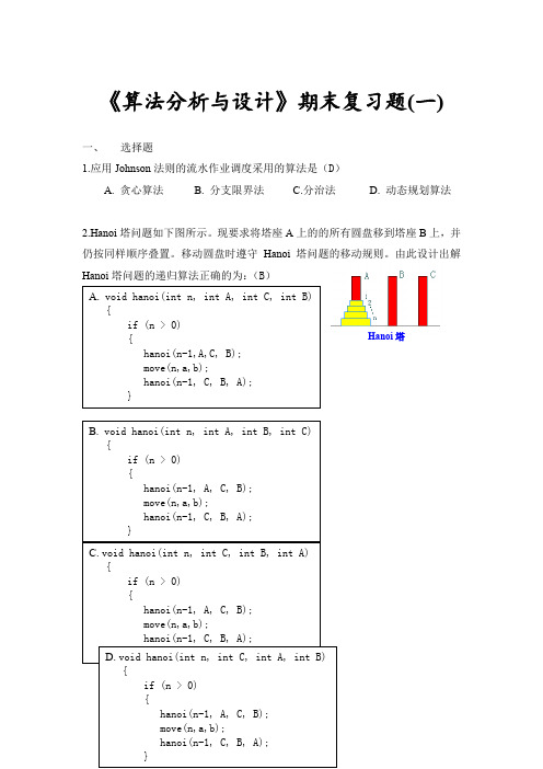
《算法分析与设计》期末复习题(一)一、选择题1.应用Johnson 法则的流水作业调度采用的算法是(D )A. 贪心算法B. 分支限界法C.分治法D. 动态规划算法2.Hanoi 塔问题如下图所示。
现要求将塔座A 上的的所有圆盘移到塔座B 上,并仍按同样顺序叠置。
移动圆盘时遵守Hanoi 塔问题的移动规则。
由此设计出解Hanoi 塔问题的递归算法正确的为:(B )Hanoi 塔3. 动态规划算法的基本要素为(C)A. 最优子结构性质与贪心选择性质B.重叠子问题性质与贪心选择性质C.最优子结构性质与重叠子问题性质D. 预排序与递归调用4. 算法分析中,记号O表示(B),记号Ω表示(A),记号Θ表示(D)。
A.渐进下界B.渐进上界C.非紧上界D.紧渐进界E.非紧下界5. 以下关于渐进记号的性质是正确的有:(A)A.f(n)(g(n)),g(n)(h(n))f(n)(h(n))=Θ=Θ⇒=ΘB. f(n)O(g(n)),g(n)O(h(n))h(n)O(f(n))==⇒=C. O(f(n))+O(g(n)) = O(min{f(n),g(n)})D. f(n)O(g(n))g(n)O(f(n))=⇔=6.能采用贪心算法求最优解的问题,一般具有的重要性质为:(A)A. 最优子结构性质与贪心选择性质B.重叠子问题性质与贪心选择性质C.最优子结构性质与重叠子问题性质D. 预排序与递归调用7. 回溯法在问题的解空间树中,按(D)策略,从根结点出发搜索解空间树。
A.广度优先B. 活结点优先 C.扩展结点优先 D. 深度优先8. 分支限界法在问题的解空间树中,按(A)策略,从根结点出发搜索解空间树。
A.广度优先B. 活结点优先 C.扩展结点优先 D. 深度优先9. 程序块(A)是回溯法中遍历排列树的算法框架程序。
A.B.C.D.10. 回溯法的效率不依赖于以下哪一个因素?(C )A.产生x[k]的时间;B.满足显约束的x[k]值的个数;C.问题的解空间的形式;D.计算上界函数bound的时间;E.满足约束函数和上界函数约束的所有x[k]的个数。
山东建筑大学计算机学院算法分析算法复习题(Yuconan翻译)
1.The O-notation provides an asymptotic upper bound. The Ω-notationprovides an asymptotic lower bound. The Θ-notation asymptoticallya function form above and below.2.To represent a heap as an array,the root of tree is A[1], and giventhe index i of a node, the indices of its parent Parent(i) { return ⎣i/2⎦; },left child, Left(i) { return 2*i; },right child, right(i) { return 2*i + 1; }.代表一个堆中的一个数组,树的根节点是A[1],并且给出一个节点i,那么该节点的父节点是左孩子右孩子3.Because the heap of n elements is a binary tree, the height of anynode is at most Θ(lg n).因为n个元素的堆是一个二叉树,任意节点的树高最多是4.In optimization problems, there can be many possible solutions. Eachsolution has a value, and we wish to find a solution with the optimal (minimum or maximum) value. We call such a solution an optimal solution to the problem.在最优化问题中,有很多可能的解,每个解都有一个值,我们希望找到一个最优解(最大或最小),我们称这个解为最优解问题。
山东建筑大学计算机学院算法分析第三部分复习
第三部分复习与作业(动态规划和贪心算法)1 Dynamic programming, like the divide-and-conquer method, solves problems by combining the solutions to subproblems. divide-and-conquer algorithms partitionthe problem into independent subproblems, solve the subproblems recursively, and then combine their solutions to solve the original problem. In contrast, dynamic programming is applicable when the subproblems are not independent, that is, when subproblems share subsubproblems.2 In optimization problems, there can be many possible solutions. Each solution has a value, and we wish to find a solution with the optimal (minimum or maximum) value. We call such a solution an optimal solution to the problem.3 optimal substructure if an optimal solution to the problem contains within it optimal solutions to subproblems.4 In dynamic programming, we build an optimal solution to the problem from optimal solutions to subproblems.5 When a recursive algorithm revisits the same problem over and over again, we say that the optimization problem has overlapping subproblems.6 A subsequence of X if there exists a strictly increasing sequence <i1,i2, ..., i k> of indices of X such that for all j = 1, 2, ..., k, we have x i j= z j .7 Let X = <x1, x2, ..., x m> and Y = <y1, y2, ..., y n> be sequences, and let Z = <z1, z2, ..., z k> be any LCS of X and Y.1. If x m = y n, then z k = x m = y n and Z k-1is an LCS of X m-1 and Y n-1.2. If x m ≠y n, then z k ≠x m implies that Z is an LCS of X m-1 and Y.3. If x m ≠y n, then z k ≠y n implies that Z is an LCS of X and Y n-1.8 A greedy algorithm always makes the choice that looks best at the moment. That is, it makes a locally optimal choice in the hope that this choice will lead to a globally optimal solution.9 The greedy-choice property and optimal sub-structure are the two key ingredients of greedy algorithm.10 greedy-choice property is a globally optimal solution can be arrived at by makinga locally optimal (greedy) choice.1 The Motors Corporation produces automobiles in a factory that has two assembly lines. An automobile chassis enters each assembly line, has parts added to it at a number of stations, and a finished auto exits at the end of the line. Each assembly line has n stations, numbered j = 1, 2, ..., n. We denote the j th station on line i (where i is 1 or 2) by S i,j. The j th station on line 1 (S1,j) performs the same function as the j th station on line2 (S2,j). The stations were built at different times and with different technologies, however, so that the time required at each station varies, even between stations at the same position on the two different lines. We denote the assembly time required at station S i,j by a i,j. a chassis enters station 1 of one of the assembly lines, and it progresses from each station to the next. There is also an entry time e i for the chassis to enter assembly line i and an exit time x i for the completed auto to exitassembly line i. The time to transfer a chassis away from assembly line i after having gone through station S i,j is t i,j, where i = 1, 2 and j = 1, 2, ..., n – 1. A manufacturing problem is to find the fastest way through a factory. Let f i[j] denote the fastest possible time to get a chassis from the starting point through station S i,j. Our ultimate goal is to determine the fastest time to get a chassis all the way through the factory, which we denote by f*. Please write its recursive formula and compute the fastest time and construct the fastest way through the factory of the instance.2 The matrix-chain multiplication problem can be stated as follows: given a chain<A1,A2,…,An>of matrices, where for i=1,2…,n, matrix A i has dimensionP i-1 P i, fully parenthesize the product A1,A2,…,A n in a way that minimizes the number of scalar multiplication. We pick as our subproblems the problems of determining the minimum cost of a parenthesization of A i A i+1 A j for 1 ≤i ≤j ≤n. Let m[i, j] be the minimum number of scalar multiplications needed to compute the matrix A i..j; for the full problem, the cost of a cheapest way to compute A1..n would thus be m[1, n]. Can you define m[i, j] recursively? Find an optimal parenthesization of a matrix-chain product whose sequence of dimensions is <2,1,3,2,4>3 In the longest-common-subsequence (LCS) problem, we are given two sequences X = <x1, x2, ...,x m> and Y = <y1, y2, ..., y n> and wish to find a maximum-length common subsequence of X and Y. Please write its recursive formula and determine an LSC of <1,0,0,1,0,1,0,1> and <0,1,0,1,1,0,1,1,0>.4 The 0–1 knapsack problem is posed as follows. A thief robbing a store finds n items; the i th item is worth v i dollars and weighs w i pounds, where v i and w i are integers. He wants to take as valuable a load as possible, but he can carry at most W pounds in his knapsack for some integer W. Which items should he take? This is called the 0–1 knapsack problem because each item must either be taken or left behind; the thief cannot take a fractional amount of an item or take an item more than once. In the fractional knapsack problem, the setup is the same, but the thief can take fractions of items, rather than having to make a binary (0–1) choice for each item. Can the above two problems is solved by greedy strategy? Why?(P382)5 What is an optimal Huffman code for the following set of frequencies, based on the6 numbers? a:45 b:13 c:12 d:16 e:9 f:5。
山东建筑大学计算机学院算法分析第二部分复习

True-false questions1 To represent a heap as an array,the root of tree is A[1], and given the index i of a node, the indices of its parent Parent(i) { return ⎣i/2⎦; },left child, Left(i) { return 2*i; },right child, right(i) { return 2*i + 1; }.2 min-Heaps satisfy the heap property: A[Parent(i)] ≥ A[i] for all nodes i > 1.3 Because the heap of n elements is a binary tree, the height of any node is at most Θ(lg n).4 for array of length n, all elements in range A[⎣n/2⎦ + 1 .. n] are heaps5 the running time of build a heap is O(n lg n).6 The tighter bound of the running time to build a max-heap from an unordered array in linear time.7 The call to BuildHeap() takes O(n) time, Each of the n - 1 calls to Heapify() takes O(lg n) time, Thus the total time taken by HeapSort() = O(n) + (n - 1) O(lg n)= O(n) + O(n lg n)= O(n lg n).8 A priority queue is a data structure for maintaining a set S of elements, each with an associated value or key.9 The running time of Quick Sort is O(n lg n) in the average case, and O(n2) in the worst case.10 Quick Sort is a divide-and-conquer algorithm. The array A[p..r] is partitioned into two non-empty subarrays A[p..q] and A[q+1..r], All elements in A[p..q] are less than all elements in A[q+1..r], the subarrays are recursively sorted by calls to quicksort.11 Quick sorts, unlike merge sorts, have no combining step: two subarrays form an already-sorted array.12 A decision tree represents the comparisons made by a comparison sort.13 The asymptotic height of any decision tree for sorting n elements is Ω(n lg n).14 The running time of Counting sort is O(n + k). But the running time of sorting is Ω(n lg n). So this is contradiction.15 The Counting sort is stable.16 The radix sort can be used on card sorting.17 In radix sort, Sort elements by digit starting with least significant, Use a stable sort (like counting sort) for each stage.18 In the selection problem, finding the i th smallest element of a set, there is a practical randomized algorithm with O(n) expected running time.19 In the selection problem,there is a algorithm of theoretical interest only with O(n) worst-case running time.1 Write the running time of the Heapify procedure with recurrences. Solve the recurrences with Master method.Heapify(A, i){l = Left(i); r = Right(i);if (l <= heap_size(A) && A[l] > A[i])largest = l;elselargest = i;if (r <= heap_size(A) && A[r] > A[largest])largest = r;if (largest != i)Swap(A, i, largest);Heapify(A, largest);}Fixing up relationships between i, l, and r takes Θ(1) timeIf the heap at i has n elements, how many elements can the subtrees at l or r have?Answer: 2n/3 (worst case: bottom row 1/2 full)So time taken by Heapify() is given byT(n)≤T(2n/3) + Θ(1)By case 2 of the master theorem is T(n)=O(lgn)2 proof: with the array representation for storing an n-element heap, the leaves are the nodes indexed by ⎣n/2⎦+1,⎣n/2⎦+2,…,n. (10 points)Because a leaf in a heap is a node that has no left son, so for the first leaf that has no children, 2i > n. That is, i = ⎣n/2⎦+1,⎣n/2⎦+2,…,n.3 Heapsort(A){BuildHeap(A);for (i = length(A) downto 2){Swap(A[1], A[i]);heap_size(A) -= 1;Heapify(A, 1);}}We know that the call to BuildHeap() takes O(n) time. Each of the n - 1 calls to Heapify() takes O(lg n) time. Thus the total time taken by HeapSort() = O(n) + (n - 1) O(lg n)= O(n) + O(n lg n)= O(n lg n)1 CountingSort(A, B, k)2 for i=1 to k3 C[i]= 0;4 for j=1 to n5 C[A[j]] += 1;6 for i=2 to k7 C[i] = C[i] + C[i-1];8 for j=n downto 19 B[C[A[j]]] = A[j];10 C[A[j]] -= 1;Analysze its running time.Selection problemRandomizedSelect(A, p, r, i)if (p == r) then return A[p];q = RandomizedPartition(A, p, r)k = q - p + 1;if (i == k) then return A[q]; // not in bookif (i < k) thenreturn RandomizedSelect(A, p, q-1, i);elsereturn RandomizedSelect(A, q+1, r, i-k);Write an algorithm of the selection problem that the worst-case running time is linear-time.1. Divide n elements into groups of 52. Find median of each group3. Use Select() recursively to find median x of the ⎣n/5⎦4. Partition the n elements around x. Let k = rank(x)5. if (i == k) then return xif(i < k) then use Select() recursively to find i th smallest element in first partitionelse (i > k) use Select() recursively to find (i-k)th smallest element in last partition T(n)=T(1/5n)+T(7/10n)+ Θ(n)。
算法设计与分析复习题目及答案.docx

算法设计与分析复习题目及答案.docx一。
选择题1、二分搜索算法是利用(A)实现的算法。
A、分治策略B、动态规划法C、贪心法D、回溯法2、下列不是动态规划算法基本步骤的是(B)。
A、找出最优解的性质B、构造最优解C、算出最优解D、定义最优解3、最大效益优先是(A)的一搜索方式。
A、分支界限法B、动态规划法C、贪心法D、回溯法4、在下列算法中有时找不到问题解的是(B)。
A、蒙特卡罗算法B、拉斯维加斯算法C、舍伍德算法D、数值概率算法5. 回溯法解旅行售货员问题时的解空间树是(B)。
A、子集树B、排列树C、深度优先生成树D、广度优先生成树6.下列算法常以自底向上的方式求解最优解的是(B)。
A、备忘录法B、动态规划法C、贪心法D、回溯法7、衡量一个算法好坏的标准是( C )。
A 运行速度快B 占用空间少C 时间复杂度低D 代码短8、以下不可以使用分治法求解的是( D )。
A 棋盘覆盖问题B 选择问题C 归并排序D 0/1 背包问题9. 实现循环赛日程表利用的算法是(A)。
A、分治策略B、动态规划法C、贪心法D、回溯法10、下列随机算法中运行时有时候成功有时候失败的是( C )A 数值概率算法B 舍伍德算法C 拉斯维加斯算法D 蒙特卡罗算法11.下面不是分支界限法搜索方式的是(DA、广度优先B、最小耗费优先C、最大效益优先12.下列算法常以深度优先方式系统搜索问题解的是(A、备忘录法B、动态规划法C、贪心法13.备忘录方法是那种算法的变形。
( B )A、分治法B、动态规划法C、贪心法14.哈弗曼编码的贪心算法所需的计算时间为(BnB、 O(nlogn )n )A、O( n2 )C、O(215.分支限界法解最大团问题时,活结点表的组织形式是(A、最小堆B、最大堆C、栈组)。
D、深度优先D)。
D、回溯法D、回溯法)。
D、 O( n)B)。
D 、数16.最长公共子序列算法利用的算法是(B)。
A、分支界限法B、动态规划法C、贪心法D、回溯法17.实现棋盘覆盖算法利用的算法是(A)。
- 1、下载文档前请自行甄别文档内容的完整性,平台不提供额外的编辑、内容补充、找答案等附加服务。
- 2、"仅部分预览"的文档,不可在线预览部分如存在完整性等问题,可反馈申请退款(可完整预览的文档不适用该条件!)。
- 3、如文档侵犯您的权益,请联系客服反馈,我们会尽快为您处理(人工客服工作时间:9:00-18:30)。
1.The O-notation provides an asymptotic upper bound. The Ω-notationprovides an asymptotic lower bound. The Θ-notation asymptoticallya function form above and below.2.To represent a heap as an array,the root of tree is A[1], and giventhe index i of a node, the indices of its parent Parent(i) { return ⎣i/2⎦; },left child, Left(i) { return 2*i; },right child, right(i) { return 2*i + 1; }.代表一个堆中的一个数组,树的根节点是A[1],并且给出一个节点i,那么该节点的父节点是左孩子右孩子3.Because the heap of n elements is a binary tree, the height of anynode is at most Θ(lg n).因为n个元素的堆是一个二叉树,任意节点的树高最多是4.In optimization problems, there can be many possible solutions. Eachsolution has a value, and we wish to find a solution with the optimal (minimum or maximum) value. We call such a solution an optimal solution to the problem.在最优化问题中,有很多可能的解,每个解都有一个值,我们希望找到一个最优解(最大或最小),我们称这个解为最优解问题。
5.optimal substructure if an optimal solution to the problem containswithin it optimal solutions to subproblems.最优子结构中问题的最优解,至少包含它的最优解的子问题。
6. A subsequence of X if there exists a strictly increasing sequence<i1,i2, ..., i k> of indices of X such that for all j = 1, 2, ..., k, we have x i j= z j .Let X = <x1, x2, ..., x m> and Y = <y1, y2, ..., y n> be sequences, and let Z = <z1, z2, ..., z k> be any LCS of X and Y.(1). If x m = y n, then z k = x m = y n and Z k-1 is an LCS of X m-1 and Y n-1.(2). If x m ≠ y n, then z k ≠ x m implies that Z is an LCS of X m-1 and Y.(3). If x m ≠ y n, then z k ≠ y n implies that Z is an LCS of X and Y n-1.7. A greedy algorithm always makes the choice that looks best at themoment. That is, it makes a locally optimal choice in the hope that this choice will lead to a globally optimal solution.贪心算法经常需要在某个时刻寻找最好的选择。
正因如此,它在当下找到希望中的最优选择,以便引导出一个全局的最优解。
8.The greedy-choice property and optimal sub-structure are the two keyingredients of greedy algorithm.贪心选择和最优子结构是贪心算法的两个重要组成部分。
9.When a recursive algorithm revisits the same problem over and overagain, we say that the optimization problem has overlappingsubproblems.当一个递归算法一遍一遍的遍历同一个问题时,我们说这个最优化问题是重叠子问题。
10.greedy-choice property is a globally optimal solution can be arrivedat by making a locally optimal (greedy) choice.贪心选择性质是一个全局的最优解,这个最优解可以做一个全局的最优选择。
11.An approach of Matrix multiplication can develope a Θ(V4)-timealgorithm for the all-pairs shortest-paths problem and then improve its running time to Θ(V3lg V).一个矩阵相乘问题的解决可以一个时间复杂度算法的所有路径的最短路径问题,改进后的时间复杂度是。
12.Floyd-Warshall algorithm, runs in Θ(V3) time to solve the all-pairsshortest-paths problem.FW算法在时间复杂度下可以解决最短路径问题。
13.The running time of Quick Sort is O(n2) in the worst case, and O(n lgn) in the average case.快速排序的平均时间复杂度是O(n lg n),最坏时间复杂度是O(n2)。
14.The MERGE(A,p,q,r) procedure in merge sort takes time Θ(n).MERGE在归并排序中所花费的时间是。
15.Given a weighted, directed graph G = (V, E) with source s and weightfunction w : E →R, the Bellman-Ford algorithm makes |V| - 1 passes over the edges of the graph.给一个带权重的有向图G = (V, E),权重关系w : E →R,则the Bellman-Ford算法需经过条边。
16.The Bellman-Ford algorithm runs in time O(V E).Bellman ford 算法的时间复杂度是。
17.A decision tree represents the comparisons made by a comparisonsort.The asymptotic height of any decision tree for sorting n elements is (n lg n).一个决策树代表一个比较类型,通过比较排序。
N个元素的任意决策树的渐进高度是。
True-false questions1.An algorithm is said to be correct if, for some input instance, it haltswith the correct output F如果给一个算法输入一些实例,并且它给力正确的输出,则认识这个算法是正确的。
2.Insertion sort always best merge sort F插入排序总是优越与归并排序。
3.Θ(n lg n) grows more slowly than Θ(n2). Therefore, merge sortasymptotically beats insertion sort in the worst case. TΘ(n lg n)4.Currently computers are fast and computer memory is very cheap, we haveno reason to study algorithms. F5.In RAM (Random-Access Machine) model, instructions are executed withconcurrent operations. F6.The running time of an algorithm on a particular input is the numberof primitive operations or “steps” executed. T7.Quick sorts, have no combining step: two subarrays form analready-sorted array. T8.The running time of Counting sort is O(n + k). But the running timeof sorting is (n lg n). So this is contradiction. F9.The Counting sort is stable. T10.In the selection problem,there is a algorithm of theoretical interestonly with O(n) worst-case running time. T11.Divide-and-conquer algorithms partition the problem into independentsubproblems, solve the subproblems recursively, and then combine their solutions to solve the original problem. In contrast, dynamicprogramming is applicable when the subproblems are not independent, that is, when subproblems share subsubproblems. T12.In dynamic programming, we build an optimal solution to the problemfrom optimal solutions to subproblems. T13.The best-case running time is the longest running time for any inputof size n. F14.When we analyze the running time of an algorithm, we actuallyinterested on the rate of growth (order of growth). T15.The dynamic programming approach means that it break the problem intoseveral subproblems that are similar to the original problem butsmaller in size, solve the subproblems recursively, and then combinethese solutions to create a solution to the original problem. T16.Insertion sort and merge sort both use divide-and-conquer approach.F17.Θ(g(n)) = { f (n) : there exist positive constants c1, c2, and n0 suchthat 0 ≤c1 g(n) ≤f (n) ≤c2 g(n) for all n ≥n0 }18.Min-Heaps satisfy the heap property: A[Parent(i)] ≥ A[i] forall nodes i > 1. F19.For array of length n, all elements in range A[⎣n/2⎦+ 1 .. n] are heaps.T20.The tighter bound of the running time to build a max-heap from anunordered array isn’t in linear time. F21.The call to BuildHeap() takes O(n) time, Each of the n - 1 calls toHeapify()takes O(lg n) time, Thus the total time taken by HeapSort()= O(n) + (n - 1) O(lg n)= O(n) + O(n lg n)= O(n lg n). T22.Quick Sort is a dynamic programming algorithm. The array A[p..r] ispartitioned into two non-empty subarrays A[p..q] and A[q+1..r], All elements in A[p..q] are less than all elements in A[q+1..r], the subarrays are recursively sorted by calls to quicksort. F 23.Assume that we have a connected, undirected graph G = (V, E) with aweight function w : E→R, and we wish to find a minimum spanning tree for G. Both Kruskal and Prim algorithms use a dynamic programming approach to the problem. F24.A cut (S, V - S) of an undirected graph G = (V, E) is a partition ofE. F25.An edge is a light edge crossing a cut if its weight is the maximumof any edge crossing the cut. F26.Kruskal's algorithm uses a disjoint-set data structure to maintainseveral disjoint sets of elements. T27.Optimal-substructure property is a hallmark of the applicability ofboth dynamic programming. T28.Dijkstra's algorithm is a dynamic programming algorithm. F29.Floyd-Warshall algorithm, which finds shortest paths between all pairsof vertices , is a greedy algorithm. F30.Given a weighted, directed graph G = (V, E) with weight function w :E →R, let p = <v1,v2,..., v k_>be a shortest path from vertex v1 tovertex v k and, for any i and j such that 1 ≤i ≤j ≤k, let p ij = <v i,v i+1,..., v j> be the subpath of p from vertex v i to vertex v j . Then,p ij is a shortest path from v i to v j. T31.Given a weighted, directed graph G = (V, E) with weight function w :E →R,If there is a negative-weight cycle on some path from s to v ,there exists a shortest-path from s to v. F32.Since any acyclic path in a graph G = (V, E) contains at most |V|distinct vertices, it also contains at most |V| - 1 edges. Thus, wecan restrict our attention to shortest paths of at most |V| - 1 edges.T33.The process of relaxing an edge (u, v) tests whether we can improvethe shortest path to v found so far by going through u. T34.In Dijkstra's algorithm and the shortest-paths algorithm for directedacyclic graphs, each edge is relaxed exactly once. In the Bellman-Fordalgorithm, each edge is also relaxed exactly once . F35.The Bellman-Ford algorithm solves the single-source shortest-pathsproblem in the general case in which edge weights must be negative.F36.Given a weighted, directed graph G = (V, E) with source s and weightfunction w : E →R, the Bellman-Ford algorithm can not return aBoolean value indicating whether or not there is a negative-weightcycle that is reachable from the source. F37.Given a weighted, directed graph G = (V, E) with source s and weightfunction w : E →R, for the Bellman-Ford algorithm, if there is sucha cycle, the algorithm indicates that no solution exists. If there isno such cycle, the algorithm produces the shortest paths and their weights. F38.Dijkstra's algorithm solves the single-source shortest-paths problemon a weighted, directed graph G = (V, E) for the case in which all edge weights are negative. F39.Dijkstra's algorithm solves the single-source shortest-paths problemon a weighted, directed graph G = (V, E) for the case in which all edge weights are nonnegative. Bellman-Ford algorithm solves thesingle-source shortest-paths problem on a weighted, directed graph G = (V, E), the running time of Dijkstra's algorithm is lower than that of the Bellman-Ford algorithm. T40.The steps for developing a dynamic-programming algorithm:1.Characterize the structure of an optimal solution. 2. Recursively define the value of an optimal solution. 3. Compute the value of an optimal solution in a bottom-up fashion. 4. Construct an optimal solution from computed information. T三 Each of n input elements is an integer in the range 0 to k, Design a linear running time algorithm to sort n elements.四Design a expected linear running time algorithm to find the i th smallestelement of n elements using divide and conquer strategy.五Write the INSERT-SORT procedure to sort into non-decreasing order. Analyze the running time of it with RAM Model. What ’s the best-case running time, the worst-case running time and average case running time. Write the MERGE-SORT procedure to sort into non-decreasing order. Give the recurrence for the worst-case running time T(n) of Merge sort and find the solution to the recurrence.六 What is an optimal Huffman code for the following set of frequencies, <a:45, b:13, c:12,d:16,e:9,f:5>七 The traveling-salesman problem (TSP): in the traveling-salesman problem, we are given a complete undirected graph G=(V,E) that has a nonnegative integer cost c(u,v) associated with each edge (u,v)∈E , and we must find a tour of G with minimum cost. The following is an instance TSP. Please compute a tour with minimum cost with greedy algorithm. ∞∞∞∞∞69326911699252312514216214八Given items of different values and weights, find the most valuable set of items that fit in a knapsack of fixed weight C .For an instance of knapsack problem, n =8, C =110,value V ={11,21,31,33,43,53,55,65} weight W ={1,11,21,23,33,43,45,55}. Use greedy algorithms to solve knapsackproblem.九Use dynamic programming to solve Assembly-line scheduling problem: A Motors Corporation produces automobiles that has two assembly lines, numbered i=1,2. Each line has n stations, numbered j=1,2…n. We denote the j th station on line i by S ij. The following figure is an instance of the assembly-line problem with costs entry time e i, exit time x i, the assembly time required at station S ij by a ij, the time to transfer a chassis away from assembly line I after having gone through station S ij is t ij. Please compute the fastest time and construct the fastest way through the factory of the instance.十. The matrix-chain multiplication problem can be stated as follows: given a chain <A1,A2,…,An>of matrices, where for i=1,2…,n, matrix A i has dimensionP i-1 P i, fully parenthesize the product A1,A2,…,A n in a way that minimizes the number of scalar multiplication. We pick as our subproblems the problems of determining the minimum cost of a parenthesization of A i A i+1 A j for 1 ≤i ≤j ≤n. Let m[i, j] be the minimum number of scalar multiplications needed to compute the matrix A i..j; for the full problem, the cost of a cheapest way to compute A1..n would thus be m[1, n]. Can you define m[i, j] recursively? Find an optimal parenthesization of a matrix-chain product whose sequence of dimensions is <4,3,5,2,3>十一 In the longest-common-subsequence (LCS) problem, we are given two sequences X = <x1, x2, ...,xm> and Y = <y1, y2, ..., yn> and wish to find a maximum-length common subsequence of X and Y.Please write its recursive formula and determine an LSC of Sequence S1=ACTGATCG and sequence S2=CATGC. Please fill in the blanks in the table below.C A T G C十二 Proof: Any comparison sort algorithm requires Ω(nlgn) comparisons in the worst case.How many leaves does the tree have? (叶节点的数目)–At least n! (each of the n!permutations if the input appears as some leaf) ⇒n! ≤l(至少n! 个,排列)–At most 2hleaves (引理,至多2h个)⇒n! ≤l ≤2h⇒h ≥lg(n!) = Ω(nlgn)十三Proof: Subpaths of shortest paths are shortest paths.Given a weighted, directed graph G = (V, E) with weight function w : E → R, let p =<v1,v2,..., v k> be a shortest path from vertex v1to vertex v k and, for any i and j such that 1 ≤i ≤j ≤k, let p ij= <v i, v i+1,..., v j>be the subpath of p from vertex v i to vertex v j . Then, p ij is a shortest path from v i to v j.十四Proof : The worst case running time of quicksort is Θ(n2)十五Compute shortest paths with matrix multiplication and the Floyd-Warshall algorithm for the following graph.十六 Write the MAX-Heapify() procedure to for manipulating max-heaps. And analyze the running time of MAX-Heapify().三(10分)1 CountingSort(A, B, k)2 for i=1 to k3 C[i]= 0;4 for j=1 to n5 C[A[j]] += 1;6 for i=2 to k7 C[i] = C[i] + C[i-1];8 for j=n downto 19 B[C[A[j]]] = A[j];10 C[A[j]] -= 1;四算法描述3分The best-case running time is T(n) = c1n + c2(n - 1) + c4(n - 1) + c5(n - 1) + c8(n - 1)= (c1+ c2+ c4+ c5+ c8)n - (c2+ c4+ c5 + c8). This running time can be expressed as an + b for constants a and b that depend on the statement costs c i; it is thus a linear function of n.This worst-case running time can be expressed as an2+ bn + c for constants a, b, and c that again depend on the statement costs c i; it is thus a quadratic function of n.分析2分算法描述2分Θ(1) if n = 1T(n) =2T(n/2) + Θ(n) if n > 1.递归方程和求解3分五7 RAND-SELECT(A, p, r, i) (5分)if p = r then return A[p]q ← RAND-PARTITION(A, p, r)k ← q – p + 1if i = k then return A[q]if i < kthen return RAND-SELECT(A, p, q – 1, i )else return RAND-SELECT(A, q + 1, r, i – k )Randomized RANDOMIZED-PARTITION(A; p; r) (5分) { i ←RANDOM(p, r)exchange A[r] ← A[i]return PARTITION(A; p; r)}PARTITION(A; p; r){ x← A[r]i ←p-1for j ← p to r-1do if A[j] ≤ xthen i ←i+1exchange A[i] ↔A[j]exchange A[i+1] ↔ A[r]return i+1}六首先画出它对应的图,加上标号,假设从1出发,每次贪心选择一个权重最小的顶点作为下一个要去的城市。