数字图像处理 Matlab 退化模型示例(example0507)
用matlab实现数字图像处理几个简单例子

实验报告实验一图像的傅里叶变换(旋转性质)实验二图像的代数运算实验三filter2实现均值滤波实验四图像的缩放朱锦璐04085122实验一图像的傅里叶变换(旋转性质)一、实验内容对图(1.1)的图像做旋转,观察原图的傅里叶频谱和旋转后的傅里叶频谱的对应关系。
图(1.1)二、实验原理首先借助极坐标变换x=rcosθ,y=rsinθ,u=wcosϕ,v=wsinϕ,,将f(x,y)和F(u,v)转换为f(r,θ)和F(w,ϕ).f(x,y) <=> F(u,v)f(rcosθ,rsinθ)<=> F(wcosϕ,wsinϕ)经过变换得f( r,θ+θ。
)<=>F(w,ϕ+θ。
)上式表明,对f(x,y)旋转一个角度θ。
对应于将其傅里叶变换F(u,v)也旋转相同的角度θ。
F(u,v)到f(x,y)也是一样。
三、实验方法及程序选取一幅图像,进行离散傅里叶变换,在对其进行一定角度的旋转,进行离散傅里叶变换。
>> I=zeros(256,256); %构造原始图像I(88:168,120:136)=1; %图像范围256*256,前一值是纵向比,后一值是横向比figure(1);imshow(I); %求原始图像的傅里叶频谱J=fft2(I);F=abs(J);J1=fftshift(F);figure(2)imshow(J1,[5 50])J=imrotate(I,45,'bilinear','crop'); %将图像逆时针旋转45°figure(3);imshow(J) %求旋转后的图像的傅里叶频谱J1=fft2(J);F=abs(J1);J2=fftshift(F);figure(4)imshow(J2,[5 50])四、实验结果与分析实验结果如下图所示(1.2)原图像(1.3)傅里叶频谱(1.4)旋转45°后的图像(1.5)旋转后的傅里叶频谱以下为放大的图(1.6)原图像(1.7)傅里叶频谱(1.8)旋转45°后的图像(1.9)旋转后的傅里叶频谱由实验结果可知1、从旋转性质来考虑,图(1.8)是图(1.6)逆时针旋转45°后的图像,对比图(1.7)和图(1.9)可知,频域图像也逆时针旋转了45°2、从尺寸变换性质来考虑,如图(1.6)和图(1.7)、图(1.8)和图(1.9)可知,原图像和其傅里叶变换后的图像角度相差90°,由此可知,时域中的信号被压缩,到频域中的信号就被拉伸。
Matlab中的模糊图像处理和图像模糊恢复技术
Matlab中的模糊图像处理和图像模糊恢复技术随着数字图像的广泛应用和发展,图像模糊成为一个重要的问题。
由于摄像器材或传输媒介等方面的限制,图像的清晰度可能受到一定程度的影响,导致图像模糊。
在实际应用中,图像的模糊问题会给图像解析、目标跟踪、计算机视觉等许多领域带来困扰。
为了改善模糊图像的质量,并解决图像模糊问题,Matlab提供了一系列的模糊图像处理和图像模糊恢复技术。
一、图像模糊的产生原因图像模糊一般是由光学系统的缺陷、运动物体、相机抖动等因素引起的。
光学系统的缺陷包括镜头的失真、散射、衍射等;运动物体指的是图像中的物体在拍摄过程中出现运动造成模糊;相机抖动是由于相机本身的不稳定性或者手持摄影造成的。
二、模糊图像处理的方法1.滤波方法滤波方法是最基本也是最常用的图像模糊处理方法。
在Matlab中,可以使用各种滤波器对图像进行处理,例如平滑滤波、高斯滤波、中值滤波等。
这些滤波器可以消除图像中的高频噪声,同时也会导致图像的模糊。
2.图像退化模型图像退化模型是描述图像模糊过程的数学模型。
常见的图像退化模型有运动模糊模型、模糊核模型等。
通过了解图像退化模型的特性,可以更准确地恢复图像的清晰度。
在Matlab中,可以根据图像退化模型进行图像恢复的研究和实现。
3.频域方法频域方法是一种基于图像频谱的模糊图像处理方法。
通过对图像进行傅里叶变换,可以将图像从空间域转换到频率域,然后在频率域进行处理,最后再进行逆傅里叶变换得到恢复后的图像。
在Matlab中,可以利用fft2函数进行傅里叶变换和逆傅里叶变换,实现频域方法对图像的处理。
三、图像模糊恢复技术1.盲去卷积算法盲去卷积算法是一种不需要知道图像退化模型的图像恢复方法。
通过对模糊图像进行去卷积处理,可以尽可能地恢复图像的清晰度。
在Matlab中,可以使用盲去卷积相关的函数和工具箱实现图像模糊恢复。
2.基于深度学习的图像超分辨率重建技术深度学习技术如今在计算机视觉领域取得了巨大的成功。
根据运动模糊的退化模型编写matlab函数
为了编写一个MATLAB函数来模拟运动模糊的退化模型,我们需要首先明确这个模型的数学描述。
通常,运动模糊可以被视为一种空间频率的衰减,其中高频分量(即,运动部分)比低频分量(即,静止部分)更快地衰减。
这可以通过将模糊核看作是一个函数来表示,这个函数随着距离的增加而减小。
下面是一个简单的例子,假设我们有一个高斯模糊核(也就是理想的运动模糊),并使用简单的空间频率衰减模型来模拟退化过程。
在这个模型中,我们假设模糊核的衰减速度是恒定的,并且衰减到零的时间与距离的平方成正比。
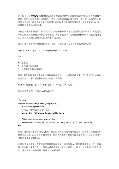
首先,我们需要定义模糊核的函数,这是一个在距离为x处具有高斯形状的函数:f(x) = 1 / (sqrt(2 * pi) * σ* x) * exp(- (x - v)2 / (2 * σ2))其中:* x 是距离* v 是模糊中心的速度* σ是模糊核的标准偏差然后,我们可以使用这个函数来模拟模糊核在经过一定时间后的退化过程。
我们假设衰减速度是恒定的,那么模糊核在经过t时间后将变为:f(x, t) = 1 / (sqrt(2 * pi) * σ* t) * exp(- (x - v * t)2 / (2 * σ2))这可以被表示为一个新的MATLAB函数:```matlabfunction [deconvolved] = deblur_simple(blur, t)% Define blur parametersv = 0.1; % Velocity of blur centersigma = 0.5; % Standard deviation of blur kernel% Compute deconvolved image at time tdeconvolved = 1 ./ (sqrt(2 * pi) * sigma * t) .* exp(- ((x - v * t) .^ 2) ./ (2 * sigma^2));end```注意,这只是一个非常简化的模型,真实世界的运动模糊通常更复杂,需要更高级的模型和算法来进行退化。
Matlab中的图像配准与对齐方法

Matlab中的图像配准与对齐方法图像配准与对齐是数字图像处理中的重要步骤,能够将多幅图像对齐到同一坐标系,实现图像的比较、特征提取和分析。
Matlab作为一种强大的计算工具和编程语言,提供了多种图像配准与对齐方法的函数和工具箱,方便用户进行图像处理和分析。
本文将介绍Matlab中的一些常用的图像配准与对齐方法,包括特征点配准、基于亮度的配准和图像退化模型配准。
一、特征点配准特征点配准是一种常用的图像配准方法,通过在两幅图像中提取出一些具有显著特征的点,并将这些点匹配起来,从而实现图像的对准。
Matlab提供了SURF (Speeded Up Robust Features)算法和SIFT(Scale-Invariant Feature Transform)算法用于特征点的提取和匹配。
用户可以使用Matlab的Image Processing Toolbox中的相关函数,在两幅图像中提取出SURF或SIFT特征点,并使用Matlab的vision.PointTracker对象进行特征点的匹配和跟踪。
通过特征点的匹配,可以获取两幅图像之间的变换矩阵,进而实现图像的配准和对齐。
二、基于亮度的配准基于亮度的配准方法是一种利用图像亮度信息进行对齐的方法,其原理是通过优化亮度的判断标准,使两幅图像的亮度分布尽量一致,从而实现图像的对齐。
Matlab提供了基于亮度的配准算法,用户可以使用Matlab的imregcorr函数进行基于亮度的图像配准。
该函数可以计算两幅图像之间的亮度相关性,并找到亮度最大的对齐方式。
通过该算法,用户可以快速实现对齐图像的配准。
三、图像退化模型配准图像退化模型配准是一种利用具有退化模型的图像进行对齐的方法,其原理是先对待配准图像进行退化处理,再与目标图像进行比较,从而找到最佳的配准方式。
Matlab提供了图像退化模型配准的函数和工具箱,用户可以使用Matlab的ImageProcessing Toolbox中的相关函数,对图像进行退化处理和模型建立,并通过最小二乘法求解配准参数。
数字图像处理实验三:图像的复原
南京工程学院通信工程学院实验报告课程名称数字图像处理C实验项目名称实验三图像的复原实验班级算通111 学生姓名夏婷学号 208110408 实验时间 2014年5月5日实验地点信息楼C322实验成绩评定指导教师签名年月日实验三、图像的恢复一、实验类型:验证性实验二、实验目的1. 掌握退化模型的建立方法。
2. 掌握图像恢复的基本原理。
三、实验设备:安装有MATLAB 软件的计算机四、实验原理一幅退化的图像可以近似地用方程g=Hf+n 表示,其中g 为图像,H为变形算子,又称为点扩散函数(PSF ),f 为原始的真实图像,n 为附加噪声,它在图像捕获过程中产生并且使图像质量变坏。
其中,PSF 是一个很重要的因素,它的值直接影响到恢复后图像的质量。
I=imread(‘peppers.png’);I=I(60+[1:256],222+[1:256],:);figure;imshow(I);LEN=31;THETA=11;PSF=fspecial(‘motion’,LEN,THETA);Blurred=imfilter(I,PSF,’circular’,’conv’);figure;imshow(Blurred);MATLAB 工具箱中有4 个图像恢复函数,如表3-1 所示。
这4 个函数都以一个PSF 和模糊图像作为主要变量。
deconvwnr 函数使用维纳滤波对图像恢复,求取最小二乘解,deconvreg 函数实现约束去卷积,求取有约束的最小二乘解,可以设置对输出图像的约束。
deconvlucy 函数实现了一个加速衰减的Lucy-Richardson 算法。
该函数采用优化技术和泊松统计量进行多次迭代。
使用该函数,不需要提供有关模糊图像中附加噪声的信息。
deconvblind 函数使用的是盲去卷积算法,它在不知道PSF 的情况下进行恢复。
调用deconvblind 函数时,将PSF 的初值作为一个变量进行传递。
matlab图像处理基础实例
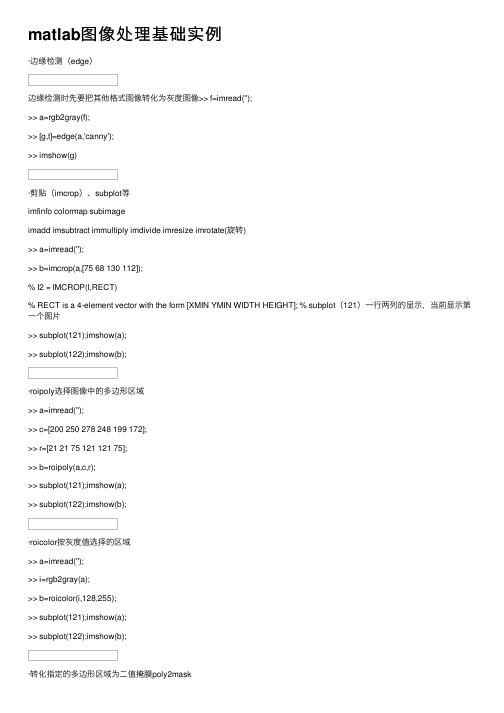
matlab图像处理基础实例·边缘检测(edge)边缘检测时先要把其他格式图像转化为灰度图像>> f=imread('');>> a=rgb2gray(f);>> [g,t]=edge(a,'canny');>> imshow(g)·剪贴(imcrop)、subplot等imfinfo colormap subimageimadd imsubtract immultiply imdivide imresize imrotate(旋转)>> a=imread('');>> b=imcrop(a,[75 68 130 112]);% I2 = IMCROP(I,RECT)% RECT is a 4-element vector with the form [XMIN YMIN WIDTH HEIGHT]; % subplot(121)⼀⾏两列的显⽰,当前显⽰第⼀个图⽚>> subplot(121);imshow(a);>> subplot(122);imshow(b);·roipoly选择图像中的多边形区域>> a=imread('');>> c=[200 250 278 248 199 172];>> r=[21 21 75 121 121 75];>> b=roipoly(a,c,r);>> subplot(121);imshow(a);>> subplot(122);imshow(b);·roicolor按灰度值选择的区域>> a=imread('');>> i=rgb2gray(a);>> b=roicolor(i,128,255);>> subplot(121);imshow(a);>> subplot(122);imshow(b);·转化指定的多边形区域为⼆值掩膜poly2mask>> x=[63 186 54 190 63];>> y=[60 60 209 204 60];>> b=poly2mask(x,y,256,256); >> imshow(b);>> holdCurrent plot held>> plot(x,y,'b','LineWidth',2)·roifilt2区域滤波a=imread('');i=rgb2gray(a);c=[200 250 278 248 199 172];r=[21 21 75 121 121 75];b=roipoly(i,c,r);h=fspecial('unsharp');j=roifilt2(h,i,b);subplot(121),imshow(i);subplot(122),imshow(j);·roifill区域填充>> a=imread('');>> i=rgb2gray(a);>> c=[200 250 278 248 199 172]; >> r=[21 21 75 121 121 75]; >> j=roifill(i,c,r); >> subplot(211);imshow(i);>> subplot(212);imshow(j);·FFT变换f=zeros(100,100);f(20:70,40:60)=1;imshow(f);F=fft2(f);F2=log(abs(F));imshow(F2),colorbar·补零操作和改变图像的显⽰象限f=zeros(100,100);f(20:70,40:60)=1;subplot(121);imshow(f);F=fft2(f,256,256);F2=fftshift(F);subplot(122);imshow(log(abs(F2)))·离散余弦变换(dct)>> a=imread('');>> i=rgb2gray(a);>> j=dct2(i);>> subplot(131);imshow(log(abs(j))),colorbar >> j(abs(j)<10)=0;>> k=idct2(j);>> subplot(132);imshow(i);>> subplot(133);imshow(k,[0,255]);info=imfinfo('')%显⽰图像信息·edge提取图像的边缘canny prewitt sobelradon函数⽤来计算指定⽅向上图像矩阵的投影>> a=imread('');>> i=rgb2gray(a);>> b=edge(i);>> theta=0:179;>> [r,xp]=radon(b,theta);>> figure,imagesc(theta,xp,r);colormap(hot); >> xlabel('\theta(degrees)'); >> ylabel('x\prime');>> title('r_{\theta}(x\prime)');>> colorbar·filter2均值滤波>> a=imread('');>> i=rgb2gray(a);>> imshow(i)>> k1=filter2(fspecial('average',3),i)/255;%3*3 >> k2=filter2(fspecial('average',5),i)/255;%5*5 >> k3=filter2(fspecial('average',7),i)/255;%7*7 >> figure,imshow(k1)>> figure,imshow(k2)>> figure,imshow(k3)wiener2滤波eg:k=wiener(I,[3,3]))medfilt2中值滤波同上deconvwnr维纳滤波马赫带效应(同等差⾊带条)·减采样>> a=imread('');>> b=rgb2gray(a);>> [wid,hei]=size(b);>> quarting=zeros(wid/2+1,hei/2+1); >> i1=1;j1=1;>> for i=1:2:widfor j=1:2:heiquarting(i1,j1)=b(i,j);j1=j1+1;endi1=i1+1;j1=1;end>> figure>> imshow(uint8(quarting))>> title('4倍减采样')>> quarting=zeros(wid/4+1,hei/4+1); i1=1;j1=1;for i=1:4:widfor j=1:4:heiquarting(i1,j1)=b(i,j);j1=j1+1;endi1=i1+1;j1=1;end>> figure,imshow(uint8(quarting)); title('16倍减采样')结论:在采⽤不同的减采样过程中,其图像的清晰度和尺⼨均发⽣了变化灰度级转化>> a=imread('');>> b=rgb2gray(a);>> figure;imshow(b)>> [wid,hei]=size(b);>> img2=zeros(wid,hei);>> for i=1:widfor j=1:heiimg2(i,j)=floor(b(i,j)/128);endend>> figure;imshow(uint8(img2),[0,2]) %2级灰度图像图像的基本运算>> i=imread('');>> figure;subplot(231);imshow(i);>> title('原图');>> j=imadjust(i,[.3;.6],[.1 .9]);%Adjust image intensity values or colormap图像灰度值或colormap调整% J = IMADJUST(I,[LOW_IN; HIGH_IN],[LOW_OUT; HIGH_OUT])>> subplot(232);imshow(j);title('线性扩展');>> i1=double(i);i2=i1/255;c=2;k=c*log(1+i2);>> subplot(233);imshow(k);>> title('⾮线性扩展');>> m=255-i;>> subplot(234);imshow(m)>> title('灰度倒置')>> n1=im2bw(i,.4);n2=im2bw(i,.7);>> subplot(235);imshow(n1);title('⼆值化阈值')>> subplot(236);imshow(n2);title('⼆值化阈值')图像的代数运算加。
数字图像处理ch01(MATLAB)-课件
2024/10/12
第一章 绪论
17
2024/10/12
第一章 绪论
18
2024/10/12
第一章 绪论
19
2024/10/12
第一章 绪论
20
<2>几何处理
放大、缩小、旋转,配准,几何校正,面积、周长计算。
请计算台湾的陆地面积
2024/10/12
第一章 绪论
21
<3>图象复原
由图象的退化模型,求出原始图象
图像处理是指按照一定的目标,用一系列的操 作来“改造”图像的方法.
2024/10/12
第一章 绪论
7
➢图象处理技术的分类(从方法上进行分类)[2]
1.模拟图象处理(光学图像处理等)
用光学、电子等方法对模拟信号组成的图像,用光学器 件、电子器件进行光学变换等处理得到所需结果(哈哈 镜、望远镜,放大镜,电视等).
2024/10/12
第一章 绪论
22
<4>图象重建[3]
[3]此图像来自罗立民,脑成像,
2024/10/12
第一章 绪论
23
/zhlshb/ct/lx.htm
2024/10/12
第一章 绪论
图形用户界面,动画,网页制作等
2024/10/12象处理的基本概念,和基 本问题,以及一些典型的应用。
2024/10/12
第一章 绪论
33
提问
摄像头(机),扫描仪,CT成像装置,其他图象成像装置
2)图象的存储
各种图象存储压缩格式(JPEG,MPEG等),海量图象数据库技术
3)图象的传输
内部传输(DirectMemoryAccess),外部传输(主要是网络)
第四章 图像复原-第2讲图像退化的数学模型

大小为M×N的周期数据,其中M≥A+C-1,N≥B+D-1。
fe
x,
y
f
x, 0
y
0 ≤ x ≤ A 1和0 ≤ y ≤ B 1 A ≤ x ≤ M 1或B ≤ y ≤ N 1
he
x,
y
h
x, 0
y
ne
x,
y
n
x, 0
y
0 ≤ x ≤ C 1和0 ≤ y ≤ D 1 C ≤ x ≤ M 1或D ≤ y ≤ N 1
为此就要采取其他有效策略,方法之一是利用矩阵的 特殊性质,将其对角化;更有效方法就是利用傅里叶变换 卷积定理在频域中处理;实际上对角化的结果与傅里叶变 换的结果是统一的。
9
4.2 图像退化的数学模型
g(x,y)=f(x,y)*h(x,y)+n(x,y) G (u,v)= H(u,v)F(u,v)+N(u,v) 注意事项:
F (u, v)
T 0
exp
j2 (ux0(t)dt
F(u,v)H (u,v)
11
4.2 图像退化的数学模型
H (u, v)
T 0
exp
j
2
(ux0
(t
)
dt
若x0(t)=at/T, 则 H (u, v) T sin(ua)e jua ua
若x0(t)=at/T, y0(t)= bt/T, 则
10
4.2 图像退化的数学模型
(6)常见退化模型
1)运动模糊退化模型 原因、类型:平移、旋转、匀速、变速等。这里讨论匀速 直线运动。设T为快门时间,x0(t)为位移的x分量。
- 1、下载文档前请自行甄别文档内容的完整性,平台不提供额外的编辑、内容补充、找答案等附加服务。
- 2、"仅部分预览"的文档,不可在线预览部分如存在完整性等问题,可反馈申请退款(可完整预览的文档不适用该条件!)。
- 3、如文档侵犯您的权益,请联系客服反馈,我们会尽快为您处理(人工客服工作时间:9:00-18:30)。
>> f=checkerboard (8);>> imshow (f)>> PSF=fspecial ('motion', 7, 45);>> gb = imfilter( f, PSF, ' circular' );>> noise = imnoise(zeros(size(f)),'gaussian',0,0.001);>> g = gb + noise;F GbNoise G% 可用MATLAB的fspecial建立PSF模型% PSF = fspecial(‘motion’,len,theta)% Len 移动的像素数% Theta运动方向(逆时针)>> help fspecialFSPECIAL Create predefined 2-D filters.H = FSPECIAL (TYPE) creates a two-dimensional filter H of the specified type. Possible values for TYPE are:'average' averaging filter'disk' circular averaging filter'gaussian' Gaussian lowpass filter'laplacian' filter approximating the 2-D Laplacian operator'log' Laplacian of Gaussian filter'motion' motion filter'prewitt' Prewitt horizontal edge-emphasizing filter'sobel' Sobel horizontal edge-emphasizing filter'unsharp' unsharp contrast enhancement filterDepending on TYPE, FSPECIAL may take additional parameters which you can supply. These parameters all have default values.H = FSPECIAL ('average', HSIZE) returns an averaging filter H of size HSIZE. HSIZE can be a vector specifying the number of rows and columns in H or a scalar, in which case H is a square matrix. The default HSIZE is [3 3].H = FSPECIAL('disk',RADIUS) returns a circular averaging filter (pillbox) within the square matrix of side 2*RADIUS+1. The default RADIUS is 5.H = FSPECIAL('gaussian',HSIZE,SIGMA) returns a rotationally symmetric Gaussian lowpass filter of size HSIZE with standard deviation SIGMA (positive). HSIZE can be a vector specifying the number of rows and columns in H or a scalar, in which case H is a square matrix. The default HSIZE is [3 3], the default SIGMA is 0.5.H = FSPECIAL('laplacian',ALPHA) returns a 3-by-3 filter approximating the shape of the two-dimensional Laplacian operator. The parameter ALPHA controls the shape of the Laplacian and must be in the range 0.0 to 1.0.The default ALPHA is 0.2.H = FSPECIAL('log',HSIZE,SIGMA) returns a rotationally symmetric Laplacian of Gaussian filter of size HSIZE with standard deviation SIGMA (positive). HSIZE can be a vector specifying the number of rows and columns in H or a scalar, in which case H is a square matrix. The default HSIZE is [5 5], the default SIGMA is 0.5.H = FSPECIAL('motion',LEN,THETA) returns a filter to approximate, once convolved with an image, the linear motion of a camera by LEN pixels, with an angle of THETA degrees in a counter-clockwise direction. The filter becomes a vector for horizontal and vertical motions. The default LEN is 9, the default THETA is 0, which corresponds to a horizontal motion of 9 pixels.H = FSPECIAL('prewitt') returns 3-by-3 filter that emphasizes horizontal edges by approximating a vertical gradient. If you need to emphasize vertical edges, transpose the filter H: H'.[1 1 1;0 0 0;-1 -1 -1].H = FSPECIAL('sobel') returns 3-by-3 filter that emphasizes horizontal edges utilizing the smoothing effect by approximating a vertical gradient. If you need to emphasize vertical edges, transpose the filter H: H'.[1 2 1;0 0 0;-1 -2 -1].H = FSPECIAL('unsharp',ALPHA) returns a 3-by-3 unsharp contrast enhancement filter. FSPECIAL creates the unsharp filter from the negative of the Laplacian filter with parameter ALPHA. ALPHA controls the shape of the Laplacian and must be in the range 0.0 to 1.0. The default ALPHA is 0.2.Class Support-------------H is of class double.Example-------I = imread('cameraman.tif');subplot(2,2,1);imshow(I);title('Original Image');H = fspecial('motion',20,45);MotionBlur = imfilter(I,H,'replicate');subplot(2,2,2);imshow(MotionBlur);title('Motion Blurred Image');H = fspecial('disk',10);blurred = imfilter(I,H,'replicate');subplot(2,2,3);imshow(blurred);title('Blurred Image');H = fspecial('unsharp');sharpened = imfilter(I,H,'replicate');subplot(2,2,4);imshow(sharpened);title('Sharpened Image');See also conv2, edge, filter2, fsamp2, fwind1, fwind2, imfilter.Reference page in Help browser doc fspecial>> help imfilter IMFILTER N-D filtering of multidimensional images.B = IMFILTER(A,H) filters the multidimensional array A with the multidimensional filter H. A can be logical or it can be a nonsparse numeric array of any class and dimension. The result, B, has the same size and class as A.Each element of the output, B, is computed using double-precision floating point. If A is an integer or logical array, then output elements that exceed the range of the given type are truncated, and fractional values are rounded.B = IMFILTER(A,H,OPTION1,OPTION2,...) performs multidimensional filtering according to the specified options. Option arguments can have the following values:- Boundary optionsX Input array values outside the bounds of the arrayare implicitly assumed to have the value X. When noboundary option is specified, IMFILTER uses X = 0.'symmetric' Input array values outside the bounds of the arrayare computed by mirror-reflecting the array acrossthe array border.'replicate' Input array values outside the bounds of the arrayare assumed to equal the nearest array bordervalue.'circular' Input array values outside the bounds of the arrayare computed by implicitly assuming the input arrayis periodic.- Output size options(Output size options for IMFILTER are analogous to the SHAPE option in the functions CONV2 and FILTER2.)'same' The output array is the same size as the inputarray. This is the default behavior when no outputsize options are specified.'full' The output array is the full filtered result, and sois larger than the input array.- Correlation and convolution'corr' IMFILTER performs multidimensional filtering usingcorrelation, which is the same way that FILTER2performs filtering. When no correlation orconvolution option is specified, IMFILTER usescorrelation.'conv' IMFILTER performs multidimensional filtering usingconvolution.Notes-----On some Intel Architecture processors, IMFILTER can take advantage of the Intel Performance Primitives Library (IPPL), thus accelerating its execution time. IPPL is activated only if A and H are both two dimensional and A is uint8, int16 or single.When IPPL is used, imfilter has different rounding behavior on some processors. Normally, when A is an integer class, filter outputs such as 1.5, 4.5, etc., are rounded away from zero. However, when IPPL is used these values are rounded toward zero. This behavior may change in a future release.To disable IPPL, use this command:iptsetpref('UseIPPL',false)Example-------------originalRGB = imread('peppers.png');h = fspecial('motion',50,45);filteredRGB = imfilter(originalRGB,h);figure, imshow(originalRGB), figure, imshow(filteredRGB)boundaryReplicateRGB = imfilter(originalRGB,h,'replicate');figure, imshow(boundaryReplicateRGB)See also fspecial, conv2, convn, filter2, ippl.。