IMAGE INTERPOLATION USING FEEDFORWARD NEURAL NETWORK
timm中randomresizedcropandinterpolation解释 -回复

timm中randomresizedcropandinterpolation解释-回复题目:timm中的randomresizedcrop和interpolation解释及应用引言:在计算机视觉领域中,图像预处理是深度学习任务中一个关键的步骤。
预处理操作会对图像进行一系列的变换,以便提高模型的鲁棒性和泛化能力。
其中,随机裁剪和插值是两个常用的预处理操作,它们可以在数据增强过程中有效地增加训练样本的多样性。
在timm(pytorch-image-models)工具包中,randomresizedcrop和interpolation是两个重要的函数,本文将从头开始逐步解释randomresizedcrop和interpolation的原理及其在图像处理中的应用。
1. 随机裁剪(RandomResizedCrop)的原理及流程随机裁剪是指从原始图像中随机地裁剪出一个固定大小的区域作为新的输入图像。
这一过程可以增加训练数据的多样性,并且能够使模型更好地适应不同大小的输入图像。
在timm中,随机裁剪被实现为randomresizedcrop函数。
它的主要过程如下:- 输入:原始图像(大小为H×W)和目标尺寸(大小为size)- 确定裁剪区域的随机位置:随机生成裁剪框的左上角坐标。
裁剪框的宽度和高度等于目标尺寸。
- 裁剪图像:根据裁剪框的位置和目标尺寸,从原始图像中裁剪出一个区域。
- 调整图像大小:将裁剪后的区域调整为目标尺寸。
- 返回裁剪后的图像。
随机裁剪在训练过程中扮演着重要的角色,它可以有效地增加模型对位置和大小变化的鲁棒性。
此外,随机裁剪还可以通过裁剪不同位置和大小的区域,增加数据的多样性,从而提高模型的泛化能力。
2. 插值(Interpolation)的原理及流程插值是指通过已知数据点的值,在给定的域中估算其它位置上的值。
在图像处理中,插值被广泛用于调整图像的尺寸和缩放图像。
在timm中,插值的实现被包含在interpolation函数中。
timm中randomresizedcropandinterpolation解释 -回复

timm中randomresizedcropandinterpolation解释-回复timm是一个用于计算机视觉任务的Python库,它提供了一系列的预训练模型和数据处理工具,方便用户进行图像分类、目标检测、分割等任务。
其中的randomresizedcropandinterpolation是一个数据处理方法,用于在训练过程中对图像进行随机裁剪和插值操作,下面我们将一步一步回答关于这个方法的问题。
首先,我们来了解一下randomresizedcropandinterpolation的作用和原理。
在训练过程中,为了提高模型的鲁棒性和泛化能力,我们通常会对输入的图像进行一系列的预处理操作,包括裁剪、缩放、翻转等。
randomresizedcropandinterpolation就是其中一种常用的预处理方法,它将输入的图像随机裁剪成指定的大小,并进行插值处理,以增加数据的多样性和模型训练的稳定性。
接下来,我们将详细介绍randomresizedcropandinterpolation的实现步骤。
1. 图像随机裁剪:首先,randomresizedcropandinterpolation会从输入的图像中随机选择一个矩形区域作为裁剪框,可以使用的参数包括裁剪框的大小、宽高比、填充色等。
通过随机选择裁剪框,可以增加数据的多样性,避免模型过于依赖某个固定的图像区域。
2. 图像大小调整:接下来,裁剪得到的图像会被缩放到指定的大小。
为了保持宽高比,可能会进行一些比例调整,以使图像充满整个目标大小。
这样做可以使得输入的图像大小一致,方便模型的训练和推断。
3. 图像插值处理:在图像大小调整的过程中,会涉及到像素的插值,以保证图像的质量和细节。
常用的插值方法有最近邻插值、双线性插值、双三次插值等。
不同的插值方法会对图像的质量和细节产生不同的影响,选择合适的插值方法可以提高模型的性能。
4. 数据增强:最后,可以根据需要对图像进行一些附加的数据增强操作,如亮度调整、对比度增强、颜色扭曲等。
Image sequence fusion using a shift invariant wavelet transform

With the development of new imaging sensors arises the need of a meaningful combination of all employed imaging sensors, a problem which is addressed by image fusion. In this paper, we focus on the so-called pixel-level image fusion, e.g. a composite image has to be built of several spatially registered input images or image sequences. A possible application is the fusion of infrared and visible light image sequences in an airborne sensor platform to aid pilot navigation in poor weather conditions or darkness.
20
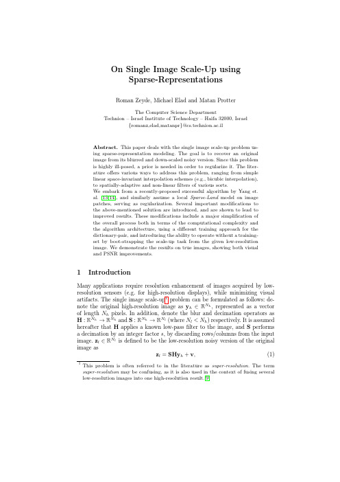
root mean square error (RMSE)
15
10
5
0
0
4
81216 Nhomakorabea20
24
28
32
shift in [pixels]
Fig. 1: Shift dependency of the multiresolution
fusion methods (see text for details)
The dotted line indicates the shift error when the Haar
timm中randomresizedcropandinterpolation解释

timm中randomresizedcropandinterpolation解释在timm(PyTorch Image Models)中,randomresizedcropandinterpolation是一个预处理函数,用于对图像进行随机裁剪和插值操作,旨在增加输入图像的变化和多样性。
1.随机裁剪:随机裁剪是一种常用的数据增强技术,通过从原始图像中随机采样一个区域,并将其缩放到固定大小作为网络的输入。
具体来说,从原始图像中随机采样一个矩形区域,该区域的大小在一定的范围内(例如,0.08~1之间)。
然后将采样区域缩放到固定大小(例如,224×224),作为网络的输入。
此外,随机水平翻转图像(以50%的概率)可以增加数据的随机性。
由于随机裁剪是随机进行的,因此可以增加数据的多样性和泛化能力,降低模型的过拟合风险。
2.插值:插值是一种将低分辨率的图像转换为高分辨率图像的技术,通过近似原始图像中缺失的像素值,重建出一幅更加清晰的图像。
插值的实现方式包括获取低分辨率图像,然后使用插值算法对图像进行重建。
常用的插值算法包括最近邻插值、双线性插值和双三次插值等。
其中,双线性插值是最常用的一种,它将缺失的像素值通过对周围四个最近邻像素值的加权平均计算得出。
在深度学习中,插值常常和随机裁剪结合使用,以提高图像的分辨率和清晰度。
总的来说,randomresizedcropandinterpolation的工作原理是首先对图像进行随机裁剪,然后将裁剪后的图像进行插值处理。
这种预处理方法能够增加模型训练时数据的变化和多样性,从而提升模型的泛化能力。
如需更多关于timm中randomresizedcropandinterpolation的解释信息,建议咨询计算机领域专业人士或查阅相关资料。
feed forward network表达公式

在深度学习领域中,feed forward network(前馈神经网络)是一种常见的神经网络结构,其表达公式包含了多个层次和复杂的数学运算。
在本文中,我将从简单到复杂、由浅入深地解释和探讨feed forward network表达公式,以帮助你全面理解这一主题。
让我们从最基本的层次开始,来理解feed forward network的表达公式。
一个简单的单层神经网络可以表示为:\[ z = \sum_{i=1}^{n} w_i * x_i + b \]其中,\( z \) 为神经元的输出,\( w_i \) 为输入 \( x_i \) 的权重,\( b \) 为偏置项。
这个表达式描述了神经元对输入信号的加权和,再加上偏置项的运算过程。
将这个结果带入激活函数中,比如Sigmoid函数或ReLU函数,就可以得到神经元的最终输出。
当我们将多个这样的神经元连接在一起,形成一个多层神经网络时,表达公式就会变得更加复杂。
假设我们有一个包含多个隐藏层的深度前馈网络,其表达公式可以表示为:\[ a^{(l)} = g(z^{(l)}) \]\[ z^{(l)} = W^{(l)} * a^{(l-1)} + b^{(l)} \]其中,\( a^{(l)} \) 为第 \( l \) 层的激活值,\( z^{(l)} \) 为加权输入值,\( W^{(l)} \) 为第 \( l \) 层的权重矩阵,\( b^{(l)} \) 为偏置向量,\( g(\cdot) \) 为激活函数。
这样,通过逐层计算每层的输出,就可以得到整个网络的输出。
在实际应用中,为了提高网络的性能,人们还会使用一些改进的技术,比如Batch Normalization、Dropout等,这些技术也会影响到前馈神经网络的表达公式和计算过程。
feed forward network表达公式涵盖了多层神经元的复杂计算过程,其公式包括了权重矩阵、偏置向量和激活函数等要素。
On Single Image Scale-Up using Sparse-Representations(Michael Elad 的文章)
2
Roman Zeyde, Michael Elad and Matan Protter
for an additive i.i.d. white Gaussian noise, denoted by v ∼ N 0, σ2I . Given zl, the problem is to find yˆ ∈ RNh such that yˆ ≈ yh. Due to the
hereafter that H applies a known low-pass filter to the image, and S performs
a decimation by an integer factor s, by discarding rows/columns from the input
{romanz,elad,matanpr}@cs.technion.ac.il
Abstract. This paper deals with the single image scale-up problem using sparse-representation modeling. The goal is to recover an original image from its blurred and down-scaled noisy version. Since this problem is highly ill-posed, a prior is needed in order to regularize it. The literature offers various ways to address this problem, ranging from simple linear space-invariant interpolation schemes (e.g., bicubic interpolation), to spatially-adaptive and non-linear filters of various sorts. We embark from a recently-proposed successful algorithm by Yang et. al. [13,14], and similarly assume a local Sparse-Land model on image patches, serving as regularization. Several important modifications to the above-mentioned solution are introduced, and are shown to lead to improved results. These modifications include a major simplification of the overall process both in terms of the computational complexity and the algorithm architecture, using a different training approach for the dictionary-pair, and introducing the ability to operate without a trainingset by boot-strapping the scale-up task from the given low-resolution image. We demonstrate the results on true images, showing both visual and PSNR improvements.
4.image_interpolation

Interpolate at 1/2-pixel
f(x)=[0,60,120,150,180,150,120,60,0], x=n/2
Interpolate at 1/3-pixel
f(x)=[0,20,40,60,80,100,120,130,140,150,160,170,180,…], x=n/6
10
Linear Interpolation Formula
Heuristic: the closer to a pixel, the higher weight is assigned Principle: line fitting to polynomial fitting (analytical formula) f(n) f(n+a) f(n+1)
x
b
Since |a-c|>|b-d| x=(b+d)/2=black
NEDI Step 1: Interpolate diagonal pixels*
Image Interpolation
• Introduction
• Interpolation Techniques
– What is image interpolation? (D-A conversion) – Why do we need it?
• Interpolation Applications
EE465: Introduction to Digital Image Processing
12
1D Third-order Interpolation (Cubic)*
f(n) n
f(x)
x Cubic spline fitting
Fruit Image Classification Using Deep Learning

Fruit Image Classification Using Deep LearningHarmandeep Singh Gill;Osamah Ibrahim Khalaf;Youseef Alotaibi;Saleh Alghamdi;Fawaz Alassery【期刊名称】《计算机、材料和连续体(英文)》【年(卷),期】2022()6【摘要】Fruit classification is found to be one of the rising fields in computer and machine vision.Many deep learning-based procedures worked out so far to classify images may have some ill-posed issues.The performance of the classification scheme depends on the range of captured images,the volume of features,types of characters,choice of features from extracted features,and type of classifiers used.This paper aims to propose a novel deep learning approach consisting of Convolution Neural Network(CNN),Recurrent Neural Network(RNN),and Long Short-TermMemory(LSTM)application to classify the fruit images.Classification accuracy depends on the extracted and selected optimal features.Deep learning applications CNN,RNN,and LSTM were collectively involved to classify the N is used to extract the image features.RNN is used to select the extracted optimal features and LSTM is used to classify the fruits based on extracted and selected images features by CNN andRNN.Empirical study shows the supremacy of proposed over existing Support Vector Machine(SVM),Feed-forwardNeural Network(FFNN),and Adaptive Neuro-Fuzzy Inference System(ANFIS)competitive techniques forfruit images classification.The accuracy rate of the proposed approach is quite better than the SVM,FFNN,and ANFIS schemes.It has been concluded that the proposed technique outperforms existing schemes.【总页数】16页(P5135-5150)【作者】Harmandeep Singh Gill;Osamah Ibrahim Khalaf;Youseef Alotaibi;Saleh Alghamdi;Fawaz Alassery【作者单位】Department of Computer Science Arjan Dev Khalsa College Chohla Sahib;Al-Nahrain University-Nahrain Nano-Renewable Energy Research Center;Department of Computer Science of Computer and Information Systems Al-Qura University Arabia;Department of Information Technology of Computers and Information Technology University Arabia;Department of Computer Engineering of Computers and Information Technology University Arabia【正文语种】中文【中图分类】TP1【相关文献】1.An automated deep learning based pancreatic tumor diagnosis and classification model using computed tomography images2.Deep Learning-Based Classification of Fruit Diseases:An Application for Precision Agriculture3.An Integrated Deep Learning Framework for Fruits Diseases Classification4.Plant Disease Diagnosis and Image Classification Using Deep Learning5.Ensemble of Handcrafted and Deep Learning Model for Histopathological Image Classification因版权原因,仅展示原文概要,查看原文内容请购买。
- 1、下载文档前请自行甄别文档内容的完整性,平台不提供额外的编辑、内容补充、找答案等附加服务。
- 2、"仅部分预览"的文档,不可在线预览部分如存在完整性等问题,可反馈申请退款(可完整预览的文档不适用该条件!)。
- 3、如文档侵犯您的权益,请联系客服反馈,我们会尽快为您处理(人工客服工作时间:9:00-18:30)。
IMAGE INTERPOLATIONUSING FEEDFORWARD NEURAL NETWORKHironori AOKAGE*, Keisuke KAMEYAMA**, and Koichi WADA**Department of Computer Science**Department of Risk EngineeringUniversity of TsukubaTsukuba, Ibaraki, JapanE-mail: aokage@padc.cs.tsukuba.ac.jp, kame@emerald.risk.tsukuba.ac.jp, wada@cs.tsukuba.ac.jpABSTRACTAs various kinds of output devices emerged, such as high-resolution printers or a display of PDA(Personal Digital Assistant), the importance of high-quality resolution conversion has been increasing. This paper proposes a new method for enlarging image with high quality. One of the largest problems on image enlargement is the exaggeration of the jaggy edges. To remedy this problem, we propose a new interpolation method, which uses artificial neural network to determine the optimal values of interpolated pixels. The experimental results are shown and evaluated. The effectiveness of our methods is discussed by comparing with the conventional methods. KEY WORDSdigital image, resolution conversion, high quality, artificial neural network, feedforward network1. IntroductionRetaining quality in converting image resolution is important since images are often displayed or printed by output devices with various resolutions. Generally, the resolution of an image is determined by considering the resolution of a specific output device to which the image is to be output, together with the size of storage devices and/or network bandwidth. Thus, it is not possible to prepare an image that has an optimal resolution for all printers, displays, or network environment.One of the largest issues in converting image resolution is appearing of jaggy edges, especially when digital images are enlarged. The jaggy is inevitable because digital images are sampled in 2D lattice. In order to improve the quality of enlarged image, this problem cannot be ignored since edges have great influence on entire image quality. The method based on an adaptively transformed sampling function can remedy the jaggy problem [6]. In this method, sampling function is transformed adaptively to the values of neighbouring pixels. The algorithm of this method divided into two steps: 1)edges in the image are extracted and detected their direction, 2)sampling function is then transformed along the direction of these detected edges. This method can produce high-quality results. However, the drawback is in the amount of computation required.This paper presents a new method of image interpolation using a feedforward neural network. Required computation of the proposed method is less enough to be applicable to moving pictures as well. Furthermore, neural network’s capability as an optimal function generator can improve the quality of resulting image compared to the image by an adaptively transformed sampling function.In this paper, we focus on enlargement of images, since enlargement is more critical than reduction in terms of quality. The rest of this paper is organized as follows: In section 2, we will give a brief explanation on conventional methods of resolution conversion and describe the methods proposed by our laboratory. Section 3 proposes an approach which enlarges images using artificial neural network. Experimentation and evaluation of the proposed method are described in Section 4 and 5. Section 6 concludes our discussions and present our future plans.2. Interpolation of image pixelsInterpolation is a process of generating pixels derived from sampled pixels. The quality of the interpolated image highly depends on the interpolation algorithm. In this section, we will give overview of the conventional methods and discuss issues in interpolation.2.1 Conventional methodsBicubic convolution [1][2][3] is a well-known interpolation method, which can enlarge image with high quality. A value of a generated pixel is determined using the values of sixteen original pixels surrounding it. Using approximated sinc function [4], convolution operations are performed along x and y axes, or vice versa, independently. Thus, interpolation must be applied twice. Also, the interpolation will include error generated in two interpolations. This irrationally degrades image quality.Fig.1 Two-dimensional sampling functionfunctionFig.3 Sampling function of starfish2.2 Two-dimensional sampling functionBased on the one-dimensional sampling function, the two-dimensional sampling function is configured upon distance from sampling point, and defined as follows:)(),(223][3][y x y x s s +=ψξ (1)Here, )(3][t s ψ is a one-dimensional sampling function which is used in bicubic convolution.This way, original sample points will equally affect the points that are equidistantly located from them. The form of sampling function is shown in Fig.1.In the literature [5], subjective evaluation has been done by comparing with the images converted by the conventional method.2.3 Adaptively transformed sampling functionIn the methods mentioned above, the important issue that must be considered is appearing of jaggy edges. Jaggy edges appear due to the use of a single uniform interpolation function. In the method of using adaptively transformed sampling function [6], interpolation is performed using a two-dimensional function whose shapeis transformed along the edge of the image. We call this transformed function as Starfish .In starfish, two-dimensional sampling function is transformed with eight parameters as shown in Fig.2. Three-dimensional view of the starfish is shown in Fig.3. The algorithm of this method is as follows:To determine the shape of the sampling function, the influence from the surrounding sampled pixels to the objective interpolated pixel is calculated. At first, reduction rates toward the surrounding eight pixels are calculated. The shape of the function to each direction is reduced when an edge exists between the objective pixel and its neighbouring pixel. Thus, the transformation ratio for each axis is determined from the values of eight neighbouring sampled pixels.In this process, the global edge shape is not yet considered. The edge direction determined is based only on its local information, and does not always match the global edge shape. The next step is to determine the globally adequate transformation. This is done by incorporating the transformation ratio of each neighbouring pixel to the objective pixel iteratively.In our laboratory, we implement this method and apply to actual image data. The result is compared with images reconstructed by two-dimensional sampling function. In adaptively transformed sampling function method, the jaggy edge is not conspicuous because an edge is enlarged smoothly compared with an image enlarged with two-dimensional sampling function.However, this method requires large amount of computation. In addition, the transformation of the sampling function with this method is not necessarily optimal.3. Enlargement with artificial neural networksIn this section, interpolation method using Artificial Neural Networks(ANN) [7] is presented. Proposed method requires less computation, which can be applied to moving pictures. Using high resolution image on network training, optimal image interpolation can be achieved as well in proposed method. ANN is introduced briefly in the subsection that follows, then, the implementation of the image enlargement system using ANN is described.3.1 Artificial neural networksANN is an artificial network, which imitate living body neuron, and has been guaranteed that any type of functions can be approximated with high accuracy. There exist many types and architectures of ANN, e.g. Perceptron, RBF, or self-organizing map. In this paper, we focus on multilayer feedforward network structures. The neuron is a fundamental unit to operate ANN. Fig.4 shows a mathematical model of a neuron with N inputs.Here,N x x x ,....,,21are the input signals;N w w w ,....,,21are the synaptic weights of neuron; S is the signal after summing up inputs and weights; and y isthe output signal of the neuron.Neurons can be described mathematically by the following set of equations:∑==Ni i i w x S 1(2))(θ−=S f y (3)Here, θdepicts threshold value, and f is some activationfunction. The activation function is generally nonlinear. In general, sigmoid function is used as shown below:zez sigmoid α−+=11)( (4) The objective of training such a neural network is to determine the synaptic weights to produce final outputs as close to the target values as possible for all training patterns.Fig.5 shows the model of feedforward network. In this paper, we use backpropagation algorithm [8], which is the most common algorithm for multilayer feedforward network training. In the figure, L x x x ,....,21depict the network inputs and P y y y ,....,,21depict the network outputs, respectively. The layers are indicated as I , H , and O . The number of l depicts the number between each layers and i means the number of neuron in each layer. In this algorithm, each time a training for a pattern is finished, synaptic weights are updated.3.2 ImplementationIn this section, we will describe the detail of the implementation.Fig.6 shows the flow chart of the image enlargement system using ANN. As shown in the figure, the system consists of five parts of processes indicated by rectangles, and data files indicated by dotted rectangles.The detail of each process in the figure will be described below.1) Generating training setIn the method using starfish function, the transformation ratios for the interpolated pixel are determined by the neighbouring 64(8x8) sampled points. Thus, in this section, it is assumed that the number of network input is 64(8x8) as a example. Fig. 7 shows the process of determining a training set from an original image when the image is enlarged doubly.The outline of generating the training set is as follows. The first figure(Fig. 7(a)) shows the original image for training and white circles depict the pixels. At first, 64 pixels indicated by gray circles are selected for network inputs(Fig. 7(b)). As the correct values, which is to be compared with output values, four pixels are selectedfrom original image(shown as black circles in the figure (c)). This set of 64 pixels and four pixels is a pattern of a training set. Then, as shown in the figure (d), the next training pattern is generated in the same way as described above. After generating all patterns of a training set, they are saved as a TS file.1x x x yFig.4 Artificial neuronx Py 1y x 2y 1x 1=l 2=l H OFig.5 Feedforward network2) Network trainingFor training, the gradient descent algorithm is used. The detail of the algorithm can be found in [9]. In this process, TS file, which is created in previous process is used as a training set. After training, network status with synaptic weights is saved as a WT file .3) Estimating and interpolationThe pixels to be interpolated in the enlarged image are estimated using trained network. In this process, the image is separated into Red, Green, and Blue planes, and estimated individually using the same trained network. Finally, RGB planes are integrated to form a 24-bit bitmap image and saved as an IMG file. As a result, the image is enlarged doubly.4. ExperimentIn this section, we will describe the detail of the experimentation using ANN. The image for training, network architecture, and the original images are shown.4.1 Image for trainingIn training ANN, we used a bicycle image as shown in Fig.8. The image is greyscale, and consists of 332x420 pixels.Fig.6 Process of enlargement system with ANNFig.7 Process of generating training set4.2 Network architectureThe architecture of the ANN consists of three layers, aninput layer, a hidden layer, and an output layer. To changethe area size that affects to interpolated points, the numberof neurons of an input layer is varied as 16(4x4), 36(6x6),and 64(8x8). For each case, one extra input is added forbias. The output layer consists of four neurons. The number of neurons in the hidden layer is varied as 40, 45,and 50.The activation function we used is sigmoid function inboth hidden layer and output layer.4.3 Original imageJIS(Japan Industrial Standard) full color images, shown in Fig.9 are used as the original images. We used two kinds of images; “whole bicycle” and “lobster”. The size of “whole bicycle” is 616x772 and “lobster” is 492x316,respectively. As described in the section 4.1, the trainingis performed using a part of the original image “wholebicycle” as shown in Fig. 8.Fig.8 Image for using learning(a)whole bicycle(b)lobster (a)whole bicycle (b)lobsterFig.9 Original images5. EvaluationIn this section, we will evaluate the network architecture and quality of the interpolated image.5.1 Network architectureIn the network evaluation, the image is enlarged doubly with various parameters to find the optimal network architecture for image interpolation.The original image is “whole bicycle” shown in Fig.9(a).1) Input layerThe image is enlarged doubly with 16, 36, and 64 neurons in input layer, with the 45-neurons hidden layer.The results of interpolation with each parameter are shown in Fig.10. The figures show a part of the resulting image. The results show that the noise is observed in the images interpolated with 16 neurons input and 64 neurons input, while the result with 36 neurons yields less noise compared with others. It has been confirmed that input of 36 neurons is optimal for image interpolation.2) Hidden layerIn this evaluation, the image is enlarged using the network with 40, 45, and 50 neurons in hidden layer. The number of input neurons is 36.The parts of result images are shown in Fig.11. Comparing with the image interpolated by the network with 40-neurons in hidden layer, jaggy edges are less conspicuous by the networks with 45-neurons. 50-neuronsnetwork produces a image with almost the same quality as the one with 45-neurons. Thus, 45-neurons hidden layer is appeared to be optimal.input=16input=36input=64Fig.10 Interpolation results with hidden=45hidden=40hidden=45hidden=50Fig.11 Interpolation result with input=365.2 Image qualityIn this evaluation, quality of the images enlarged bybicubic convolution, two-dimensional sampling function,starfish function, and the proposed method are compared.The results of interpolation are shown in Fig.12 andFig.13. The figures show a part of the resulting images.The results show that jaggy edges are observed in theimages interpolated by bicubic convolution and two-dimensional sampling function. Although the starfishproduces less jaggy images than the above conventionalmethods, smoothest edges are observed in the enlargedimages by the proposed method.It has been confirmed that the proposed method caninterpolate with higher quality than the conventionalmethod in the edge parts as well as the texture parts of theimage.6. ConclusionThis paper presents a new method of image interpolationusing an artificial neural network. The proposed methodrequires less computation than the conventional high-quality image interpolation methods. The algorithm of theproposed method was described in detail. To evaluate ourmethod, the proposed method is implemented and appliedto actual images. The optimal network architecture isdiscussed by comparing the quality of the imagesenlarged by various networks. The results show that ourmethod can produce high-quality enlarged images.As a future work, more extensive experiments usingvarious kinds of images are important to confirm theeffectiveness of our method.In addition, we are planning to design a hardware in orderto apply the proposed method to video images.References:[1]Andrew S.Glassner, ”Principles of Digital ImageSynthesis vol.1”, Morgan Kaufmann Publishers, 1995.[2]S.K.Park, “Image Reconstruction by ParametricCubic Convolution”, Computer Vision, Graphics, andImage Processing, Academic Press, Vol.23, pp258-272,1983.[3] D.P.Mitchel and A.N Netravali, “ReconstructionFilter in Computer Graphics”, ACM Computer Graphics.Vol.22, No.4, pp.221-228, 1988.[4] C.E.Shannon, “A mathematical theory ofcommunication”, Bell System Tech. J., vol. 27, pp. 379-423, 623-656, 1948.[5]H.Aokage, K.Wada, and K.Toraichi. “High QualityConversion of Image Resolution Using Two-DimensionalSampling Function”, Proc.of IEEE Pacific Rim Conf. onCommunication, Computers and Signal Processing, pp720-723, 2003.[6]M.Ohira, K.Mori, K.Wada and K.Toraichi, “HighQuality Image Restoration by adaptively TransformedSampling Function”, Proc. of IEEE Pacific Rim Conf. onCommunications, Computers and Signal Processing, pp.201-204, 1999.[7]S.Shekhar and M.B.Amin, “Generalization byNeural Networks”, IEEE Transactions on Knowledge andData Engineering, vol. 4, no. 2, pp. 177-185, April 1992.[8]Z.Y.Chen, M.Desai and X.P.Zhang, “FeedforwardNeural Networks with Multilevel Hidden Neurons forRemotely Sensed Image Classification”, Proc.of the 1997International Conference on Image Processing, pp. 653-655, 1997.[9] F.Diotalevi, M.Valle and D.D.Caviglia, “Evaluationof Gradient Descent Learning Algorithms With anAdaptive Local Rate Technique for HierarchicalFeedForward Architectures”, Proc. of the IEEE-INNS-ENNS International Joint Conference of Neural Networks,pp.2185-2190, 2000.(a)bicubic (b)two-dimensional sampling function(c)Starfish (d)ANNFig.12 lobster(a)bicubic (b)two-dimensional sampling function(c)Starfish (d)ANNFig.13 whole bicycle。