数学专业英语论文
数学与应用数学专业论文英文文献翻译

数学与应用数学专业论文英文文献翻译Chapter 3InterpolationInterpolation is the process of defining a function that takes on specified values at specified points. This chapter concentrates on two closely related interpolants, the piecewise cubic spline and the shape-preserving piecewise cubic named “pchip”.3.1 The Interpolating PolynomialWe all know that two points determine a straight line. More precisely, any two points in the plane, ),(11y x and ),(11y x , with )(21x x ≠ , determine a unique first degree polynomial in x whose graph passes through the two points. There are many different formulas for the polynomial, but they all lead to the same straight line graph.This generalizes to more than two points. Given n points in the plane, ),(k k y x ,n k ,,2,1 =, with distinct k x ’s, there is aunique polynomial in x of degree less than n whose graph passes through the points. It is easiest to remember that n , the number of data points, is also the number of coefficients, although some of the leading coefficients might be zero, so the degree might actually be less than 1-n . Again, there are many different formulas for the polynomial, but they all define the same function.This polynomial is called the interpolating polynomial because it exactly re- produces the given data.n k y x P k k ,,2,1,)( ==,Later, we examine other polynomials, of lower degree, that only approximate the data. They are not interpolating polynomials.The most compact representation of the interpolating polynomial is the La- grange form.∑∏⎪⎪⎭⎫ ⎝⎛--=≠k k k j j k j y x x x x x P )( There are n terms in the sum and 1-n terms in each product, so this expression defines a polynomial of degree at most 1-n . If )(x P is evaluated at k x x = , all the products except the k th are zero. Furthermore, the k th product is equal to one, so the sum is equal to k y and theinterpolation conditions are satisfied.For example, consider the following data set:x=0:3;y=[-5 -6 -1 16];The commanddisp([x;y])displays0 1 2 3-5 -6 -1 16 The Lagrangian form of the polynomial interpolating this data is)16()6()2)(1()1()2()3)(1()6()2()3)(2()5()6()3)(2)(1()(--+----+---+-----=x x x x x x x x x x x x x P We can see that each term is of degree three, so the entire sum has degree at most three. Because the leading term does not vanish, the degree is actually three. Moreover, if we plug in 2,1,0=x or 3, three of the terms vanish and the fourth produces the corresponding value from the data set.Polynomials are usually not represented in their Lagrangian form. More fre- quently, they are written as something like523--x xThe simple powers of x are called monomials and this form of a polynomial is said to be using the power form.The coefficients of an interpolating polynomial using its power form,n n n n c x c x c x c x P ++++=---12211)(can, in principle, be computed by solving a system of simultaneous linear equations⎥⎥⎥⎥⎦⎤⎢⎢⎢⎢⎣⎡=⎥⎥⎥⎥⎦⎤⎢⎢⎢⎢⎣⎡⎥⎥⎥⎥⎥⎦⎤⎢⎢⎢⎢⎢⎣⎡------n n n n n n n n n n n y y y c c c x x x x x x x x x 21212122212121111111 The matrix V of this linear system is known as a Vandermonde matrix. Its elements arej n kj k x v -=, The columns of a Vandermonde matrix are sometimes written in the opposite order, but polynomial coefficient vectors in Matlab always have the highest power first.The Matlab function vander generates Vandermonde matrices. For our ex- ample data set,V = vander(x)generatesV =0 0 0 11 1 1 18 4 2 127 9 3 1Thenc = V\y’computes the coefficientsc =1.00000.0000-2.0000-5.0000In fact, the example data was generated from the polynomial 523--x x .One of the exercises asks you to show that Vandermonde matrices are nonsin- gular if the points k x are distinct. But another one of theexercises asks you to show that a Vandermonde matrix can be very badly conditioned. Consequently, using the power form and the Vandermonde matrix is a satisfactory technique for problems involving a few well-spaced and well-scaled data points. But as a general-purpose approach, it is dangerous.In this chapter, we describe several Matlab functions that implement various interpolation algorithms. All of them have the calling sequencev = interp(x,y,u)The first two input arguments, x and y, are vectors of the same length that define the interpolating points. The third input argument, u, is a vector of points where the function is to be evaluated. The output, v, is the same length as u and has elements ))xterpyvuink(k(,,)(Our first such interpolation function, polyinterp, is based on the Lagrange form. The code uses Matlab array operations to evaluate the polynomial at all the components of u simultaneously.function v = polyinterp(x,y,u)n = length(x);v = zeros(size(u));for k = 1:nw = ones(size(u));for j = [1:k-1 k+1:n]w = (u-x(j))./(x(k)-x(j)).*w;endendv = v + w*y(k);To illustrate polyinterp, create a vector of densely spaced evaluation points.u = -.25:.01:3.25;Thenv = polyinterp(x,y,u);plot(x,y,’o’,u,v,’-’)creates figure 3.1.Figure 3.1. polyinterpThe polyinterp function also works correctly with symbolic variables. For example, createsymx = sym(’x’)Then evaluate and display the symbolic form of the interpolating polynomial withP = polyinterp(x,y,symx)pretty(P)produces-5 (-1/3 x + 1)(-1/2 x + 1)(-x + 1) - 6 (-1/2 x + 3/2)(-x + 2)x-1/2 (-x + 3)(x - 1)x + 16/3 (x - 2)(1/2 x - 1/2)xThis expression is a rearrangement of the Lagrange form of the interpolating poly- nomial. Simplifying the Lagrange form withP = simplify(P)changes P to the power formP =x^3-2*x-5Here is another example, with a data set that is used by the other methods in this chapter.x = 1:6;y = [16 18 21 17 15 12];disp([x; y])u = .75:.05:6.25;v = polyinterp(x,y,u);plot(x,y,’o’,u,v,’-’);produces1 2 3 4 5 616 18 21 17 15 12creates figure 3.2.Figure 3.2. Full degree polynomial interpolation Already in this example, with only six nicely spaced points, we canbegin to see the primary difficulty with full-degree polynomial interpolation. In between the data points, especially in the first and last subintervals, the function shows excessive variation. It overshoots the changes in the data values. As a result, full- degree polynomial interpolation is hardly ever used for data and curve fitting. Its primary application is in the derivation of other numerical methods.第三章 插值多项式插值就是定义一个在特定点取给定值得函数的过程。
数学论文英语写作范文
120词英语范文-帮忙:2篇英语作文(120字以上)高二水准,2篇英第一片 Is a Training Class or Family Teacher Necessary? More and more middle school students are going to all kinds of training classes or having family teachers at the weekend。
There are two different viewpoints about it。
On the one hand, some think that studying following the family teachers is better than self study。
In my opinion, as students, we should really know whether we need a training class or family teacher。
First, make sure that you need them, and they would be helpful, then choose a reasonable one。
Just remember, once you start and never give up。
关于数学的作文关于数学的作文 200字的篇一:关于数学生活中,处处有数学。
例如:买菜啦!买文具啦!量布等等,都需要用到数学。
这个学期,老师教了一个新知识,是小数的乘法和除法。
这个知识,可帮了我大忙啊!昨天晚上,我妈妈一起去买桔子。
桔子是1.8元一斤,妈妈买了4.5斤,本应该付钱8.1元。
可是营业员粗心大意,不知道怎么算的,算成了9元钱。
还好我利用了这个学期新教的知识,在脑子里算过一便后,马上纠正了营业员的失误。
不仅营业员阿姨夸我聪明,这么小都会小数乘除法了,而且在回家的路上,妈妈还表扬我,给她省了0.9元,并且学过的知识能在生活中活用。
数学专业英语论文
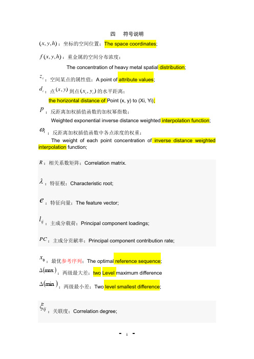
四 符号说明),,(h y x :坐标的空间位置;The space coordinates;),,(h y x f :重金属的空间分布浓度;The concentration of heavy metal spatial distribution;i z :空间某点的属性值;A point of attribute values;i d :点),(y x 到点),(i i y x 的水平距离;the horizontal distance of Point (x, y) to (Xi, Yi);p :反距离加权插值函数的加权幂指数;Weighted exponential inverse distance weighted interpolation function; i ω :反距离加权插值函数中各点浓度的权重; The weight of each point concentration of inverse distance weighted interpolation function; R :相关系数矩阵;Correlation matrix. λ:特征根;Characteristic root;e :特征向量;The feature vector;ij l :主成分载荷;Principal component loadings;PC :主成分贡献率;Principal component contribution rate;0x :最优参考序列;The optimal reference sequence;()max ∆:两级最大差;two Level maximum difference()min ∆:两级最小差;Two level smallest difference;ij ξ:关联度;Correlation degree;i E :综合评价系数;Comprehensive evaluation coefficient;:ε隶属度系数;Membership degree coefficient;ihC ': 第i 个评价因子污染强度最大的超标值(以p 级准则值为界); the largest pollution exceeding the standards value of the ith evaluation factor intensity (p grade criterion value for the sector);ip S :第i 个评价因子p 级准则限值;The ith evaluation factor intensity of P grade criterion limit;r :超标因子个数;The number of Exceed the standard factors;n :评价因子总数,当0=r 时,取0=ε;The total number of evaluation factor, when 0=r , 0=ε;i d :各区"i C 与"1S 之间的相对距离;The relative distance between the "i C and "1S ;j δ:各级标准隶属度向量"j S 与"1S 之间的相对距离。
数学专业英语 第六讲 论文写作 常见错误分析

不要过于烦琐.
• 不要用On the Study of ... 或On the Existence of... 之类作为 标题.
• 标题通常是一个名词性短语, 不是一个完整的句子,
• 无需主、谓、宾齐全, 其中的动词一般以分词或动名词的 形式出现, 有时冠词可以省略. • 偶尔有以疑问句为标题的论文, 但不应以陈述句为标题. • 为方便二次检索, 标题尽量避免使用复杂的数学式子.
• [2] name(s) of author(s), title of the book (in italics),
publishinghouse, city of publication, year of publication.
16
Mathematical English
• [3] name(s) of author(s), title of the paper, in: title of the book (in italics), publishing house, city of publication, year of publication, numbers of the first and last pages of the paper.
improvements for you.
9
Mathematical English
数学论文对英语的要求其实并不高. 而且我们有功能强大的 LATEX(WinEdt) 编辑软件, 可以轻而易举地编排出有复
杂公式、美观漂亮的版面.
但是, 有些作者在论文写作中存在不少问题.
下面从论文的各个组成部分对一些常见的错误进行分析并举
发表论文的目的, 一是公开自己的成果并得到学术界的承认, 二是为了同行之间的交流.
数学专业英语2-11C(精选5篇)
数学专业英语2-11C(精选5篇)第一篇:数学专业英语2-11C数学专业英语论文数学专业英语论文英文原文:2-12CSome basic principles of combinatorial analysisMany problems in probability theory and in other branches of mathematics can be reduced to problems on counting the number of elements in a finite set. Systematic methods for studying such problems form part of a mathematical discipline known ascombinatorial analysis. In this section we digress briefly to discuss some basic ideas in combinatorial analysis that are useful in analyzing some of the more complicated problems of probability theory.If all the elements of a finite set are displayed before us, there is usually no difficulty in counting their total number. More often than not, however, a set is described in a way that makes it impossible or undesirable to display all its elements. For example,we might ask for the total number of distinct bridge hands that can be dealt. Each player is dealt 13 cards from a 52-card deck. The number of possible distinct hands is the same as the number of different subsets of 13 elements that can be formed from a set of 52 elements.Since this number exceeds 635 billion, a direct enumeration of all the possibilities is clearly not the best way to attack this problem; however, it can readily be solved by combinatorial analysis.This problem is a special case of the more general problem of counting the number of distinct subsets of k elements that may be formed from a set of n elements (When we say that a set has n elements,we mean that it has n distinct elements.Such a set is sometimes called an n-element set.),where n k. Let us denote this number by f(n,k).It has long been known thatn(12.1)f(n,k)k,n where, as usual k denotes the binomial coefficient,n n!k k!(n k)!52In the problem of bridge hands we havef(52,13)13635,013,559,600different hands that a player can be dealt.There are many methods known for proving (12.1). A straightforward approach is to form each subset of k elements by choosing the elements one at a time. There are n possibilities for the first choice, n 1 possibilities for the second choice, and n(k1) possibilities for the kth choice. If we make all possible choices in this1manner we obtain a total ofn(n1)(n k1)n! (n k)!subsets of k elements. Of course, these subsets are not all distinct. For example, ifk3the six subsetsa,b,c,b,c,a,c,a,b,a,c,b,c,b,a, b,a,carc all equal. In general, this method of enumeration counts each k-element subset exactly k! times. Therefore we must divide the number n!/(n k)! by k! to n obtain f(n,k). This gives us f(n,k)k, as asserted.译文:组合分析的一些基本原则许多概率论和其他一些数学分支上的问题,都可以简化成基于计算有限集合中元素数量的问题。
数学专业英语作文(学习体会)[五篇材料]
![数学专业英语作文(学习体会)[五篇材料]](https://img.taocdn.com/s3/m/383bbffba0c7aa00b52acfc789eb172ded639928.png)
数学专业英语作文(学习体会)[五篇材料]第一篇:数学专业英语作文(学习体会)About learning the Mathematics English We major in Information and computing science , which belongs to Department of Mathematics.And also we need to learn Mathematics English in this term.As a smoothly through this term student , I benefited a lot.Firstly , I think learning English needs a lot of practice.We need to practice listening , writing , reading and thinking in English.But for the Math ematics English , it’s difficult.Because there are many different.Mathematics English always describe objective facts and truth.There are many long sentence and professional words and phrases , which is different to our Oral English.So learning Mathematics English is a challenge.Unfortunately , I don’t learn it well.Although English is the common language of communications for world diplomacy, economics and defence, then let us be as fluent and proficient in it as possible, for the sake of our own country's advancement and prestige.May be we will repent learning poorly in Mathematics English when we write graduation thesis for searching the English thesis.Secondly , I learn a little about Mathematics English.We study some texts about Mathematics, Equation ,Geometry ,Set , Function , Sequences and Their Limits , The Derivative of a Function , Elementary Mathematical Logic and so on.Also I learn some useful things , for example , some professional words and phrases , and how to describe some sample objective facts and truth , how to describe some sample formula in English.May be it helpless in my graduation thesis , but it will keeps in my mind for many years!Thirdly , the teacher’s teaching methods is very well.Hegave us a stage and let us play fully!We can learn together and there full of cordial and friendly atmosphere where we can make common progress and common development.Some students seized the opportunity but some let the chance slip away.I caught the opportunity and did my best!Thank for teacher giving the stage let me play my role!To sum up, my college life and learning life still exist many shortcomings.I will be in the next few months of this struggle, make oneself to make greater progress.第二篇:专业英语学习体会专业英语学习体会英语作为一门重要的学科,正在由于科技的飞速发展、信息全球化、社会化的日趋接近以及国际语言的特殊身份而身价倍增,成为了跨入二十一世纪所必备的三张通行证之一。
数学专业英语(Doc版).14

数学专业英语-MathematicansLeonhard Euler was born on April 15,1707,in Basel, Switzerland, the son of a mathematician and Caivinist pastor who wanted his son to become a pastor a s well. Although Euler had different ideas, he entered the University of Basel to study Hebrew and theology, thus obeying his father. His hard work at the u niversity and remarkable ability brought him to the attention of the well-known mathematician Johann Bernoulli (1667—1748). Bernoulli, realizing Euler’s tal ents, persuaded Euler’s father to change his mind, and Euler pursued his studi es in mathematics.At the age of nineteen, Euler’s first original work appeared. His paper failed to win the Paris Academy Prize in 1727; however this loss was compensated f or later as he won the prize twelve times.At the age of 28, Euler competed for the Pairs prize for a problem in astrono my which several leading mathematicians had thought would take several mont hs to solve.To their great surprise, he solved it in three days! Unfortunately, th e considerable strain that he underwent in his relentless effort caused an illness that resulted in the loss of the sight of his right eye.At the age of 62, Euler lost the sight of his left eye and thus became totally blind. However this did not end his interest and work in mathematics; instead, his mathematical productivity increased considerably.On September 18, 1783, while playing with his grandson and drinking tea, Eul er suffered a fatal stroke.Euler was the most prolific mathematician the world has ever seen. He made s ignificant contributions to every branch of mathematics. He had phenomenal m emory: He could remember every important formula of his time. A genius, he could work anywhere and under any condition.George cantor (March 3, 1845—June 1,1918),the founder of set theory, was bo rn in St. Petersburg into a Jewish merchant family that settled in Germany in 1856.He studied mathematics, physics and philosophy in Zurich and at the University of Berlin. After receiving his degree in 1867 in Berlin, he became a lecturer at the university of Halle from 1879 to 1905. In 1884,under the stra in of opposition to his ideas and his efforts to prove the continuum hypothesis, he suffered the first of many attacks of depression which continued to hospita lize him from time to time until his death.The thesis he wrote for his degree concerned the theory of numbers; however, he arrived at set theory from his research concerning the uniqueness of trigon ometric series. In 1874, he introduced for the first time the concept of cardinalnumbers, with which he proved that there were “more”transcendental numb ers than algebraic numbers. This result caused a sensation in the mathematical world and became the subject of a great deal of controversy. Cantor was troub led by the opposition of L. Kronecker, but he was supported by J.W.R. Dedek ind and G. Mittagleffer. In his note on the history of the theory of probability, he recalled the period in which the theory was not generally accepted and cri ed out “the essence of mathematics lies in its freedom!”In addition to his work on the concept of cardinal numbers, he laid the basis for the concepts of order types, transfinite ordinals, and the theory of real numbers by means of fundamental sequences. He also studied general point sets in Euclidean space a nd defined the concepts of accumulation point, closed set and open set. He wa s a pioneer in dimension theory, which led to the development of topology.Kantorovich was born on January 19, 1912, in St. Petersburg, now called Leni ngrad. He graduated from the University of Leningrad in 1930 and became a f ull professor at the early age of 22.At the age of 27, his pioneering contributi ons in linear programming appeared in a paper entitled Mathematical Methods for the Organization and planning of production. In 1949, he was awarded a S talin Prize for his contributions in a branch of mathematics called functional a nalysis and in 1958, he became a member of the Russian Academy of Science s. Interestingly enough, in 1965,kantorovich won a Lenin Prize fo r the same o utstanding work in linear programming for which he was awarded the Nobel P rize. Since 1971, he has been the director of the Institute of Economics of Ma nagement in Moscow.Paul R. Halmos is a distinguished professor of Mathematics at Indiana Univers ity, and Editor-Elect of the American Mathematical Monthly. He received his P h.D. from the University of Illinois, and has held positions at Illinois, Syracuse, Chicago, Michigan, Hawaii, and Santa Barbara. He has published numerous b ooks and nearly 100 articles, and has been the editor of many journals and se veral book series. The Mathematical Association of America has given him the Chauvenet Prize and (twice) the Lester Ford award for mathematical expositio n. His main mathematical interests are in measure and ergodic theory, algebraic, and operators on Hilbert space.Vito Volterra, born in the year 1860 in Ancona, showed in his boyhood his e xceptional gifts for mathematical and physical thinking. At the age of thirteen, after reading Verne’s novel on the voyage from earth to moon, he devised hi s own method to compute the trajectory under the gravitational field of the ear th and the moon; the method was worth later development into a general proc edure for solving differential equations. He became a pupil of Dini at the Scu ola Normale Superiore in Pisa and published many important papers while still a student. He received his degree in Physics at the age of 22 and was made full professor of Rational Mechanics at the same University only one year lat er, as a successor of Betti.Volterra had many interests outside pure mathematics, ranging from history to poetry, to music. When he was called to join in 1900 the University of Rome from Turin, he was invited to give the opening speech of the academic year. Volterra was President of the Accademia dei Lincei in the years 1923-1926. H e was also the founder of the Italian Society for the Advancement of Science and of the National Council of Research. For many years he was one of the most productive scientists and a very influential personality in public life. Whe n Fascism took power in Italy, Volterra did not accept any compromise and pr eferred to leave his public and academic activities.Vocabularypastor 牧师 hospitalize 住进医院theology 神学 thesis 论文strain 紧张、疲惫transcendental number 超越数relentless 无情的sensation 感觉,引起兴趣的事prolific 多产的controversy 争论,辩论depression 抑郁;萧条,不景气essence 本质,要素transfinite 超限的Note0. 本课文由几篇介绍数学家生平的短文组成,属传记式体裁。
数学建模论文英文
数学建模论文英文Abstract:Mathematical modeling is an essential tool in various scientific and engineering disciplines, facilitating the understanding and prediction of complex systems. This paper explores the fundamental principles of mathematical modeling, its applications, and the methodologies employed in constructing and analyzing models. Through case studies, we demonstrate the power of mathematical models in solving real-world problems.Introduction:The introduction of mathematical modeling serves as a foundation for the entire paper. It provides an overview of the significance of mathematical modeling in modern problem-solving and sets the stage for the subsequent sections. It also outlines the objectives and scope of the paper.Literature Review:This section reviews existing literature on mathematical modeling, highlighting the evolution of the field, key concepts, and the diverse range of applications. It also identifies gaps in current knowledge that the present study aims to address.Methodology:The methodology section describes the approach taken to construct and analyze mathematical models. It includes theselection of appropriate mathematical tools, the formulation of the model, and the validation process. This section is crucial for ensuring the scientific rigor of the study.Model Development:In this section, we delve into the process of model development, including the identification of variables, the establishment of relationships, and the formulation of equations. The development of the model is presented in a step-by-step manner to ensure clarity and reproducibility.Case Studies:Case studies are presented to demonstrate the practical application of mathematical models. Each case study is carefully selected to illustrate the versatility and effectiveness of mathematical modeling in addressing specific problems.Results and Discussion:This section presents the results obtained from the application of the mathematical models to the case studies. The results are analyzed to draw insights and conclusions about the effectiveness of the models. The discussion also includes an evaluation of the model's limitations and potential areas for improvement.Conclusion:The conclusion summarizes the key findings of the paper and reflects on the implications of the study. It also suggests directions for future research in the field of mathematical modeling.References:A comprehensive list of references is provided to acknowledge the sources of information and ideas presented in the paper. The references are formatted according to a recognizedcitation style.Appendices:The appendices contain any additional information that supports the paper, such as detailed mathematical derivations, supplementary data, or extended tables and figures.Acknowledgments:The acknowledgments section, if present, expresses gratitudeto individuals or organizations that contributed to the research but are not authors of the paper.This structure ensures that the mathematical modeling paperis comprehensive, logically organized, and adheres to academic standards.。
- 1、下载文档前请自行甄别文档内容的完整性,平台不提供额外的编辑、内容补充、找答案等附加服务。
- 2、"仅部分预览"的文档,不可在线预览部分如存在完整性等问题,可反馈申请退款(可完整预览的文档不适用该条件!)。
- 3、如文档侵犯您的权益,请联系客服反馈,我们会尽快为您处理(人工客服工作时间:9:00-18:30)。
课文9-B Terminology and notationwhen we work with a differential equation such as(9.1),it is customary to write y in place of f(x) and y' in place of f'(x),the higher derivatives being denoted by y",y''',etc.Of course ,other letters such as u,v,z,etc.are also used instead of y. By the order of an equation is meant the order of the highest derivatives which appears.For example ,(9.1)is first-order equation which may be written as y'=y.The differential equation)sin(xy"yxy'3+=is one of second order.In this chapter we shall begin our study with firs-order equations which can be solved for y' and written as follows:(9.2) y'=f(x,y),Where the expression f(x,y) on the right has various special forms. A defferentiable function y=Y(x) will be called a solution of (9.2) on an interval I if the function Y and and its derivative Y' satisfy the relationY'=f[x,Y(x)]For every x in I. The simplest case occurs when f(x,y)is independent of y.In this case , (9.2) becomes(9.3) y'=Q(x),Say, where Q is assumed to be a liven function defined on some interval I. To solve the differential equation(9. 3) means to find a primitive of Q.The Second fundamental theorem of calculus tells us how to do it when Q is continuous on an open interval I. We simply integrate Q and add any constant.Thus,every solution of (9.3) is included in the formula(9.4)y=∫Q(x)dx + C,where C is any constant ( usually called an arbitrary constant of integration). The differential equation(9.3) has infinitely many 课文9—B 术语和符号当我们在求解像(9.1)式的微分方程时,习惯用y代替f(x),用y’代替f'(x),用高阶导数y''和y'''等表示。
当然,其他的字母如u,v,z等等,同样可以用来代替y。
微分方程和阶数指的是现在其中的高阶导数的阶。
例如,(9.1)式是一个一次方程可以写成y'=y。
微分方程)s i n(x y"yxy'3+=是一个二阶的。
在这章我们将会学习到可以求解y'的一阶微分方程。
一阶方程可以被写成这样:(9.2)y'=f(x,y),其中,右边有各个特殊形式表示。
如果对于区间I中的每一个x函数y和他的倒数满足Y'=f[x,Y(x)]那么可微函数就为(9.2)在区间I中的一个解,最简单的形式是f(x,y)与y无关。
在这种情况下,(9.2)式变成了(9.3)y'=Q(x),表明,其中Q是假定在区间中的一个给定函数,对于一个给定的函数定义在各个区间I.求解微分方程(9.3)就意味着找到原始的区间Q。
第二基本积分定理告诉我们,当Q位于一个连续的开放的区间I 时该怎么做。
我们直接对Q积分并加上任意常数。
因此,y=∫Q(x)dx + C包含了(9.3)式的所有解(9.4)y=∫Q(x)dx + C,其中C为任意常数(通常被称为积分下限的任意常数),微分方程(9.3)有无穷多个解,每个解对应一个C。
solutions, one for each value of C.If it is not possible to evaluate the integral in(9. 4)in terms of familiar function,such as polynomials,rational functions,trigonometric and inverse trigonometric functions,logarithms,and exponentials,still we consider the differential equation as having been solved if the solution can be expressed in terms of integrals of known functions. In actual practice,there are various methods for obtaining approximate evaluations of integrals which lead to useful information about the solution. Automatic high-speed computing machines are often designed with this kind of problem in mind .Example. Linear motion determined from the velocity. Suppose a particle moves along a straight line in such a way that its velocity at time t is 2sin t.Determine its position at time t..Solution. if Y(t) denotes the position at time t measured from some staring point,then the derivative Y'(t) represents the velocity at time t. We are given thatY'(t)=2sin t. Integrating,we find thatY(t)=2∫sin t dt+C=2cos t +C.This is all we can deduce about Y(t) from a knowledge of the velocity alone;some other piece of information is needed to fix the position function. We can determine C if we know the value of Y at some particular instant. For example,if Y( 0)=0,then C=2 and the position function is Y( t )=2-2cos t. But if Y( 0)=2,then C=4 and the position function is Y( t)=4-2cos t.In some respects the example just solved is typical of what happens in general.Some-where in the process of solving a first-order differential equation,an integration is required to remove the derivative y' and in this step an arbitrary如果这不是在一些常见条件下的函数对(9.4)求积分,如多项式,有理方程,三角函数和反三角函数,对数和指数函数,我们仍然要把微分方程看作是一个被解答的函数,如果这个函数可以表示成已知的函数的话。
在实际的练习中,有很多方法可以获得近似值,这些值可以给正确答案提供很多有用的信息。
自动高速运行的计算机在设计时就常常考虑到对这类问题的处理。
例如:直线运动取决于速度。
假设一个质点按照这种方法沿着一条直线运动,它的速度在t时刻是 2sin t。
在t时刻确定该质点位置。
结论:如果Y(t)表示被测点在t时刻的位置,那么,Y'(t)表示在t时刻的速率。
我们便可得出以下结论:Y'(t)=2sin t.综上所述:Y(t)=2∫sin t dt+C=2cos t +C.这就是所有我们能从速度推断出的关于Y(t)的知识;其他的一些信息需要从位置函数中整理得到。
在一些特殊的时刻,如果我们知道Y值,便可推断出C。
例如,如果Y(0)=2,那么C=4,并且位置函数是:Y( t)=4-2cos t.在某些方面,刚才例题所解决的问题是一般情况下都可行。
在求解一阶微分方程的过程中,为了消除导数y',需要进一步进行积分,这时候就出现了一个任意常数C。
将常数Cconstant C appears. The way in which the arbitrary constant C enters into the solution will depend on the nature of the given differential equation. It may appear as an additive constant as in Equation(9. 4),but it is more likely to appear in some other way .For example,when we solve the equation y'=y in Section 9. 3,we shall find that every solution has the form y=Ce^x.In many problems it is necessary to select from the collection of all solutions one having a prescribed value at some point. The prescribed value is called an initial condition,and the problem of determining such a solution is called an initial-value problem.This terminology originated in mechanics where,as in the above example,the prescribed value represents the displacement at some initial time.熊进学号:20083729 代入方程的解决方法依赖于所给常微分方程。