数学专业英语论文(含中文版)
数学专业英语(Doc版).13
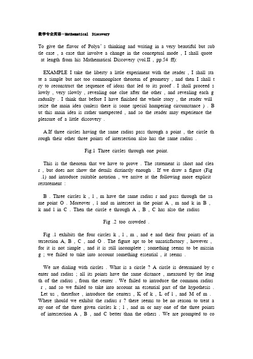
数学专业英语-Mathematical DiscoveryTo give the flavor of Polya’s thinking and writing in a very beautiful but sub tle case , a case that involve a change in the conceptual mode , I shall quote at length from his Mathematical Discovery (vol.II , pp.54 ff):EXAMPLE I take the liberty a little experiment with the reader , I shall sta te a simple but not too commonplace theorem of geometry , and then I shall t ry to reconstruct the sequence of idoas that led to its proof . I shall proceed s lowly , very slowly , revealing one clue after the other , and revealing each g radually . I think that before I have finished the whole story , the reader will seize the main idea (unless there is some special hampering circumstance ) . B ut this main idea is rather unexpected , and so the reader may experience the pleasure of a little discovery .A.If three circles having the same radius pass through a point , the circle th rough their other three points of intersection also has the same radius .Fig.1 Three circles through one point.This is the theorem that we have to prove . The statement is short and clea r , but does not show the details distinctly enough . If we draw a figure (Fig .1) and introduce suitable notation , we arrive at the following more explicit restatement :B . Three circles k , l , m have the same radius r and pass through the sa me point O . Moreover , l and m intersect in the point A , m and k in B , k and l inC . Then the circle e through A , B , C has also the radiusFig .2 too crowded .Fig .1 exhibits the four circles k , l , m , and e and their four points of in tersection A, B , C , and O . The figure apt to be unsatisfactory , however , for it is not simple , and it is still incomplete ; something seems to be missin g ; we failed to take into account something essential , it seems .We are dialing with circles . What is a circle ? A circle is determined by c enter and radius ; all its points have the same distance , measured by the leng th of the radius , from the center . We failed to introduce the common radius r , and so we failed to take into account an essential part of the hypothesis . Let us , therefore , introduce the centers , K of k , L of l , and M of m . Where should we exhibit the radius r ? there seems to be no reason to treat a ny one of the three given circles k ; l , and m or any one of the three points of intersection A , B , and C better than the others . We are prompted to connect all three centers with all the points of intersection of the respective circl e ; K with B , C , and O , and so forth .The resulting figure (Fig . 2) is disconcertingly crowded . There are so many lines , straight and circular , that we have much trouble old-fashioned maga zines . The drawing is ambiguous on purpose ; it presents a certain figure if you look t it in the usual way , but if you turn it to a certain position and lo ok at it in a certain peculiar way , suddenly another figure flashes on you , s uggesting some more or less witty comment on the first . Can you recognize i n our puzzling figure , overladen with straight and circles , a second figure th at makes sense ?We may hit in a flash on the right figure hidden in our overladen drawing , or we may recognize it gradually . We may be led to it by the effort to sol ve the proposed problem , or by some secondary , unessential circumstance . For instance , when we are about to redraw our unsatisfactory figure , we ma y observe that the whole figure is determined by its rectilinear part (Fig . 3) .This observation seems to be significant . It certainly simplifies the geometri c picture , and it possibly improves the logical situation . It leads us to restate our theorem in the following form .C . If the nine segmentsKO , KC , KB ,LC , LO , LA ,MB , MA , MO ,are all equal to r , there exists a point E such that the three segmentsEA , EB , EC ,are also equal to r .Fig . 3 It reminds you -of what ?This statement directs our attention to Fig . 3 . This figure is attractive ; it reminds us of something familiar . (Of what ?)Of course , certain quadrilaterals in Fig .3 . such as OLAM have , by hypo thesis , four equal sided , they are rhombi , A rhombus I a familiar object ; having recognized it , we can “see “the figure better . (Of what does the whole figure remind us ?)Oppositc sides of a rhombus are parallel . Insisting on this remark , we reali ze that the 9 segments of Fig . 3 . are of three kinds ; segments of the same kind , such as AL , MO , and BK , are parallel to each other . (Of what d oes the figure remind us now ?)We should not forget the conclusion that we are required to attain . Let us a ssume that the conclusion is true . Introducing into the figure the center E or the circle e , and its three radii ending in A , B , and C , we obtain (suppos edly ) still more rhombi , still more parallel segments ; see Fig . 4 . (Of wha t does the whole figure remind us now ?)Of course , Fig . 4 . is the projection of the 12 edges of a parallele piped h aving the particularity that the projection of all edges are of equal length .Fig . 4 of course !Fig . 3 . is the projection of a “nontransparent “parallelepiped ; we see o nly 3 faces , 7 vertices , and 9 edges ; 3 faces , 1 vertex , and 3 edges are invisible in this figure . Fig . 3 is just a part of Fig . 4 . but this part define s the whole figure . If the parallelepiped and the direction of projection are so chosen that the projections of the 9 edges represented in Fig . 3 are all equa l to r (as they should be , by hypothesis ) , the projections of the 3 remainin g edges must be equal to r . These 3 lines of length r are issued from the pr ojection of the 8th, the invisible vertex , and this projection E is the center o f a circle passing through the points A , B , and C , the radius of which is r .Our theorem is proved , and proved by a surprising , artistic conception of a plane figure as the projection of a solid . (The proof uses notions of solid g eometry . I hope that this is not a treat wrong , but if so it is easily redresse d . Now that we can characterize the situation of the center E so simply , it i s easy to examine the lengths EA , EB , and EC independently of any solid geometry . Yet we shall not insist on this point here .)This is very beautiful , but one wonders . Is this the “light that breaks fo rth like the morning . “the flash in which desire is fulfilled ? Or is it merel y the wisdom of the Monday morning quarterback ? Do these ideas work out in the classroom ? Followups of attempts to reduce Polya’s program to practi cal pedagogics are difficult to interpret . There is more to teaching , apparentl y , than a good idea from a master .——From Mathematical ExperienceVocabularysubtle 巧妙的,精细的clue 线索,端倪hamper 束缚,妨碍disconcert 使混乱,使狼狈ambiguous 含糊的,双关的witty 多智的,有启发的rhombi 菱形(复数)rhombus 菱形parallelepiped 平行六面体projection 射影solid geometry 立体几何pedagogics 教育学,教授法commonplace 老生常谈;平凡的。
数学专业英语(Doc版).Word4
数学专业英语-Continuous Functions of One Real VariableThis lesson deals with the concept of continuity, one of the most important an d also one of the most fascinating ideas in all of mathematics. Before we give a preeise technical definition of continuity, we shall briefly discuss the concep t in an informal and intuitive way to give the reader a feeling for its meanin g.Roughly speaking the situation is this: Suppose a function f has the value f ( p )at a certain point p. Then f is said to be continuous at p if at every ne arby point x the function value f ( x )is close to f ( p ). Another way of pu tting it is as follows: If we let x move toward p, we want the corresponding f unction value f ( x )to become arbitrarily close to f ( p ), regardless of the manner in which x approaches p. We do not want sudden jumps in the values of a continuous function.Consider the graph of the function f defined by the equation f ( x ) = x –[ x ], where [ x ] denotes the greatest integer < x. At each integer we have what is known ad a jump discontinuity. For example, f ( 2 ) = 0 ,but as x a pproaches 2 from the left, f ( x )approaches the value 1, which is not equal to f ( 2 ).Therefore we have a discontinuity at 2. Note that f ( x )does appro ach f ( 2 )if we let x approach 2 from the right, but this by itself is not en ough to establish continuity at 2. In case like this, the function is called conti nuous from the right at 2 and discontinuous from the left at 2. Continuity at a point requires both continuity from the left and from the right.In the early development of calculus almost all functions that were dealt with were continuous and there was no real need at that time for a penetrating loo k into the exact meaning of continuity. It was not until late in the 18th centur y that discontinuous functions began appearing in connection with various kind s of physical problems. In particular, the work of J.B.J. Fourier(1758-1830) on the theory of heat forced mathematicians the early 19th century to examine m ore carefully the exact meaning of the word “continuity”.A satisfactory mathematical definition of continuity, expressed entirely in term s of properties of the real number system, was first formulated in 1821 by the French mathematician, Augustin-Louis Cauchy (1789-1857). His definition, whi ch is still used today, is most easily explained in terms of the limit concept to which we turn now.The definition of the limit of a function.Let f be a function defined in some open interval containing a point p, altho ugh we do not insist that f be defined at the point p itself. Let A be a real n umber.The equationf ( x ) = Ais read “The limit of f ( x ), as x approached p, is equal to A”, or “f ( x )approached A as x approached p.”It is also written without the limit symb ol, as follows:f ( x )→A as x →pThis symbolism is intended to convey the idea that we can make f ( x )as close to A as we please, provided we choose x sufficiently close to p.Our first task is to explain the meaning of these symbols entirely in terms of real numbers. We shall do this in two stages. First we introduce the concept of a neighborhood of a point, the we define limits in terms of neighborhoods.Definition of neighborhood of a point.Any open interval containing a point p as its midpoint is called a neighborho od of p.NOTATION. We denote neighborhoods by N ( p ), N1( p ), N2( p )etc. S ince a neighborhood N( p )is an open interval symmetric about p, it consists of all real x satisfying p-r < x < p+r for some r > 0. The positive number r is called the radius of the neighborhood. We designate N ( p )by N ( p; r )if we wish to specify its radius. The inequalities p-r < x < p+r are equiv alent to –r<x-p<r,and to ∣x-p∣< r. Thus N ( p; r )consists of all points x whose distance from p is less than r.In the next definition, we assume that A is a real number and that f is a fun ction defined on some neighborhood of a point p(except possibly at p) . Th e function may also be defined at p but this is irrelevant in the definition.Definition of limit of a function.The symbolismf ( x ) = A or [ f ( x )→A as x→p ]means that for every neighborhood N1( A )there is some neighborhood N2( p)such thatf ( x )∈N1( A ) whenever x ∈N2( p ) and x ≠p (*)The first thing to note about this definition is that it involves two neighborho ods,N1( A) andN2( p). The neighborhood N1( A)is specified first; it tells us how close we wish f ( x )to be to the limit A. The second neighborhood, N2( p ),tells u s how close x should be to p so that f ( x ) will be within the first neighbor hood N1( A). The essential part of the definition is that, for every N1( A),n o matter how small, there is some neighborhood N2(p)to satisfy (*). In gener al, the neighborhood N2( p)will depend on the choice of N1( A). A neighbo rhood N2( p )that works for one particular N1( A) will also work, of course, for every larger N1( A), but it may not be suitable for any smaller N1( A).The definition of limit can also be formulated in terms of the radii of the n eighborhoodsN1( A)and N2( p ). It is customary to denote the radius of N1( A) byεan d the radius of N2( p)by δ.The statement f ( x )∈N1( A ) is equivalent to the inequality ∣f ( x ) –A∣<ε,and the statement x ∈N1( A) ,x ≠p ,is equivalent to the inequalities 0<∣x-p∣<δ. Therefore, the definition of limit can also be expressed as follows:The symbol f ( x ) = A means that for everyε> 0, there is aδ> 0 such th at∣f ( x ) –A∣<εwhenever 0 <∣x –p∣<δ“One-sided”limits may be defined in a similar way. For example, if f ( x )→A as x→p through values greater than p, we say that A is right-hand limi t of f at p, and we indicate this by writingf ( x ) = AIn neighborhood terminology this means that for every neighborhood N1( A) ,t here is some neighborhood N2( p) such thatf ( x )∈N1( A) wheneve r x ∈N1( A) and x > pLeft-hand limits, denoted by writing x→p-, are similarly defined by restricti ng x to values less than p.If f has a limit A at p, then it also has a right-hand limit and a left-hand li mit at p, both of these being equal to A. But a function can have a right-hand limit at p different from the left-hand limit.The definition of continuity of a function.In the definition of limit we made no assertion about the behaviour of f at the point p itself. Moreover, even if f is defined at p, its value there need not b e equal to the limit A. However, if it happens that f is defined at p and if it also happens that f ( p ) = A, then we say the function f is continuous at p. In other words, we have the following definition.Definition of continuity of a function at a point.A function f is said to be continuous at a point p if( a ) f is defined at p, and ( b ) f ( x ) = f ( p )This definition can also be formulated in term of neighborhoods. A function f is continuous at p if for every neighborhood N1( f(p))there is a neighborhood N2(p)such thatf ( x ) ∈N1( f (p)) whenever x ∈N2( p).In theε-δterminology , where we specify the radii of the neighborhoods, the definition of continuity can be restated ad follows:Function f is continuous at p if for every ε> 0 ,there is aδ> 0 such that ∣f( x ) –f ( p )∣< εwhenever ∣x –p∣< δIn the rest of this lesson we shall list certain special properties of continuou s functions that are used quite frequently. Most of these properties appear obvi ous when interpreted geometrically ; consequently many people are inclined to accept them ad self-evident. However, it is important to realize that these state ments are no more self-evident than the definition of continuity itself, and ther efore they require proof if they are to be used with any degree of generality. The proofs of most of these properties make use of the least-upper bound axio m for the real number system.THEOREM 1. (Bolzano’s theorem) Let f be continuous at each point of a cl osed interval [a, b] and assume that f ( a )an f ( b )have opposite signs. T hen there is at least one c in the open interval (a ,b) such that f ( c )= 0.THEOREM 2. Sign-preserving property of continuous functions. Let f be conti nuious at c and suppose that f ( c )≠0. Then there is an interval (c-δ,c +δ) about c in which f has the same sign as f ( c ).THEOREM 3. Let f be continuous at each point of a closed interval [a, b]. Choose two arbitrary points x1<x2in [a, b] such that f ( x1 ) ≠f ( x2 ). T hen f takes every value between f ( x1) and f(x2)somewhere in the interval ( x1,x2 ).THEOREM 4. Boundedness theorem for continuous functions. Let f be contin uous on a closed interval [a, b]. Then f is bounded on [a, b]. That is , there is a number M > 0, such that∣f ( x )∣≤M for all x in [a, b].THEOREM 5. (extreme value theorem) Assume f is continuous on a closed i nterval [a, b]. Then there exist points c and d in [a, b] such that f ( c ) = su p f and f ( d ) = inf f .Note. This theorem shows that if f is continuous on [a, b], then sup f is its absolute maximum, and inf f is its absolute minimum.Vocabularycontinuity 连续性 assume 假定,取continuous 连续的 specify 指定, 详细说明continuous function 连续函数statement 陈述,语句intuitive 直观的 right-hand limit 右极限corresponding 对应的left-hand limit 左极限correspondence 对应 restrict 限制于graph 图形 assertion 断定approach 趋近,探索,入门consequently 因而,所以tend to 趋向 prove 证明regardless 不管,不顾 proof 证明discontinuous 不连续的 bound 限界jump discontinuity 限跳跃不连续least upper bound 上确界mathematician 科学家 greatest lower bound 下确界formulate 用公式表示,阐述boundedness 有界性limit 极限maximum 最大值Interval 区间 minimum 最小值open interval 开区间 extreme value 极值equation 方程extremum 极值neighborhood 邻域increasing function 增函数midpoint 中点decreasing function 减函数symmetric 对称的strict 严格的radius 半径(单数) uniformly continuous 一致连续radii 半径(复数) monotonic 单调的inequality 不等式monotonic function 单调函数equivalent 等价的Notes1. It wad not until late in the 18th century that discontinuous functions began appearing in connection with various kinds of physical problems.意思是:直到十八世纪末,不连续函数才开始出现于与物理学有关的各类问题中.这里It was not until …that译为“直到……才”2. The symbol f ( x ) = A means that for every ε> 0 ,there is a δ> 0, such that|f( x ) - A|<εwhenever 0 <|x –p |<δ注意此种句型.凡涉及极限的其它定义,如本课中定义函数在点P连续及往后出现的关于收敛的定义等,都有完全类似的句型,参看附录IV.有时句中there is可换为there exists; such that可换为satisfying; whenever换成if或for.3. Let…and assume (suppose)…Then…这一句型是定理叙述的一种最常见的形式;参看附录IV.一般而语文课Let假设条件的大前提,assume (suppo se)是小前提(即进一步的假设条件),而if是对具体而关键的条件的使用语.4. Approach在这里是“趋于”,“趋近”的意思,是及物动词.如:f ( x ) approaches A as x approaches p. Approach有时可代以tend to. 如f ( x )tends to A as x tends t o p.值得留意的是approach后不加to而tend之后应加to.5. as close to A as we please = arbitrarily close to A..ExerciseI. Fill in each blank with a suitable word to be chosen from the words given below:independent domain correspondenceassociates variable range(a) Let y = f ( x )be a function defined on [a, b]. Then(i) x is called the ____________variable.(ii) y is called the dependent ___________.(iii) The interval [a, b] is called the ___________ of the function.(b) In set terminology, the definition of a function may be given as follows:Given two sets X and Y, a function f : X →Y is a __________which ___________with each element of X one and only one element of Y.II. a) Which function, the exponential function or the logarithmic function, has the property that it satisfi es the functional equationf ( xy ) = f ( x ) + f ( v )b) Give the functional equation which will be satisfied by the function which you do not choose in (a).III. Let f be a real-valued function defined on a set S of real numbers. Then we have the following two definitions:i) f is said to be increasing on the set S if f ( x ) < f ( y )for every pair of points x and y with x < y.ii) f is said to have and absolute maximum on the set S if there is a point c in S such that f ( x ) < f ( c )for all x∈S.Now definea) a strictly increasing function;b) a monotonic function;c) the relative (or local ) minimum of f .IV. Translate theorems 1-3 into Chinese.V. Translate the following definition into English:定义:设E 是定义在实数集E上的函数,那么, 当且仅当对应于每一ε>0(ε不依赖于E上的点)存在一个正数δ使得当p和q属于E且|p –q| <δ时有|f ( p ) – f ( q )|<ε,则称f在E上一致连续.。
数学专业英语翻译
第一段翻译(2):what is the exact value of the number pai?a mathematician made an experiment in order to find his own estimation of the number pai.in his experiment,he used an old bicycle wheel of diameter 63.7cm.he marked the point on the tire where the wheel was touching the ground and he rolled the wheel straight ahead by turning it 20 times.next,he measured the distance traveled by the wheel,which was 39.69 meters.he divided the number 3969 by 20*63.7 and obtained 3.115384615 as an approximation of the number pai.of course,this was just his estimate of the number pai and he was aware that it was not very accurate.数π的精确值是什么?一位数学家做了实验以便找到他自己对数π的估计。
在试验中,他用了一直径63.1厘米的旧自行车轮。
他在车轮接触地面的轮胎上做了标记,而且将车轮向前转动20次。
接下来,他测量了车轮经过的距离,是39.69米。
他用3969除20*63.7得到了数π的近似值3.115384615。
当然,这只是对数π的估计值,并且他也意识到不是很准确。
第二段翻译(5):one of the first articles which we included in the "History Topics" section archive was on the history of pai.it is a very popular article and has prompted many to ask for a similar article about the number e.there is a great contrast between the historical developments of these two numbers and in many ways writing a history of e is a much harder task than writing one of pai.the number e is,compared to pai,a relative newcomer on the mathematical scene.我们包括在“历史专题”部分档案中的第一篇文章就是历史上的π,这是一篇很流行的文章,也促使许多人想了解下一些有关数e的类似文章。
数学专业英语(Doc版).12

数学专业英语(Doc版).12数学专业英语-Linear ProgrammingLinear Programming is a relatively new branch of mathematics.The cornerstone of this exciting field was laid independently bu Leonid V. Kantorovich,a Russ ian mathematician,and by Tjalling C,Koopmans, a Yale economist,and George D. Dantzig,a Stanford mathematician. Kantorovich’s pioneering work was moti vated by a production-scheduling problem suggested by the Central Laboratory of the Len ingrad Plywood Trust in the late 1930’s. The development in the U nited States was influenced by the scientific need in World War II to solve lo gistic military problems, such as deploying aircraft and submarines at strategic positions and airlifting supplies and personnel.The following is a typical linear programming problem:A manufacturing company makes two types of television sets: one is black and white and the other is color. The company has resources to make at most 300 sets a week. It takes $180 to make a black and white set and $270 to make a color set. The company does not want to spend more than $64,800 a wee k to make television sets. If they make a profit of $170 per black and white set and $225 per color set, how many sets of each type should the company make to have a maximum profit?This problem is discussed in detail in Supplementary Reading Material Lesson 14.Since mathematical models in linear programming problems consist of linear in equalities, the next section is devoted to suchinequalities.Recall that the linear equation lx+my+n=0represents a straight line in a plane. Every solution (x,y) of the equation lx+my+n=0is a point on this line, and vice versa.An inequality that is obtained from the linear equation lx+my+n=0by replacin g the equality sign “=”by an inequality sign < (less than), ≤(less than or equal to), > (greater than), or ≥(greater than or equal to) is called a linear i nequality in two variables x and y. Thus lx+my+n≤0, lx+my+n≥0are all lin ear liequalities. A solution of a linear inequality is an ordered pair (x,y) of nu mbers x and y for which the inequality is true.EXAMPLE 1 Graph the solution set of the pair of inequalities SOLUTION Let A be the solution set of the inequality x+y-7≤0 and B be th at of the inequalit y x-3y +6 ≥0 .Then A∩B is the solution set of the given pair of inequalities. Set A is represented by the region shaded with horizontal lines and set B by the region shaded with vertical lines in Fig.1. Therefore thecrossed-hatched region represents the solution set of the given pair of inequali ties. Observe that the point of intersection (3.4) of the two lines is in the solu tion set.Generally speaking, linear programming problems consist of finding the maxim um value or minimum value of a linear function, called the objective function, subject to some linear conditions, called constraints. For example, we may wa nt to maximize the production or profit of a company or to maximize the num ber of airplanes that can land at or take off from an airport during peak hours; or we may want to minimize the cost of production or of transportation or to minimize grocery expenses while still meeting the recommended nutritional re quirements, all subject to certain restrictions. Linearprogramming is a very use ful tool that can effectively be applied to solve problems of this kind, as illust rated by the following example.EXAMPLE 2 Maximize the function f(x,y)=5x+7y subject to the constraintsx≥0 y≥0x+y-7≤02x-3y+6≥0SOLUTION First we find the set of all possible pairs(x,y) of numbers that s atisfy all four inequalities. Such a solution is called a feasible sulution of the problem. For example, (0,0) is a feasible solution since (0,0) satisf ies the giv en conditions; so are (1,2) and (4,3).Secondly, we want to pick the feasible solution for which the giv en function f (x,y) is a maximum or minimum (maximum in this case). S uch a feasible solution is called an optimal solution.Since the constraints x ≥0 and y ≥0 restrict us to the first quadrant, it follows from example 1 that the given constraints define the polygonal regi on bounded by the lines x=0, y=0,x+y-7=0, and 2x-3y+6=0, as shown in Fig.2.Fig.2.Observe that if there are no conditions on the values of x and y, then the f unction f can take on any desired value. But recall that our goal is to determi ne the largest value of f (x,y)=5x+7y where the values of x and y are restrict ed by the given constraints: that is, we must locate that point (x,y) in the pol ygonal region OABC at which the expression 5x+7y has the maximum possibl e value.With this in mind, let us consider the equation 5x+7y=C, where C is any n umber. This equation represents a family ofparallel lines. Several members of this family, corresponding to different values of C, are exhibited in Fig.3. Noti ce that as the line 5x+7y=C moves up through the polygonal region OABC, th e value of C increases steadily. It follows from the figure that the line 5x+7y =43 has a singular position in the family of lines 5x+7y=C. It is the line farth est from the origin that still passes through the set of feasible solutions. It yiel ds the largest value of C: 43.(Remember, we are not interested in what happen s outside the region OABC) Thus the largest value of the function f(x,y)=5x+7 y subject to the condition that the point (x,y) must belong to the region OAB C is 43; clearly this maximum value occurs at the point B(3,4).Fig.3.Consider the polygonal region OABC in Fig.3. This shaded region has the p roperty that the line segment PQ joining any two points P and Q in the regio n lies entirely within the region. Such a set of points in a plane is called a c onvex set. An interesting observation about example 2 is that the maximum va lue of the objective function f occurs at a corner point of the polygonal conve x set OABC, the point B(3,4).The following celebrated theorem indicates that it was not accidental.THEOREM (Fundamental theorem of linear programming) A linear objective function f defined over a polygonal convex set attains a maximum (or minim um) value at a corner point of the set.We now summarize the procedure for solving a linear programming problem:1.Graph the polygonal region determined by the constraints.2.Find the coordinates of the corner points of the polygon.3.Evaluate the objective function at the corner points.4.Identify the corner point at which the function has an optimal value.Vocabularylinear programming 线形规划 quadrant 象限objective function 目标函数 convex 凸的constraints 限制条件,约束条件 convex set 凸集feaseble solution 容许解,可行解corner point 偶角点optimal solution 最优解simplex method 单纯形法Notes1. A Yale economist, a Stanford mathematician 这里Yale Stanford 是指美国两间著名的私立大学:耶鲁大学和斯坦福大学,这两间大学分别位于康涅狄格州(Connecticut)和加里福尼亚州(California)2. subject to some lincar conditions 解作“在某些线形条件的限制下”。
专业英语论文(优秀)

专业英语论文(优秀)浅谈大学英语学习论文篇一一、前言开放30年来,我同一直处于一个与时俱进,开拓进取的年代,冈而,教育,作为一项关系到国家进步,人民发展和民族繁荣的大事业,也正在跟着时代的步伐做出适当的调整。
纵观以前,我国传统的教育一度以行为主义理论为核心指导理论,应用到外语教学中主去,就出现了外语教学结构皆以教师为主,学生为辅从而使我们的外语教学一直处于事倍功半的不良状态。
但随着建构主义理论在我国的日益流行,同内越来越多的外语学专家和教师才开始将注意力慢慢投向外语学习的真正主体一一学生。
此外,国家教育部也在2003年了启动大学英语教学的试点工作。
同家教育司亦于2023年颁布了《大学英语课程教学要求》其中提出新教学模式应能使学生选择适合自己需要的材料和方法进行学习,获得学习策略的指导逐步提高其自主学习的能力。
因此,在当前新的时代背景下,只有认真研究大学英语的自主学习模式才能真正实现我同大学英语教学的最终目的,培养出适应时代要求,能够真正为现代化建设贡献一份力的人才。
三自主学习模式一般来说自主学习模式是指学主在明确的学习目标要求之下,以及英在教师的正确指导下,根据自身认识结陶和需要,积极、主动、创造性地完成具本学习任务的一种教学方式。
自主学习具体模式有:1.问题式学习模式,2.锚式情境教学,3.协作学习,4.交互式教学。
这种教学模式有其实践的必要性小具本如下:传统外语教学法为我国的教育发展阳人才培养做出了巨大贡献,但目前已凋显滞后,存在着各种严重弊端。
自主学习教育模式有其优越性。
自主学习教育模式的提出主要出且于以下两苦:一是随着丰杜十会的迸步以人为本发展完善自我的价直取向成为社会发展的必然。
在教学理念上以学生为中心,在传授知识和技能拍同时特别注重语言的运用能力和自主学习能力的培养,在课程体系上也充分本现了分类教学的思想,注重个体差异,散学手段要求多样化,教学测评更重视学生的语言运用能力和过程性评估。
数学专业英语

数学专业英语数学,作为一门自然科学,对于任何一个国家和民族来说都具有非常重要的意义。
作为一种研究物质与现象本质的学科,数学通过一系列公理和推理,进行精确的描述和分析,从而刻画出了丰富的数学结构和表现形式,成为自然科学中应用最广泛的基础学科之一。
为了更好地传承和发展数学学科,我国数学教育体系逐渐完善,大量优秀的数学教师和研究人员涌现出来,为数学事业不断贡献力量。
同时,我国的数学研究不仅在量上有了大幅度的提升,更在质上得到了越来越多的认可和尊重。
在数学研究领域,英语作为国际性的语言,具有不可替代的地位。
数学专业英语,是由数学领域专业人士使用的一种专门的术语和表达方式。
正如同其他学科一样,数学专业英语也有其独特的语言规范、术语和语法,并且赋予了数学的某些具体含义。
因此,掌握数学专业英语,不仅是进入国际学术圈的重要标志,同时也是增进数学研究深度和广度的关键所在。
为此,本文将从数学专业英语的基本要素、相关研究和未来发展趋势等方面进行探讨和解析。
一、数学专业英语的基本要素1. 语法语法是数学专业英语的基本要素之一,它是制定语言规范的重要基础。
英语语法主要包括名词、动词、形容词和副词等四个基本部分。
而在数学专业英语中,这些基本部分的构成都会涉及到特定的数学概念和符号。
此外,数学专业英语还包括数学符号、公式等。
例如,对于一个数学论文中的一个公式,“f(x)=ax+b”,这个公式中的"f(x)",代表一个函数;"a"和"b"分别代表函数的系数;"x"则代表自变量。
在这个公式中,如果说我们把"f(x)"看作数学专业英语中的名词,那么"a"和"b"就是形容词,而"x"可以看作动词。
因此,理解数学专业英语中的语法结构和语法规则,对于正确地理解和应用数学专业英语极为重要。
数学专业英语(Doc版).21
学专业英语-StatisticsThe term statistics is used in either of two senses.In common parlance it is ge nerally employed synonymously with the word data.Thus someone may say tha t he has seen”statistics of industrial accidents in the United States.”It would be conducive to greater precision of meaning if we were not to use statistics i n this sense,but rather to say “data (or figures ) of industrial accidents in the United States.”“Statistics”also refers to the statistical principles and methods which have be en developed for handling numerical data and which form the subject matter o f this text.Statistical methods,or statistics, range form the most elementary descr iptive devices, which may be understood by anyone , to those extremely compl icated mathematical procedures which are comprehended by only the most expe rt theoreticians.It is the purpose of this volume not to enter into the highly ma thematical and theoretical aspects of the subject but rather to treat of its more elementary and more frequently used phases.Statistics may be defined as the collection, presentation, analysis, and interpreta tion of numerical data.The facts which are dealt with must be capable of num erical expression.We can make little use statistically of the information that dw ellings are built of brick, stone, wood, and other materials; however, if we are able to determine how many or what proportion of,dwellings are constructed of each type of material, we have numerical data suitable for statistical analysi s.Statistics should not be thought of as a subject correlative with physics, chemi stry, economics, and sociology. Statistics is not a science; it is a scientific met hod. The methods and procedures which we are about to examine constitute a useful and often indispensable tool for the research worker. Without an adequat e understanding of statistics, the investigator in the social sciences may frequen tly be like the blind man groping in a dark closet for a black cat that isn’t t here. The methods of statistics are useful in an ever---widening range of huma n activities, in any field of thought in which numerical data may be had.In defining statistics it was pointed out that the numerical data are collected, p resented, analyzed, and interpreted. Let us briefly examine each of these four p rocedures.COLLECTION Statistical data may be obtained from existing published or un published sources, such as government agencies, trade associations, research bur eaus, magazines, newspapers, individual research workers, and elsewhere. On th e other hand, the investigator may collect his own information, going perhaps f rom house to house or from firm to firm to obtain his data. The first-hand col lection of statistical data is one of the most difficult and important tasks whicha statistician must face. The soundness of his procedure determines in an ove rwhelming degree the usefulness of the data which he obtains.It should be emphasized, however, that the investigator who has experience an d good common sense is at a distinct advantage if original data must be colle cted. There is much which may be taught about this phase of statistics, but th ere is much more which can be learned only through experience. Although a p erson may never collect statistical data for his own use and may always use p ublished sources, it is essential that he have a working knowledge of the proce sses of collection and that he be able to evaluate the reliability of the data he proposes to use. Untrustworthy data do not constitute a satisfactory base upon which to rest a conclusion.It is to be regretted that many people have a tendency to accept statistical dat a without question. To them, any statement which is presented in numerical ter ms is correct and its authenticity is automatically established.PRESENTATION Either for one’s own use or for the use of others, the dat a must be presented in some suitable form. Usually the figures are arranged in tables or presented by graphic devices.ANALYSIS In the process of analysis, data must be classified into useful and logical categories. The possible categories must be considered when plans are made for collecting the data, and the data must be classified as they are tabu lated and before they can be shown graphically. Thus the process of analysis i s partially concurrent with collection and presentation.There are four important bases of classification of statistical data: (1) qualitativ e, (2) quantitative, (3) chronological, and (4) geographical, each of which will be examined in turn.Qualitative When, for example, employees are classified as union or non—uni on, we have a qualitative differentiation. The distinction is one of kind rather t han of amount. Individuals may be classified concerning marital status, as singl e, married, widowed, divorced, and separated. Farm operators may be classified as full owners, part owners, managers, and tenants. Natural rubber may be de signated as plantation or wild according to its source.Quantitative When items vary in respect to some measurable characteristics, a quantitative classification is appropriate. Families may be classified according t o the number of children. Manufacturing concerns may be classified according to the number of workers employed, and also according to the values of goods produced. Individuals may be classified according to the amount of income ta x paid.Chronological Chronological data or time series show figures concerning a par ticular phenomenon at various specified times. For example, the closing price o f a certain stock may be shown for each day over a period of months of year s; the birth rate in the United States may be listed for each of a number of y ears; production of coal may be shown monthly for a span of years. The anal ysis of time series, involving a consideration of trend, cyclical period (seasonal ), and irregular movements, will be discussed.In a certain sense, time series are somewhat akin to quantitative distributions i n that each succeeding year or month of a series is one year or one month fu rther removed from some earlier point of reference. However, periods of time —or, rather, the events occurring within these periods—differ qualitatively from each other also. The essential arrangement of the figures in a time sequence i s inherent in the nature of the data under consideration.Geographical The geographical distribution is essentially a type of qualitative distribution, but is generally considered as a distinct classification. When the p opulation is shown for each of the states in the United States, we have data which are classified geographically. Although there is a qualitative difference b etween any two states, the distinction that is being made is not so much of ki nd as of location.The presentation of classified data in tabular and graphic form is but one elem entary step in the analysis of statistical data. Many other processes are describ ed in the following passages of this book. Statistical investigation frequently en deavors to ascertain what is typical in a given situation. Hence all type of occ urrences must be considered, both the usual and the unusual.In forming an opinion, most individuals are apt to be unduly influenced by un usual occurrences and to disregard the ordinary happenings. In any sort or inve stigation, statistical or otherwise, the unusual cases must not exert undue influe nce. Many people are of the opinion that to break a mirror brings bad luck. H aving broken a mirror, a person is apt to be on the lookout for the unexpecte d”bad luck “and to attribute any untoward event to the breaking of the mir ror. If nothing happens after the mirror has been broken, there is nothing to re member and this result (perhaps the usual result )is disregarded. If bad luck oc curs, it is so unusual that it is remembered, and consequently the belief is rein forced. The scienticfic procedure would include all happenings following the br eaking of the mirror, and would compare the “resulting”bad luck to the am ount of bad luck occurring when a mirror has not been broken.Statistics, then, must include in its analysis all sorts of happenings. If we are studying the duration of cases of pncumonia, we may study what is typical by determining the average length and possibly also the divergence below and ab ove the average. When considering a time series showing steel—mill activity,we may give attention to the typical seasonal pattern of the series, to the gro wth factor( trend) present, and to the cyclical behaviour. Sometimes it is found that two sets of statistical data tend to be associated.Occasionlly a statistical investigation may be exhaustive and include all possibl e occurrences. More frequently, however, it is necessary to study a small grou p or sample. If we desire to study the expenditures of lawyers for life insuran ce, it would hardly be possible to include all lawyers in the United States. Re sort must be had to a sample;and it is essential that the sample be as nearly r epresentative as possible of the entire group, so that we may be able to make a reasonable inference as to the results to be expected for an entire populatio n. The problem of selecting a sample is discussed in the following chapter.Sometimes the statistician is faced with the task of forecasting. He may be req uired to prognosticate the sales of automobile tires a year hence, or to forecast the population some years in advance. Several years ago a student appeared i n summer session class of one of the writers. In a private talk he announced t hat he had come to the course for a single purpose: to get a formula which w ould enable him to forecast the price of cotton. It was important to him and h is employers to have some advance information on cotton prices, since the con cern purchased enormous quantities of cotton. Regrettably, the young man had to be disillusioned. To our knowledge, there are no magic formulae for forecas ting. This does not mean that forecasting is impossible; rather it means that fo recasting is a complicated process of which a formula is but a small part. And forecasting is uncertain and dangerous. To attempt to say what will happen in the future requires a thorough grasp of the subject to be forecast, up-to-the-m inute knowledge of developments in allied fields, and recognition of the limitat ions of any mechanica forecasting device.INTERPRETATION The final step in an investigation consists of interpreting the data which have been obtained. What are the conclusions growing out of t he analysis? What do the figures tell us that is new or that reinforces or casts doubt upon previous hypotheses? The results must be interpreted in the light of the limitations of the original material. Too exact conclusions must not be drawn from data which themselves are but approximations. It is essential, howe ver, that the investigator discover and clarify all the useful and applicable mea ning which is present in his data.VocabularyStatistics统计学in tables 列成表Statistical 统计的tabular列成表的Statistical data统计数据sample样本Statistical method统计方法 inference推理,推断Original data原始数据 reliance信赖Qualitative定性的forecasting预测Quantitative定量的 in common parlance按一般说法Chronological年代学的 conducive有帮助的Time series时间序列grope摸索Cyclical循环的 akin to类似Period周期apt to易于Periodic周期的 undue不适当的Prognosticate预测 sociology社会学Authenticity可信性,真实性phase相位;方面Synonymously同义的categories范畴,类型Correlative相互关系的,相依的 concurrent会合的,一致的,同时发生的Notes1. It is the purpose of this volume not to enter into the highly mathematical and theoretical a spects of the subject but rather to treat of its more elementary and more frequently used phases.意思是:本书的目的并不是要深入到这个论题的有关高深的数学与理论的方面,而是要讨论它的更为初等和更为常用的方面,not…but rather 意思是“不是…而是”,而rather than意思是“宁愿…而不”,两者意思相近但有差别(主要表现为强调哪方面的差别)。
如何提升数学的英语作文

如何提升数学的英语作文(中英文版)How to Enhance Your Mathematical Essay Writing in English?提升数学英语作文的几种策略:Firstly, expanding your mathematical vocabulary is crucial.Familiarize yourself with key terms and concepts in English, such as "algebra," "geometry," and "calculus." Understanding these terms will allow you to convey your ideas more effectively in your essay.首先,扩大你的数学词汇量至关重要。
熟悉英文中的关键术语和概念,比如“代数”,“几何”,“微积分”。
理解这些术语将使你能够更有效地在作文中表达你的观点。
Secondly, practice reading and analyzing mathematical essays or articles in English.This will help you grasp the structure and style commonly used in English mathematical writing, enabling you to craft a well-organized and coherent essay.其次,练习阅读和分析英文数学论文或文章。
这将帮助你掌握英文数学写作中常用的结构和风格,使你能够撰写出组织良好、条理清晰的作文。
Additionally, incorporating real-world examples into your essay can make it more engaging.Explain how mathematical concepts are applied in everyday life or various fields, using simple yet precise language.此外,将现实世界的例子融入你的作文可以使文章更加引人入胜。
- 1、下载文档前请自行甄别文档内容的完整性,平台不提供额外的编辑、内容补充、找答案等附加服务。
- 2、"仅部分预览"的文档,不可在线预览部分如存在完整性等问题,可反馈申请退款(可完整预览的文档不适用该条件!)。
- 3、如文档侵犯您的权益,请联系客服反馈,我们会尽快为您处理(人工客服工作时间:9:00-18:30)。
Differential Calculus Newton and Leibniz,quite independently of one another,were largely responsible for developing the ideas of integral calculus to the point where hitherto insurmountable problems could be solved by more or less routine methods.The successful accomplishments of these men were primarily due to the fact that they were able to fuse together the integral calculus with the second main branch of calculus,differential calculus.
In this article, we give sufficient conditions for controllability of some partial neutral functional differential equations with infinite delay. We suppose that the linear part is not necessarily densely defined but satisfies the resolvent estimates of the Hille-Yosida theorem. The results are obtained using the integrated semigroups theory. An application is given to illustrate our abstract result. Key words Controllability; integrated semigroup; integral solution; infinity delay
1 Introduction In this article, we establish a result about controllability to the following class of partial neutral functional differential equations with infinite delay:
0,),()(0tx
xttFtCuADxtDxt
t (1)
where the state variable(.)xtakes values in a Banach space).,(Eand the control (.)u is given in 0),,,0(2TUTL,the Banach space of admissible control functions with U a Banach space. C
is a bounded linear operator from U into E, A : D(A) ⊆ E → E is a linear operator on E, B is the phase space of functions mapping (−∞, 0] into E, which will be specified later, D is a bounded linear operator from B into E defined by BDD,)0(0
0Dis a bounded linear operator from B into E and for each x : (−∞, T ] → E, T > 0, and t ∈ [0,
T ], xt represents, as usual, the mapping from (−∞, 0] into E defined by ]0,(),()(txxt
F is an E-valued nonlinear continuous mapping on.
The problem of controllability of linear and nonlinear systems represented by ODE in finit dimensional space was extensively studied. Many authors extended the controllability concept to infinite dimensional systems in Banach space with unbounded operators. Up to now, there are a lot of works on this topic, see, for example, [4, 7, 10, 21]. There are many systems that can be written as abstract neutral evolution equations with infinite delay to study [23]. In recent years, the theory of neutral functional differential equations with infinite delay in infinite dimension was developed and it is still a field of research (see, for instance, [2, 9, 14, 15] and the references therein). Meanwhile, the controllability problem of such systems was also discussed by many mathematicians, see, for example, [5, 8]. The objective of this article is to discuss the controllability for Eq. (1), where the linear part is supposed to be non-densely defined but satisfies the resolvent estimates of the Hille-Yosida theorem. We shall assume conditions that assure global existence and give the sufficient conditions for controllability of some partial neutral functional differential equations with infinite delay. The results are obtained using the integrated semigroups theory and Banach fixed point theorem. Besides, we make use of the notion of integral solution and we do not use the analytic semigroups theory.
Treating equations with infinite delay such as Eq. (1), we need to introduce the phase space B. To avoid repetitions and understand the interesting properties of the phase space, suppose that ).,(BB is a (semi)normed abstract linear space of functions mapping (−∞, 0] into E, and
satisfies the following fundamental axioms that were first introduced in [13] and widely discussed in [16]. (A) There exist a positive constant H and functions K(.), M(.):,with K continuous and M locally bounded, such that, for any and 0a,if x : (−∞, σ + a] → E, Bx and (.)xis continuous on [σ, σ+a], then, for every t in [σ,
σ+a], the following conditions hold: (i) Bxt, (ii) BtxHtx)(,which is equivalent to BH)0(or everyB
(iii) BxtMsxtKxttsB)()(sup)( (A) For the function (.)xin (A), t → xt is a B-valued continuous function for t in [σ, σ + a]. (B) The space B is complete. Throughout this article, we also assume that the operator A satisfies the Hille-Yosida condition : (H1) There exist and ,such that )(),(A and MNnAInn,:)()(sup (2)
Let A0 be the part of operator A in )(AD defined by
)(,,)(:)()(000ADxforAxxAADAxADxAD
It is well known that )()(0ADADand the operator 0A generates a strongly continuous semigroup ))((00ttTon )(AD. Recall that [19] for all)(ADx and 0t,one has )()(000ADxdssTft and xtTxsdssTAt)(0)(00