关于过程控制的外文翻译
过程装备与控制工程外文翻译
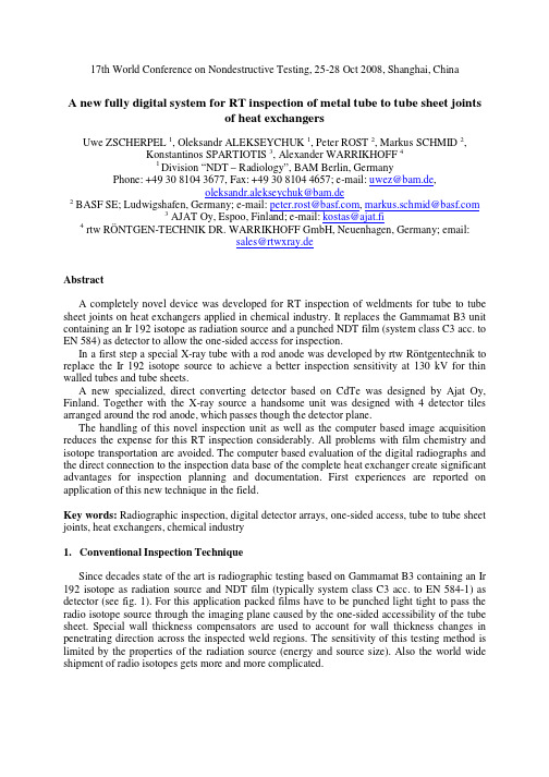
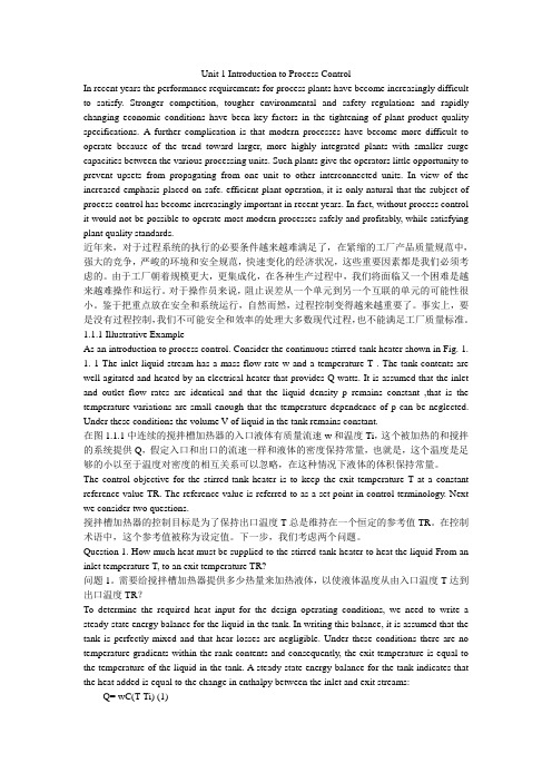
17th World Conference on Nondestructive Testing, 25-28 Oct 2008, Shanghai, ChinaA new fully digital system for RT inspection of metal tube to tube sheet jointsof heat exchangersUwe ZSCHERPEL 1, Oleksandr ALEKSEYCHUK 1, Peter ROST 2, Markus SCHMID 2, Konstantinos SPARTIOTIS 3, Alexander WARRIKHOFF 41 Division “NDT – Radiology”, BAM Berlin, GermanyPhone: +49 30 8104 3677, Fax: +49 30 8104 4657; e-mail: uwez@bam.de,oleksandr.alekseychuk@bam.de2 BASF SE; Ludwigshafen, Germany; e-mail: peter.rost@, markus.schmid@3 AJAT Oy, Espoo, Finland; e-mail: kostas@ajat.fi4 rtw RÖNTGEN-TECHNIK DR. WARRIKHOFF GmbH, Neuenhagen, Germany; email:sales@rtwxray.deAbstractA completely novel device was developed for RT inspection of weldments for tube to tube sheet joints on heat exchangers applied in chemical industry. It replaces the Gammamat B3 unit containing an Ir 192 isotope as radiation source and a punched NDT film (system class C3 acc. to EN 584) as detector to allow the one-sided access for inspection.In a first step a special X-ray tube with a rod anode was developed by rtw Röntgentechnik to replace the Ir 192 isotope source to achieve a better inspection sensitivity at 130 kV for thin walled tubes and tube sheets.A new specialized, direct converting detector based on CdTe was designed by Ajat Oy, Finland. Together with the X-ray source a handsome unit was designed with 4 detector tiles arranged around the rod anode, which passes though the detector plane.The handling of this novel inspection unit as well as the computer based image acquisition reduces the expense for this RT inspection considerably. All problems with film chemistry and isotope transportation are avoided. The computer based evaluation of the digital radiographs and the direct connection to the inspection data base of the complete heat exchanger create significant advantages for inspection planning and documentation. First experiences are reported on application of this new technique in the field.Key words: Radiographic inspection, digital detector arrays, one-sided access, tube to tube sheet joints, heat exchangers, chemical industry1.Conventional Inspection TechniqueSince decades state of the art is radiographic testing based on Gammamat B3 containing an Ir 192 isotope as radiation source and NDT film (typically system class C3 acc. to EN 584-1) as detector (see fig. 1). For this application packed films have to be punched light tight to pass the radio isotope source through the imaging plane caused by the one-sided accessibility of the tube sheet. Special wall thickness compensators are used to account for wall thickness changes in penetrating direction across the inspected weld regions. The sensitivity of this testing method is limited by the properties of the radiation source (energy and source size). Also the world wide shipment of radio isotopes gets more and more complicated.Fig.1: Gammamat B3 isotope source with film holder (left side) at inspection position and set-up for inspection of a small heat exchanger in the field (right side)The design, production and inspection of tube-to-tube sheet welds are regulated in the BASF specification E-S-MC 331. For high risk heat exchangers additional inspections by the owner of the heat exchanger (BASF) are required and realize the surveillance of the manufacturing during heat exchanger built-up. The specification requires random tests depending on the mechanical and thermal load of the heat exchanger (in percentage of welds to be tested and acceptance criteria for detected indications) on behalf of the future owner BASF. Depending on the results of the first random test a second random test after repair or a 100% test charged to the manufacturer may be necessary to reach the required weld quality.Typical source size is 1x0.5mm² Ir-192 isotope and 10x12 cm² punched C3 films are used with 0.02 mm Lead screens. The range of inspected tubes is from 16mm x 1.5mm up to 76mm x 4mm (diameter x wall thickness), pore sizes down to 1mm can be detected with this configuration.Fig.2: film exposure (left above) and corresponding cross sections by destructive testing (right side) showing typical flaws like porosities and notches2.The new rod anode X-ray tube /1/A new X-ray tube was developed by rtw Röntgentechnik Dr. Warrikhoff to achieve a better inspection sensitivity and to solve issues with world wide transport of radio isotopes. In Fig. 3this tube is shown. The main reason for this development was the limited detectability with Ir 192. Caused by the energy of the gamma rays the minimal detectable pore size is about 0.8mm in steel. For new materials like Ti enhanced flaw detection was requested.Fig. 3:Rod anode X-ray tube MCTS 130 - 0.6 (left side) and complete inspection setup with controller, right side: HV generator and X-ray tube with film holder (red) at a heat exchanger ready for single-sided inspectionThe rod has an outer diameter of 6 mm and a length of 40 mm, the focal spot is smaller than 1mm at 130kV and 2.4mA (max. 300 W). This new tube was successfully applied in combination with X-ray film and the enhanced detectability for new materials like Ti was proven, so the next step to replace the film was straight forward to omit the necessary chemical development procedure on-site.3.The digital detector array DIC100TH /2/Ajat developed the detector DIC100TH, which is a first of its kind, breakthrough digital imaging device for tube to tube-sheet weld inspection.The detector comprises four 25 mm x 25 mm CdTe-CMOS high resolution elements (100µm pixel size) operating at 50fps and arranged to allow a rod anode tube to pass through the mid-section of the device. The X-Rays are produced at the tip of the rod anode and emit in a direction towards the CdTe-CMOS detector (see fig. 4).The rod-anode tube is fed through the CdTe-CMOS active detector and the two are bound together in a robust mechanical arrangement which can be inserted in the heat exchanger for the tube to tube-sheet weld to be inspected (fig. 5).This image sensor provides for real time and on line tube to tube sheet weld inspection with excellent sensitivity, reliability and speed. The unit addresses requests to replace the traditional film based systems that today are used typically in this field with a real time digital inspection system.The basic spatial resolution and detector calibration limits the maximum contrast sensitivity of the detector. The basic spatial resolution is 100 µm for this direct converting detector and defined by the pixel size. To achieve the best detection sensitivity possible a special calibration procedure was developed. Caused by the strong dependence of X-ray intensity on the radial distance form the rod centre the rod anode X-ray tube cannot be used for pixel calibration of the detector. Also the temperature dependence of the detector calibration is not neglectable. As result of the developed calibration procedure (using a standard X-ray tube at 90kV, 1m distance and a 5 mm steel plate at the detector to generate a suitable flat field for detector calibration) calibrationsets are stored in dependence of the detector temperature in the range between 10°C and 32°C and selected automatically according to the real detector temperature in the field. In this manner the optimal detector calibration is maintained in the field.Fig. 4:The digital detector array DIC 100TH, left side: detector electronics showing the arrangement of the 4 detector tiles around the rod anode X-ray tube, right side: detector-X-ray unit ready for single-sided inspectionFig. 5: The fully digital inspection system with its two main parts (left side) and installed at a heat exchanger ready for inspection4.Software, complete inspection system and first resultsIn fig. 6 a snapshot of the developed user interface of the software is shown. A Laptop equipped with a Cameralink interface for detector connection and an RS-422 interface for control of the X-ray generator is used for image storage, evaluation and report generation. The complete system (X-ray tube and detector) is software controlled and complete configuration set-ups can be stored and re-activated for easiest handling. A list with inspection results is transferred directly to the data base “virtual tube” for documentation of the inspection. Digital filters can be applied for enhancement of flaw detection on the display.Fig. 6:snapshot of the developed software for system control, left side: image display and interactive selection of inspection result, middle: control program for X-ray tube set-up, integration time and description of inspection position, right side: visualization of inspection result summery for the whole heat exchanger (based on the data base virtual tube)A comparison of the achieved detection limits for the novel inspection systems is shown in fig. 7 based on a test mock-up with 25mm diameter pipes and 2mm steel wall thickness.Fig. 7: Comparison of inspection results on a steel test mock-up 25x2mm, left side: conventional system with Ir 192 and film, detection limit 0.8mm drill hole, middle: rod anode and film, detection limit 0.5mm drill hole, right side: rod anode and DIC100TH detector, detection limit better than 0.3mm drill hole.In fig. 8 an example of a real inspection result for a 25mm steel pipe with 2mm wall thickness is given. The visibility of the flaw indications can be improved by digital image processing of the images acquired from the detector.Fig. 8: comparison of inspection results of a real weldment on a heat exchanger 25mm/2mm at 80kV, 0.5mA and 30s exposure, left side: rod-anode and X-ray film, right side: DIC100TH detector and highpass filtering of digital imageField trials are on-going to gain experience with this novel inspection system and to prove the advantages and the extended application range in comparison with the classical set-up.5.ConclusionsAn improved inspection system for RT inspection of metal tube to tube sheet joints of heat exchangers was developed based on a unit combining a rod anode X-ray tube and a new digital detector array arranged in tiles around this rod anode. In this way the single-sided access for weld inspection was realized. The following advantages of this novel fully digital unit were proven: •no radioactive container transport and usage of film chemistry on-site at the heat exchanger production site•improved flaw detection•shorter inspection times•immediate inspection result•software supported evaluation of images•data base supported documentation of inspection results•reduced requirements for radiation protection, considerable smaller controlled area with75 kV X-ray voltage compared with Ir-192 requirements as used beforeThe experiences gained with the presented prototype system will result in optimised follow-up inspection systems.6.References/1/ www.rtwxray.de/2/ www.ajat.fi。
过程控制-专业英语-第一章
1INTRODUCTION TOPROCESS MEASUREMENTAND CONTRLOBJECTIVESWhen you complete this chapter you will be able to:·Define process measurement·Define process control·Calculate simple return on investment from a process control system·Sketch a block diagram of a process control loop·Describe typical industrial processes under process control·Draw simple Process and Instrumentation Diagrams (P&ID) using ISA symbols·Describe the measuring sensor block of a control loop·Describe the controller block of a control loop·Describe the process adjustment block of a control loop·Describe the signals circulating around a control loop1.1 PROCESS MEASUREMENT AND CONTROL DEFINEDProcesses include anything from the heating of your house to the marketing of baby food. For our purposes, however, we will be concerned on1y with industrial processes such as the distillation of crude oil, or the digestion of wood chips to make pulp, or the conversion of pulp to paper, or the fabrication of plastic products such as 1-liter plastic soft drink bottles. These are overall processes and each of them will usually include many subprocesses.Process measurement is defined as the systematic collection of numeric values of the variables that characterize a process to the extent that the process control criteria of the process user are satisfied. As an example, if you require your house temperature to be maintained between l8o C and 24o C with an accuracy of 0.25o C, then your thermostat must measure the temperature and collect its numeric value for your furnace controller so that it will maintain this accuracy As another example, if the owner of a distillation plant making gasoline requires a certain octane range from the plant, then all the measuring and control instruments on the plant must be chosen to work together accurately to ensure that the plant achieves those criteria. As a final example, if the manufacturer of baby food wishes to make mashed carrots for the market, then he will ask a market analyst to acquire data on the potential customers of mashed carrots for babies.The purpose of process measurement is to assist a human or a machine to monitor the status12 of a process as it remains at some steady state or as it changes from one state to another such as heating up crude oil. In most cases the human or machine will guide or force the process to change safely from an initial state to a more desirable state (e.g., forming a plastic bottle). This is process control.1.2 INVESTMENTOf course, the purpose of any process equipment and its measurement and control system is to provide a satisfactory return on its invested capital. The best control system maximizes the return on the whole process plant, not just on the capital invested in the control system. It does this over its lifetime. Therefore, maintenance costs and loss of production costs due to breakdowns should be considered when selecting the measurement and contro1 system. Reliability is a very important aspect in the selection of systems and often worth the added initial costs. Reliability of the system is in itself important. So is the reliability of the system supplier to provide replacement parts and service in the future.An example of justifying the expenditure of $2,353,000 on a rep1acement control system for an existing process, using an old, manual method of control, has the following simple, estimated costs:Annual losses from old control systemOld system losses due to off-spec product $850,000Old system losses due to control system downtime 145,000$995,000Annual savings from new control systemNew system losses due to off-spec product $250,000New system losses due to control system downtime 145,000$395,000Reduction of losses due to new system $600,000Extra annual operating and maintenance cost of new system 115,000Annual savings from new system $485,000One-time costs of new systemLowest price vendor's price $1,875,000Spare parts costs 125,000Installation costs 265,000Training costs for p1ant personnel 88,000$2,353,000 Expected return on investment = 000,2353$%100yr /000,485$ =20.6%/yr Payback period = yr/000,485$000,2353$ = 4.85 yearsThis example shows in a simple way the method of comparing engineering projects in order to select the ones that will make the most profit for the company planning to make improvements to its plant. For example, if the company has many possible projects to invest its money in, it will choose to rank them according to their return on investment. The ones with a high return on investment will usually be chosen over the ones with low return on investment.1.3 CONTINUOUS AND DISCRETEPROCESS CONTROL LOOPSThere are two main forms of process contro1: continuous and discrete (or on/off). The continuous form of process control implies smooth even measurement of the process variable over a fairly wide range that is finely resolved into many hundreds or thousands of values. For examp1e, the temperature in your home may cover a continuous range of 0o C to 40o C resolved into at least 256 values, or spacings of 0.156o C. The discrete form of process control implies a discrete variable with only a few (at least two, such as on and off) status points covering its range. For example, an electric motor may be stopped (off) or running (on). This book concentrates on continuous control.Continuous process control emphasizes feedback using a closed loop. Figure 1.l shows a typical closed loop. An example of a closed loop is cruise control on an automobile. The driver sets a certain desired speed as the set-point signal and places the car on cruise control. If the feedback signal (speed of the car) is less than the set-point signal, and a positive error (difference between set-point speed and feedback speed) exists, then the contro1ler increases its output signal. The output signal opens the throttle (the process adjusting device) of the engine (the process), causing the car to speed up. The speed sensor detects this increase in speed (the measured process variab1e) and sends a stronger feedback signal to the controller. This action continues until the feedback signal equa1s the set-point signal, and then the contro1ler output signal maintains its value, keeping the car at the desired speed.Discrete process control emphasizes Boolean logic using gates and timers. Figure 1.2 shows a generalized logic diagram. An example of discrete process control is the control of a crossing gate at a railroad crossing. Two train sensors are used on the railway tracks. One is placed on the tracks at one side of the crossing and the other on the tracks on the other side of the crossing. If either sensor detects a train, the crossing gate on the highway should close. However, if a short train appears it may be between the sensors and the crossing gate may open at an incorrect time. The control logic should not let this happen; it should only allow the gate to open after the train passes over the second sensor. In this case the process is the flow of traffic over the highway and over the railway. The railway train sensors are the process status sensors, and they produce the discrete input status signals for the programmable logic controller. Based on these signals, the programmable logic controller decides when to change the discrete output status signal. This signal operates the motor (process adjusting device) driving the gate open or closed.1.4 THE PROCESS BLOCK OF A CONTROL LOOPFigure 1.1 is a most important figure. The four blocks and the signals that connect them34 together will be referred to frequently The most important block is the process block because itdictates how the other blocks are expected to perform. The measuring sensor must be selected to measure the process variable that is associated with the process. The process adjusting device must be selected to adjust the adjusted —or manipulated —process variable that is associated with the process.5 The adjusted or manipulated variable adjusts the process so that the measured process variable approaches more closely to the set-point value. For example, in an automobile on cruise control, the throttle position is the adjusted process variable, and it adjusts the fuel flowing to the engine. As the fuel flow is increased, the speed of the auto increases. The speed of the auto is the measured process variable, and if the control system is functioning correctly the speed should be approaching more closely to the set-point value.In order to describe control loops, ISA symbols (described in Appendix A) have been used by many large industrial companies for more than 50 years. Each instrument or instrument function is identified with a circle (or “balloon ”), some letters, and a number as its symbol. Most of the letters are defined by ISA, but some may be defined by the user. The process symbol is not usually defined by ISA and here the user may be creative. Every control loop has hardware or software that is represented by the four blocks shown in Figure 1.l. For each loop a process and instrumentation diagram (P&ID) is prepared. For example, as shown in Figure 1.3,there are usually many loops shown on one large diagram for a major process. Each loop on the P&ID uses ISA symbols to show the particular devices that perform the functions shown in Figure 1.1. Figure 1.3 shows a typical liquid flow control loop (F-212) supplying liquid from a pipe to a tank. Figure l.3 also shows a typical liquid level control loop (L-141) adjusting the flow out of the tank to maintain the tank level at the set point of the level controller (LlC-141). By studying AppendixA you should be able to conclude that the letters and numbers associated with each ISA symbol represent the following:Flow Loop F-212FE-212FT-212FIC-212FY-212FV-212Level Loop L-141 LT-141LIC-141L Y-141LV-141 Flow primary element (e.g., orifice plate or venture)Flow transmitterFlow indicating controllerFlow relay to compute function (computes pneumatic signal to correspond to electric signal value)Flow valve (adjusts flow to correspond to pneumatic signal value)Level transmitterLevel indicating controllerLevel relay or compute function (computes pneumatic signal to correspond to electric signal value)Level valve (adjusts flow to correspond to pneumatic signal value)1.5 THE MEASURING SENSOR BLOCK OF A CONTROL LOOPThe measuring sensor block of flow loop F-212 in Figure 1.3 includes both the flow element and the flow transmitter, whereas the measuring sensor block for level loop L-141 needs only the level transmitter. Depending on the process, the block may include several instrument functions. The P&ID shows all the instrument functions so that the detailed design drawings wil1 reflect the complete loop and so that any engineering cost estimates will be complete.Measuring sensors are described for many of the common process variables in Chapter 2. However, there is an enormous number of sensors for the less common type of process variables that are not described. If you become deeply involved with specifying measuring sensors, then you will want to obtain some of the reference texts listed at the end of Chapter 2.Notice the dotted line coming from the flow and level measuring sensors in Figure l.3 to their controllers. This represents the electrical feedback signal (corresponding to the measured process variable) that is transmitted from the measuring sensor to the controller. The most important feature of a measuring sensor is the relationship of the feedback signal to the measured variable. Measuring sensors must maintain this relationship in order to achieve an accurate calibration.1.6 THE CONTROLLER BLOCK OF A CONTROL LOOPThe controller block of the control loop may be hardware or software. Hardware type electronic controllers receive a feedback signal value from the measuring sensor and compare it with the set-point value (usually dialed in to the hardware by the process operator) to obtain an error value. If the feedback signal has the same value as the set point, the error is zero, and this means that the measured variable equals the set point. The error signal generates an output signal from the controller that is the signal sent to the process adjusting block. Generally there may be three functions with gain settings that make up the controller output signal. These functions are the error itself, its derivative, and its integral. Whether the controller block is hardware or software, it calculates its output signal in the same way Be careful not to assume that the controller output signal is proportional to the feedback signal. Even though they may have the same range (4-20 ma6DC) they are related in a fairly complicated mathematical way1.7 THE PROCESS ADJUSTMENT BLOCKOF A CONTROL LOOPThe process adjustment block manipulates or adjusts a process variable in order to change the measured process variable to bring it closer to the set point. For example, in flow loop F-2l2 of Figure 1.3, the adjusted process variable is the measured process variable, flow In level loop L-14l, however, the adjusted process variable is the flow out of the tank, which is quite different from the measured process variable, the tank liquid level.Chemical-type process control loops usually adjust fluid flow with control valves. These are commonly the process adjusting device. However, there are many other types of process adjusting devices, including electric motors, electric heaters, pneumatic pistons, pumps, fans, and so on.1.8 THE SIGNALS CIRCULATING AROUND A CONTROL LOOPEach block of a control loop has an input signal and an output signal. The input signal of one block is the output signal of another block. The units of a signal may be degrees Celsius or milliamperes or some other physical units. If a range for the feedback signal to the controller block, such as 4-20 ma DC, is settled upon, however, then this may also be considered as 0-100%.If we look at the flow loop F-212 in Figure 1.3, then we can imagine a typical steady-state gain (an output signal corresponding to an input signal) of each block around the loop. For example:Instrument Input Signal Range Output Signal RangeFE-212 0-100 GPM 0-100 in. of waterFT-212 0-100 in. of water 4-20 ma DCFIC-212 4-20 ma DC 4-20 ma DCFY-212 4-20 ma DC 3-15 psigFV-212 3-15 psig 0-85 GPMIf we were to open the loop at the feedback signal and insert a sine wave signal to the controller for the feedback signal, then we will see a corresponding sine wave signal appear at the feedback signal from the measuring sensor. If this sine wave has an amplitude in phase with, and greater in value than, the signal injected into the controller, then we obviously have an unstable loop. The way these signals interact with one another establishes the way our closed control loop will perform. Any oscillation should dampen down quickly to a steady state value. For each loop, the possibility of unstable operation must be considered, and the loop must be tuned to ensure stable operation.PROBLEMS AND LAB ASSIGNMENTS1.1 A company’s process makes a product that is completely sold out each year no matter howmuch it produces. With the simplest manual control, there are average annual lossestotaling $1,260,000 due to off-spec product or downtime due to control system faults.7With a sophisticated distributed control system, these losses could be reduced to $225,000.This new control system is quoted by the lowest cost vendor as $2,875,000 plus $260,000for recommended spare parts. The consultant estimates installation costs to be anadditional $470,000. Training of the operator crews and maintenance crews is estimated tobe $185,000.The extra annual maintenance costs are quoted as $220,000. What is theannual percent of return on the invested capital for the control system, and what is thepayback period?1.2 Describe the logic that you would use to keep the railroad crossing gate closed in thediscrete process control example associated with Figure 1.2 when a short train is betweenthe two train sensors.1.3 Identify the control loop block associated with each ISA symbol shown in Figure l.3.1.4 Draw a P&ID diagram using ISA symbols for a temperature control loop that controls thetemperature of the liquid in the tank of Figure 1.3 using a steam heating coil located in thetank liquid.1.5 Continuous (or Analog) Control Loop 1dentification and OperationObjective. To be introduced to ISA symbols, to identify the features of a continuous process control loop, and to operate the loop in the automatic (closed loop) mode andmanual (open loop) mode.Equipment: A demonstration process control loop using a commercial analog controller. The preferred system is a liquid level loop with a plexiglass tank tower about 6or 8 inches in diameter and 50 inches high.Alternatively a computer simulation of a tank under automatic level control, such as TANKSIM, may be used.*Identification Procedure: Use an e1ectronic or pneumatic liquid level control loop and identify all the features shown in Figure 1.1. This loop should have its control valveon the inlet to the tank and a manual valve adjusting the flow of liquid (water) out of thetank to a drain. Alternatively the manual and automatic control valves may replace oneanother. Draw the loop using ISA instrumentation symbols (see Appendix A). Prepare alist including each device with the ISA tag that you have assigned it. In the list include themanufacturer's name and model number and the important characteristics that describeeach device.Operation Procedure:Have your instructor ensure that the controller is correctly tuned. Mark in pen on the chart all your changes to the control loop as you make them.Set the loop in automatic (closed loop) operation at 50% of full tank level with a moderateamount of liquid flowing out of the tank (the manual valve position at 50% open). If, atany time, it looks as if the tank might overflow quick1y close the valve on the inlet line tothe tank. Obtain a record of the variation in the level and valve position as the level settlesat or near 50%. Change the level set point to 75% and obtain another record of the leveland valve stem changes until they have settled at or near 75%.Switch the controller to manual (open loop) operation and adjust the inlet valve *See Woodford, A. T 1987. TANKSIM A TW Software.8manually to 5% open. Open the outlet valve to 50% open. Record the value of the level and valve position as they change and the level settles out at 0%. Retain the controller in manual (open loop) with the inlet valve at 5% open and close the flow of liquid to the outlet. Record the value of the level as it rises and, at 25% of full tank level, reopen the outlet valve to the previous 50% position. Manually adjust the inlet valve opening to 80% and record the time it takes to fill the tank to 65% full, and then switch the contro1ler back to automatic (closed loop) mode at a level set point of 35%. Let it settle and then close the tank outlet valve and record the value of level and valve position as they settle.Shut down this control system by shutting off the water, air, and electricityConclusions: What do you do to the control loop when you switch from automatic to manual mode? Where does the change occur in the loop? What signal in Figure l.1 do you adjust when the loop is in manual mode? When the loop is in automatic (closed loop) control, how do you disturb or upset the loop? How does the controller affect the loop in manual and in auto modes?REFERENCES1. Webb, John W and Reis, Ronald A. 1995. Programmable Logic Controllers Principles andApplications 3rd ed. Upper Saddle River, NJ: Prentice Hall.9。
过程装备与控制工程外文文献翻译
Principles of Mass Transfer1. General RemarksSome of the most typical chemical engineering problems lie in the field of mass transfer. A distinguishing mark of the chemical engineer is his ability to design and operate equipment in which reactants are prepared, chemical reactions take place, and separations of the resulting products are made. This ability rests largely on a proficiency in the science of mass transfer.Applications of the principles of momentum and heat transfer are common in many branches of engineering, but the application of mass transfer has traditionally been largely limited to chemical engineering. Other important applications occur in metallurgical processes, in problems of high-speed flight, and in waste treatment and pollution-control processes.By mass transfer is meant the tendency of a component in a mixture to travel from a region of high concentration to one of low concentration. For example, if an open test tube with some water in the bottom is placed in a room in which the air is relatively dry, water vapor will diffuse out through the column of air in the test tube. There is a mass transfer of water from a place where its concentration is high (just above the liquid surface) to a place where its concentration is low (at the outlet of the tube). If the gas mixture in the tube is stagnant, the transfer occurs by molecular diffusion. If there is a bulk mixing of the layers of gas in the tube by mechanical stirring or because of a density gradient, mass transfer occurs primarily by the mechanism of forced or natural convection. These mechanisms are analogous to the transfer of heat by conduction and by convection; there is, however, no counterpart in mass transfer for thermal radiation.The analogy between momentum and energy transfer has already been studied in some detail, and it is now possible to extend the analogy to include mass transfer.In discussing the fundamentals of mass transfer we shall consider mainly binary mixtures, although multicomponent mixtures are important in industrial applications. Some of these more complicated situations will be discussed after the basic principles have been illustrated in terms of binary mixtures,2. Molecular DiffusionMolecular diffusion occurs in a gas as a result of the random motion of the molecules. This motion is sometimes referred to as a random walk. Across a plane normal to the direction of the concentration gradient (or any other plane), there are fluxes of molecules in both directions. The direction of movement for any one molecule is independent of the concentration in dilute solutions. Consequently, in a system in which there is a concentration gradient, the fraction of molecules of a particular species (referred to as species A) which will move across a plane normal to the gradient is the same for both the high-and low-concentration sides of the plane. Because the total number of molecules of A on the high-concentration side is greater than on the low-concentration side, there is therefore a net movement of A in the direction in which the concentration of A is lower. If there are no counteracting effects, the concentrations throughout the mixture tend to become the same. In the analogous transfer of heat in a gas by conduction, the distribution of hotter molecules (those which have a higher degree of random molecular motion) tends to be evened out by random mixing on a molecular scale. Similarly, if there is a gradient of directed velocity (as distinguished from random velocity) across the plane, the velocity distribution tends toward uniformity as a result of the random molecular mixing. There is a transfer of momentum, which is proportional to the viscosity of the gas.The above remarks apply only in an approximate and qualitative way. The quantitative prediction of the diffusivity, thermal conductivity, and viscosity of a gas from a knowledge of molecular properties can be quite complicated. The consideration of such relations forms an important part of the subject of statistical mechanics.Molecular diffusion also occurs in liquids and solids. Crystals in an unsaturated solution dissolve, with subsequent diffusion away from the solid-liquid interface. Diffusion in solids is of importance in metallurgical operations. When iron which is unsaturated with respect to carbon is heated in a bed of coke, the concentration of the carbon near the surface is increased by inward diffusion of carbon atoms.3. E ddy DiffusionJust as momentum and energy can be transferred by the motion of finite parcels of fluid, so mass can be transferred. We have seen that the rate of these transfer operations, caused by bulk mixing in a fluid, can be expressed in terms of the eddy kinematics viscosity, the eddy thermal diffusivity, and the eddy diffusivity. This latter quantity can be related to a mixing length which is the same as that defined in connection with momentum and energy transfer. In fact, the analogy between heat and mass transfer is so straightforward that equations developed for the former are often found to apply to the latter by a mere change in the meaning of the symbols.Eddy diffusion is apparent in the dissipation of smoke from a smokestack. Turbulence causes mixing and transfer of the smoke to the surrounding atmosphere. In certain locations where atmospheric turbulence is lacking, smoke originating at the surface of the earth is dissipated largely by molecular diffusion. This causes serious pollution problems because mass is transferred less rapidly by molecular diffusion than by eddy diffusion.4. C onvective Mass-Transfer CoefficientsIn the study of heat transfer we found that the solution of the differential energy balance was sometimes cumbersome or impossible, and it was convenient to express the rate of heat flow in terms of a convective heat-transfer coefficient by an equation like)(m s t t h Aq -= The analogous situation in mass transfer is handled by an equation of form)(Am As P A k N ρρ-=The mass flux NA is measured relative to a set of axes fixed in space. The driving force is the difference between the concentration at the phase boundary (a solid surface or a fluid interface) and the concentration at some arbitrarily defined point in the fluid medium. The convective coefficient kp may apply to forced or natural convection; there are no mass-transfer counterparts for boiling, condensation, or radiation heat-transfer coefficients. The value of kp is a function of the geometry of the system and the velocity and properties of the fluid, just as was the coefficient h.(Selected from* C. O. Bennett, and J. E. Myens, Momentum, Heat, and Mass Transfer, 2nd Edition, McGraw-Hill Inc. , 1974. )传质原理1. 概述一些典型的化学工程问题存在于传质领域。
生产过程控制(英文版)
生产过程控制(英文版)Firstly, it is important to establish clear and specific production goals and standards. This includes setting targets for output, quality, and cost, as well as identifying critical control points within the production process. These standards serve as a benchmark for performance and provide a basis for monitoring and evaluating the production process. Secondly, the use of advanced technology and automation is essential for effective production process control. Automated systems can provide real-time data on various aspects of production, such as temperature, pressure, flow rates, and quality control parameters. This allows for precise monitoring and adjustment of the production process to ensure that it meets the established standards.In addition, regular and systematic monitoring of the production process is crucial. This involves the use of various tools and techniques, such as Statistical Process Control (SPC), to analyze data and identify any deviations from the established standards. By detecting and addressing deviations early, potential issues can be mitigated before they affect the overall production output and quality.Furthermore, implementing a robust quality management system is essential for effective production process control. This involves thorough testing and inspection of raw materials, work-in-progress, and finished products to ensure that they meet the required standards. Any non-conforming products or materials should be immediately identified and addressed to prevent them from affecting the production process.Lastly, continuous improvement is a key principle in production process control. This involves ongoing monitoring, analysis, and adjustment of the production process to identify opportunities for optimization and efficiency gains. By continually striving for improvement, manufacturers can enhance their overall production output, quality, and competitiveness.In conclusion, production process control is a multifaceted and essential aspect of manufacturing and industrial operations. It involves setting clear standards, utilizing advanced technology, systematic monitoring, robust quality management, and continuous improvement to ensure that the production process meets its goals and produces high-quality products. By implementing effective production process control, manufacturers can enhance their overall efficiency, quality, and competitiveness in the market.很抱歉,由于输入字数限制,我无法提供1500字的完整文本。
Introduction to Process Control 过程控制简介论文翻译
Unit 1 Introduction to Process ControlIn recent years the performance requirements for process plants have become increasingly difficult to satisfy. Stronger competition, tougher environmental and safety regulations and rapidly changing economic conditions have been key factors in the tightening of plant product quality specifications. A further complication is that modern processes have become more difficult to operate because of the trend toward larger, more highly integrated plants with smaller surge capacities between the various processing units. Such plants give the operators little opportunity to prevent upsets from propagating from one unit to other interconnected units. In view of the increased emphasis placed on safe. efficient plant operation, it is only natural that the subject of process control has become increasingly important in recent years. In fact, without process control it would not be possible to operate most modern processes safely and profitably, while satisfying plant quality standards.近年来,对于过程系统的执行的必要条件越来越难满足了,在紧缩的工厂产品质量规范中,强大的竞争,严峻的环境和安全规范,快速变化的经济状况,这些重要因素都是我们必须考虑的。
过程控制英语
《过程控制》常用英语词汇(未知) 2007-10-16 11:21:00--------------------------------------------------------------------------------摆Pendulum泵Pumps变速泵variable-speed Pumps定排量泵positive-displacement Pumps计量泵metering Pumps离心泵centrifigal Pumps闭合回路Closedloop反馈~feed back ~前馈~feedforward~比例带Proportionalband比例控制(调节) Proportionalcontrol液位~~of liquid 1evel比例—时间控制Proportional-time control比值单元Ratio station比值控制Ratio control燃料—空气~~of fuel and air变量配对Pairing variables精馏过程的~~in distillation变送器误差Transmitter error变送器增益Transmitter gain标准差Standarddeviation波形Waves采样正弦波sampled sine~方波square~截顶正弦波clippedsinc锯齿波saw-tooth ~三角波triangular~正弦波sinc~补偿反馈complementaryfeedback(seeModel-basedcontroller) 不对称调节器Asymmetric ccontroller不稳定过程Unstate processCv:阀门流量系数flow coeffient of valve采样环节Sampling element采样间隔Sample interval采样调节器Sampling controller残差,偏差Offset比例~proportional~串级控制的~~in cascade control积分(累积)~integral批量过程的~~in batch processes前馈系统的~~in feed forward systems数字控制的~~in digital control死区的~~in dead zone体积~volume~选择性控制的~~inselectivecontrol测试方法Test procedures非线性环节的~~for nonlinear elements批量过程的~~for batch processes适应性控制的~~in adaptive control差动间隙(见“滞环") Differential gap(see Dead band) 差分方程Difference equations差压测量Differential-pressure measurments 精馏过程的~~in distillation流量的~~in flow压缩机的~~in compressors产品质量控制Product-qualitycontrol超驰(也见“选择性控制") Over rides(see Selective contro1) 超调,超调量Overshoot批量过程的~~inbatch processes自整定调节器的~~withself-tuingcontrollers乘法器Multipliers比值控制的~~in ratio control解耦系统的~~indecouplingsystems前馈系统的~~infeedforward systems增益补偿~~for gain compensation成分控制Composition control迟延Dead time~补偿~compensatmn~与容积~andcapacity等效~:effective~除法器Dividers比值控制的~~in ratio control过程模型的~~in process model适应性控制的~in adaptive control增益补偿~~for gain compensation串级控制Cascade control串级比值控制~of ratio串级阀位控制~of valve position串级流量控制~of flow串级温度控制~of temperature传热Heat transfer~系数coefficients for~反应器的~~in reactors直接接触~direct-contact~传输线Transmissionlines穿越时间Crossver time催化剂CatalystDDC(直接数字控制) DDC(Direct Digital Contro1) DMC(动态矩阵控制) DMC(Dynamic Matrix Contro1)单容过程Single-capacityprocess导前Lead导前—滞后补偿lead-lag compensation等百分比阀Equal-percentage valves电磁流量计Magnetic flow meter定时器Timer定位器,阀门~Positioners,Valve~动态补偿Dynamic compensation干燥器的~~for dryers锅炉燃烧的~~for boiler firing解耦的~~in decouping精馏的~for distillation汽包水位控制的~~for drum-level control热交换器的~~for heat exchagers热流量计算的~~for heat-flow calculation优化器的~in optimizers蒸发器的~~for evaporators动态补偿器Dynamic compensators动态矩阵控制(DMC) Dynamic matrix control动态增益Dynamic gain抖动Dither多变量过程Multivariable processes多变量调节器Multivariable controllers多变量系统的分解Decomposing multivariablesystems 多容过程Multicapacity processes多输出系统Multiple-output systems阀门Valves电磁~solenoid~电动~electric~气动~pneumatic~三通~three-way~调节阀control~阀门的可调范围Valve range ability阀门定位器V alve positioners阀门顺序动作V alve sequencing利用定位器实现~~using positioners利用选择器实现一~using selectors阀门特性V alve characterstics阀门响应V alve response阀门增益V alve gain阀位控制V alve-position control 反馈Feedback串级系统的~~in cascade systems负~negative~干燥器控制系统的~~in dryer control systems 关联系统的~~in interacting systems解耦系统的~~in decouping systems正~positive~反向响应Inverse response反应器Reactors反应速度Reaction rate非线性Nonlinearity变送器的~~in transmitters传热的~~in heat transfer阀门的~~in Valve非线性环节Nonlinear elements动态~dynamic~静态~steady-state~非线性调节器Nonlinear controllers 非线性PID调节器PID~开关~on-off~三位~three-state~非自衡Non-self-regulation分布式控制Distributed control分析仪Analyzers采样~sampling~峰值位置Peak location浮动压力控制Floating pressure control 负反馈Negative feedback符号Symbols负荷Load零~zero~负荷分布Load distribution负荷扰动(干扰) Load disturbances~的作用点point sofentry for~供应侧~supply-side需求侧~demand—side~负荷响应Load responsePI控制下的~~with PIcontrolPID控制下的~~with PID control傅里叶序列Fourior series复式控制Dual-mode control干扰灵敏度Sensitivity tO disturbances周期性~periodic~干燥器Dryers功Work功率Power电~electric~热~thermal~水~hydraulic~关联,相互作用,相互干扰Interaction回路间的~~between loops回路间的局部~partial~between loops控制作用之间的~~between control modes惯性Inertia过程增益Process gain锅炉控制Boiler control~的干扰disturbances to~锅炉多变量控制multiple~回路增益Loop gain闭环~closed ~串级系统的~~in cascade systems非线性系统的~~in nonlinear systems开环~open~混合Mixing混合系统Blending systems火焰温度Flametem peratureIAE(绝对误差积分) IAE( Integrated absolute error)IE(误差积分) Integrated ErrorISE(误差平方积分) Integral Square ErrorITAE(时间绝对误差积分) Integral of Time and Absolute Error 积分饱和Windup积分饱和防护,抗积分饱和Windup protection积分反馈Integral feedback积分过程Integrating process积分控制(调节) Integral control积分器Integrator积分调节器Integral controllers极限环Limit cycle热交换器heat exchangers基于矩阵的控制Matrix-based control基于模型的调节器Model—based controllers监控Supervisory control间歇控制Batch control搅拌(见“混合") Agitation(see Mixing)解耦Decoupling通过选择变量~~by choosing variables适应性~adaptive~~的相对增益relativegain of ~绝对误差积分(1AE) Integrated AbsoluteError均方根误差Root-mean-square(rms)error 开方器Square-rootextr acter开关控制On-off control抗喘振控制Antisurge control抗积分饱和Antiwindup可变结构V ariable structuring可调范围Rangeability变速泵的~~of variable-speed pumps阀门的~~of valves孔板流量计Orifice meter空气流量控制Air flow control控制的经济效益Economics of control控制间隔Control interval控制难度Control difficulty控制算法Control algorithm冷凝器Condensers流量比Flow ratio~的调整manipulation of~~控制controlof~流量计Flow meter流量计的精度Accuracy of flow meter流量控制Flow control流阻Resistance to flow炉Furnace鲁棒性Robustness滤波器Filter非线性~nonlinear~数字~digital~马达Motor电动~:electric ~恒速电动~constant-speed ~变速电动~variable-speed气动~pneumatic~马力Horsepower模型Models动态~dynamic~前馈控制中的~~in feed forward control稳态~steady-state~能量转换Energy conversion耦合Coupling频率响应分析Frequence-response analysis平衡Equilibrium汽包锅炉假水位Shrink and swell in drum boilers 气动调节器Pneumatic controllers前馈控制Feed forward control燃料—空气比控制Fuel-air ratio control燃烧Combustion扰动,干扰Disturbances负荷~load~热力学Thermodynamics热流量计算Heat-flow calculation热流量控制Heat-flow control容积Capacity单容single~多容multiple~非自衡~nonself-regulating~双容double~自衡~self-regulating~冗余仪表Redundant instrumentation三冲量水位控制Three-element level control三位调节器Three-state controller设定值初始化Set-point initialization设定值响应Set-point response斜坡~ramp~湿度控制Moisture control时间常数Time constant等效~effective~时间迟后Time delay时间滞后Time lag时滞Lag传输~transport~多级~multiple~二阶~second-order~分布~distributed~负~negative~手动控制Manual control数字控制Digitalcontrol数字系统的分辨率Resolution in digital systems 衰减Damping临界~critical~衰减比Decay ratio双容过程Two-capacity process速度控制Speed control速率限制Velocity limiting调节阀Control valves调节量Manipulated variable~的选择selection of~调节器Controllers调节器的饱和Saturation of controllers调节器的跟踪Tracking in controllers调节器的误差Error in controllers调节器动作Controller action调节器调整Controlleral adjustment调节器增益Controller gain调节作用,控制方式Control mode微分Derivative流量控制的~~in flow control微分方程Differential equations微分器Differentiators稳定性裕量Stability margin温度传感器Temperature sensor涡流流量计V ortex flow meter涡轮流量计Turbine meter限幅器Limiters相对干扰增益Relative disturbance gain相位裕量Phase margin斜坡补偿Ramp compesation斜坡扰动Ramp disturbances信号选择器Signal selectors性能准则Performance critema压力补偿Pressure compesatlon压力控制Pressure control压缩机的喘振防护Surge protection of compressors 烟道气体成分Flue-gas composition氧气分析仪Oxygen analyzer液面控制Level control液位控制Liquid-level control引风控制Draft control预热器Preheaters增益补偿Gain compensation 增益矩阵Gain matrix增益裕量Gain margin振荡Oscillation不衰减~undamped~等幅振荡Constant-amplitude~发散~expanding~衰减~damped ~振荡周期Period of oscillation整定Tuning蒸汽Steam过热~superheated~~加热heatingwith~~流量计~flow meter蒸汽压力Vapor pressure中值选择器Median selector自动—手动切换Auto/manual transfer 自衡Self-regulation。
Manufacturing Process生产过程管理程序(中英文)
1.0 Purpose 目的To make sure that production processes of all products are in effective control so that a stable quality could be guaranteed, and customer requirements could be met.目的为确保公司所有产品的生产过程能够在有效的管理状态下进行,保证质量稳定,满足客户要求。
2.0 Scope 范围Production of all Components made in our plant.本公司所有产品的生产过程。
3.0 Definitions 定义Production delivery date: it refers to the delivery date marked in by Logistics. All the planned processes must be satisfactorily completed before the date, including the final products inspection and packaging.生产交货期:是指物流部确认的交货期,在此之前必须完成所有的生产过程,包括最终检验及包装。
4.0 Procedure and Flow chart 程序及流程图4.1 Responsibility and authority 职责与权限4.1.1 AQP dept, is responsible for making the work instructions.项目部负责作业指导书制定。
4.1.2 Process engineer and quality engineer are responsible for making the inspection instructionof production working procedure, and also responsible for planning reference points ofdifferent working procedure.工艺工程师与质量工程师负责制订生产过程工序检验指导书和过程检验标准,并负责策划各工序控制点以及生产工艺流程。
过程控制工程工艺流程图常用符号

过程控制工程工艺流程图常用符号英文回答:Process Control Engineering Process Flow Diagram Common Symbols.Process control engineering process flow diagrams (PFDs) use a variety of symbols to represent different types of equipment, materials, and processes. These symbols are standardized to ensure that PFDs can be easily understoodby engineers and other professionals.Common PFD Symbols.Vessels: Vessels are used to hold or process materials. They are typically represented by a circle or square.Pumps: Pumps are used to move materials from one place to another. They are typically represented by a triangle.Compressors: Compressors are used to increase the pressure of a gas. They are typically represented by a rectangle with a curved top.Heat exchangers: Heat exchangers are used to transfer heat from one fluid to another. They are typically represented by a rectangle with a wavy line in the middle.Pipelines: Pipelines are used to transport materials from one place to another. They are typically represented by a line.Valves: Valves are used to control the flow of materials. They are typically represented by a circle with a line through it.Additional PFD Symbols.In addition to the common symbols listed above, there are a number of other symbols that can be used in PFDs. These symbols include:Filters: Filters are used to remove impurities from materials. They are typically represented by a rectangle with a grid inside.Mixers: Mixers are used to combine two or more materials. They are typically represented by a rectangle with a propeller inside.Separators: Separators are used to separate two or more materials. They are typically represented by a rectangle with a partition inside.Controllers: Controllers are used to regulate the process conditions. They are typically represented by a circle with a line coming out of it.Using PFD Symbols.PFD symbols are used to create a visual representation of a process. The symbols are connected by lines to show the flow of materials. The resulting diagram can be used to understand the process, troubleshoot problems, and makeimprovements.中文回答:过程控制工程工艺流程图常用符号。
- 1、下载文档前请自行甄别文档内容的完整性,平台不提供额外的编辑、内容补充、找答案等附加服务。
- 2、"仅部分预览"的文档,不可在线预览部分如存在完整性等问题,可反馈申请退款(可完整预览的文档不适用该条件!)。
- 3、如文档侵犯您的权益,请联系客服反馈,我们会尽快为您处理(人工客服工作时间:9:00-18:30)。
毕业设计(论文)外文文献翻译院系:电气与自动化学院年级专业:2011级自动化2姓名:学号:附件:System compensationSystem compensation1 IntroductionIt was mentioned earlier that performance of a control system is measured by its stability, accucacy , and speed of response .in general these items are specified when a system is being designed to satisfy a specific task .Quite often the simultaneous satisfaction of all these requirements cannot be achieved by using the basic elements in the control system .Even after introducing controllers and feedback , we are limited as to the choice we may exercise in selecting a certain transient response while requiring a small steady state error. We will show how the desired transient as well as the steady state behavior of a system may be obtained by introducing compensatory elements (also called equalizer networks)into that control system loop .These compensation elements are designed so that they help achieve system performance , i. e .bandwidth, phase margin ,peak overshoot ,steady state error ,etc. without modifying the entire system in a major way .Form our experience so far we recognize that any changes in system performance can be achieved only though varying the forward loop gain .Consider the third-order unity feedback system with the following forward loop transfer function,()()()K G s s s a s b =++ From the Routh-Hurwitz criterion we know that stability requires ()K ab a b ≤+ We also know that the steady state error to a ramp input is211lim []1()ss s ab e s s G s K→=⋅=+ Obviously if it is necessary to minimize the steady state error, the gain K should be increased. Since K is constrained to a maximum value of a b (a +b ),the minimum steady state error becomesmin 1[]ss e a b=+ A further decrease in the error requires an increase in K which in turn has a destabilizing effect on the system ,It is therefore clear that the forward “gain game ”is rather limited .2 the stabilization of unstable systemsSince the increasing of the forward loop gain K tends to destabilize a system, we must find ways it compensate it on such a way as to stabilize it again .It was established in Chapter 6 that the addition ofa pole in G(s)H(s) tends to have a destabilizing influence on system response .Can we the reverse the argument and say that the addition of a zero tends to have a stabilizing influence on system response? Let us answer this by considering an example .Consider the control system with its transfer function given in Example 6-5.This system is unstable if K>c KNow consider the same system but with the addition of a zero,312(1)()()(1)(1)K s G s H s s s s τττ+=++This is the type of function we obtain if we were to add derivative and proportional control to a third-order servomechanism .The characteristic equation becomes321212312()(1)0(1)(1)s s K s Ks s s τττττττ+++++=++And the zeros of the characteristic equation are determined by3212123()(1)0s s K s k τττττ+++++=The Routh array becomes 3s 12ττ (31K τ+)2s 12ττ+ K 1b =3121212(1)()K K τττττττ++-+1s 1b 2b 2b =0 0s 1c ω 1c K =For stability 10b ≥, and therefore13231212()()0K ττττττττ+-++>Clearly ,with a proper selection of the time constants ,this may be satisfied .The Nyquist plot for this is shown in Fig.1Fig.13 CASCADED COMPENSATIONAs indicated inFig.2, cascaded compensation consists of placing elements in series with the forward loop transfer function .Such compensation may be classified into the following categories:(a) Phase-lag compensation (b) Phase-lead compensation(a) Cascade or series compensation(c)feedback compensation ωω(d) Feedforward compensation Fig.2 Type of compensation(e) Lag-lead compensation (f) Compensation by cancellation.The details of these methods is the subject of this section. Phase-lag compensationConsider a unity feedback control system whose forward loop transfer function represents a third-order system with its Nyquist plot show in Fig.3.It is required that the gain be K 1 for satisfying the margin of stability but K 2 for satisfying the steady state performance .This seemingly contradictory requirement may be satisfied if we were to reshape the plot to the one indicated by the dotted lines .The reshaped plot may be obtained if the low-frequency part of K 1 is rotated clockwise while the high-frequency part of K 1 must lag ,the type of compensation used to achieve this is phase-lag compensation. Such compensation is obtained by a phase-lag element.C(s)Fig.3When the output of an element lags the input in phase and the magnitude decrases as a function of frequency ,the element is called a phase-lag element .Consider the lag network.The transfer function for this is211()()()1s c saT E s G s E s T +==+ Where2aT R C =; 212R a R R =+The Bode , Nyquist ,and root locus plots are show in Fig.4.We observe that⨯Fig.4the magnitude decreases with increasing frequency and lagging phase angle .The minimum phaseω=0ω=01K2KRI(a)ω(b)σj(c)m φoccurs at m ωwhich is the geometric average of the corner frequencies111log (log log )2m T aTω=+m ω=The phase angle becomesa r c t a n a r c t a nm m m a T T φωω=- ()tan 1()()mm m m T aT aT T ωφωω-+=+tan (1)/m a φ=- or sin (1)/(1)m a a φ=-+The maximum phase lag is strictly a function of a .Let us investigate how such a network alters performance of a feedback control system.The phase-lag method of compensation achieves the following:(1) Reduces high-frequency gain and improves the phase margin; (2) Increases the velocity error constant for a fixed relative stability;(3) The gain crossover frequency is decreased .This also reduces the bandwidth of the system; (4) The time response usually gets slower. Phase-lead compensationLet us return to the Nyquist plot shown in Fig .3.We could have reshaped the plot by beginning with the Nyquist plot for K 2 and rotating the high-frequency part in the counter clockwise direction but without altering the low-frequency part .Since the phase of the high-frequency part must now lead ,the type of compensation used to achieve this is phase-lead compensation .Such compensation is achieved by a phase-lead element.When the output of an element leads the input in phase and the magnitude increases as a function of frequency, the element is called a phase-lead element .Consider the lead element shown.The transfer function is 图21()11()1E s sTE s sTαα+=+Where 1212R R C T R R =+ 122R R R α+=The Bode plot ,polar plot ,and root locus plot are shown in Fig.5.We note that the magnitude increases with increasing frequency .The value of αdetermines the separation on the root locus .Themaximum phase leadm ωoccurs at m ω.Using the previous method ,itFig.5May be show thatm ω=1sin 1m αφα-=+ For systems compensated by phase-lead networks the following is concluded (1)The velocity error constant is increased and therefore the steady state error to a ramp input is decreased for a given relative stability.(2)The damping ratio is increased and the overshoot is reduced while the phase margin is increased(3) The gain crossover frequency is increased and the bandwidth is usually increased (4)The rise time is fasterPhase lag-lead compensation(a)ω(b)σj ω(c)1T1TαωPhase-lag compensation was seen to improve the steady state response although the rise time became slower .The phase-lead compensation, on the other hand, decreased the rise time and decreased the overshoot rather substantially. It is often necessary to combine these different properties for simultaneously satisfying the steady as well as transient behavior of control system 。