基于Hypermesh和Abaqus的气缸盖动态特性分析

合集下载

Hypermesh和Abaqus的接口分析实例

Hypermesh和Abaqus的接口分析实例（三维接触分析）In this tutorial, you will learn how to:✓Load the Abaqus user profile and model✓Define the material and properties and assign them to a component✓View the *SOLID SECTION for solid elements✓Define the *SPRING properties and create a component collector for it✓Create the *SPRING1 element✓Assign a property to the selected elementsStep 1: Load the Abaqus user profile and modelA set of standard user profiles is included in the HyperMesh installation. They include: RADIOSS (Bulk Data Format), RADIOSS (Block Format), Abaqus, Actran, ANSYS, LS-DYNA, MADYMO, Nastran, PAM-CRASH, PERMAS, and CFD. When the user profile is loaded, applicable utility menu are loaded, unused panels are removed, unneeded entities are disabled in the find, mask, card and reorder panels and specific adaptations related to the Abaqus solver are made.1. From the Preferences drop down menu, click User Profiles....2. Select Abaqus as the profile name.3. Select Standard3D and click OK.4. From the File drop down menu, select Open… or click the Open .hm file icon.5. Select the abaqus3_0tutorial.hm file.6. Click Open.Step 2: Define the material propertiesHyperMesh supports many different material models for Abaqus. In this example, you will create the basic *ELASTIC material model with no temperature variation. The material will then be assigned to the property, which is assigned to a component collector.Follow the steps below to create the *ELASTIC material model card:1. From the Materials drop down menu, select Create.2. Click mat name = and enter STEEL.3. Click type= and select MATERIAL.4. Click card image = and choose ABAQUS_MATERIAL.5. Click create/edit. The card image for the new material opens.6. In the card image, select Elastic in the option list.7. By default, the selected type is ISOTROPIC. If not, click the switch and select ISOTROPIC.8. By default, the ELASTICDATACARDS= field value is 1. If not, input 1 to set thenumber of datalines.9. Click the field beneath E(1) and enter 2.1E5.10.Click the field beneath NU(1) and enter 0.3.11.Click return to accept the changes to the card image.12.Click return to exit the panel.Step 3: Define the *SOLID SECTION properties1. From the Properties drop down menu, select Create.2. Click prop name= and enter Solid_Prop.3. Choose a color for the property.4. Click on type=and set it to SOLID SECTION. This ensures that sections pertaining only to solid elements are available as card image options. Alternatively, the type = field can be set to ALL ensuring that all available card images are listed.5. Click on card image= and select SOLIDSECTION.6. Click material= and select STEEL.7. Click create.8. Click return to exit the panel.Step 4: Assign the property to the componentBecause the material is assigned to the property, when you assign the property to a component, the material is automatically assigned as well.1.From the Collectors drop down menu, select Edit and select Components.2.Click the yellow comps button and select INDENTOR and BEAM from the list.3.Click select.4. If necessary, click the toggle to switch <property blank> to property= .5. Double-click property= and select the Solid_Prop.Notice that the card image= and material= are already set from the Solid_Prop property.6. Click update.7. Click return to exit the panel.Step 5: View the *SOLID SECTION for solid elementsHyperMesh supports sectional properties for all elements from the property collector.Complete the steps below to view the *SOLID SECTION card for an existing component:1. From the Properties drop down menu, select Card Edit.2. Click props and select Solid_Prop from the list of property collectors.3. Click select to finish the selection process.4. Click edit to view the *SOLID SECTION property card image.5. Click return to finish the viewing process.6. Click return to exit the panel.Step 6: Define the *SPRING propertiesIn Abaqus contact problems, it is common to use weakly grounded springs to provide stability to the solution in the first loading step. This section explains how to create these springs and how to create the *SPRING card.Complete the steps below to create the *SPRING card:1. From the Properties drop down menu, select Create.2. Click prop name= and type in Spring_Prop.3. Choose a color for the property collector.4. Click on type=and set it to LINE SECTION. This ensures that sections pertaining only to 1D elements are available as card image options. Alternatively, the type = field can be set to ALL ensuring that all available card images are listed.5. Click on card image= and select SPRING.6. Click material= and select STEEL.7. Click create/edit.8. In the dof1 field, enter 3.The dof2 field in the *SPRING card is ignored by Abaqus for SPRING1 elements.9. In the Stiffness field, enter 1.0E-5.10.Click return to accept the changes to the card image.11.Click return to exit the panel.Step 7: Create a component collector for the *SPRING property1. From the Collectors drop down menu, select Create and select Components.2. Click comp name= and type in GROUNDED.3. Choose a color for the property collector.4. If necessary, click the toggle to switch <property blank> to property= .5. Double-click property= and select the Spring_Prop.Notice that the card image = and material = are already set from the Spring_Prop property.6. Click create.7. Click return to exit the panel.To reset the view for further processing:1. Click the isometric view icon .Step 8: Create the SPRING1 element1. From the Mesh drop down menu, select Assign and select Element Type.2. In the 1D sub-panel, click mass = and select SPRING1.In HyperMesh, grounded elements are created and stored as mass elements since they only have one node in the element connectivity.3. Click return to exit the panel.4. On the status bar at the bottom of the window, the name of the current component is displayed. Click on that name.5. Select GROUNDED from the list of component collectors that appears.As the spring elements are created, they will be placed in this component.6. From the Mesh drop down menu, select Create and select Masses.7. Click nodes and select by id from the pop-up menu.8. In the id = field, enter 451t460b3 and click Enter on the keyboard.This shorthand selects all of the nodes from 451 to 460 in increments of 3.9. Click create.10.Click return to exit the panel.定义接触面和相互作用Step 9: Start the Contact Manager1. From the Utility menu, click the Contact Manager button.The Abaqus Contact Manager dialog opens.Step 10: Create the "Indentor-top" surface1. Select the Surface tab in the Abaqus Contact Manager dialog.2. Click the New… button.The Create New Surface dialog opens.3. In the Name: field, enter indentor-top.4. Select Element based as the type of surface.5. Click Color and select a color.6. Click Create….The Element Based Surface dialog opens for defining elements and corresponding faces for the surface.7. In the Model Browser, expand the Components folder to display all the contents. Right-click on indentor and select Isolate.8. Click the user views icon and select top.9. In the Element Based Surface dialog, select the Define tab.10.In the Define surface for: list, select 3D solid, gasket.11.Click the Elements button.This opens the element selector panel.12.Click the elems button.13.Select by collector.14.Check the indentor component and click select.You will see the elements in indentor component highlighted.15.Click proceed to return to the Element Based Surface dialog.16.Select Solid skin option from the Select faces by: radio buttons.17.Select a color from the Solid skin color: button.18.Click the Faces button.This creates a temporary skin of the selected elements and opens the element selector panel.19.Select an element from the top of the solid skin.20.Click the elems button and select by face.You will see all faces at the top of the solid skin are highlighted.21.Rotate the model in HyperMesh interface to verify all desired faces are selected.You can deselect any element (by right clicking) or add more if you like.22.When you are satisfied with the element faces selected, click proceed to return to the Element Based Surface dialog.23.Click the Add button to add these faces to the current surface.This creates special "face" elements (rectangles with dot in the middle) for display.You can reject the recently added "faces" by clicking the Reject button. You can also delete "faces" from the Delete Face page.24.When satisfied with the surface definition, click Close to return to the AbaqusContact Manager dialog.Step 11: Create the "Beam-bot" surface1. Select the Surface tab in the Abaqus Contact Manager dialog and click the Display None button to undisplay all surfaces.2. Click the New… button.This opens the Create New Surface dialog.3. In the Name: field, enter cylinder-top.4. Select Element based as the type of surface.5. Click the Color: button and select a color.6. Click Create….The Element Based Surface dialog opens for defining elements and corresponding faces for the surface.7. In the Model Browser, expand the Components folder to display all the contents. Right-click on Beam and select Isolate.8. In the Element Based Surface dialog, select the Define tab.9. In the Define surface for: list, select 3D solid, gasket.10.Click the Elements button.This opens the element selector panel.11.Click the elems button, select by collector, check Beam component and click select. This highlights the elements in Beam component.12.Click proceed to return to the Element Based Surface dialog.13.Select Solid skin from the Select faces by: radio buttons.14.Select a color from the Solid skin color: button.15.Click the Faces button.This creates a temporary skin of the selected elements and opens the element selector panel.16.Select an element from the solid skin, click the elems button, and select by face.You will see faces all around the solid skin are highlighted.17.Rotate the model in the HyperMesh interface to verify all desired faces are selected.You can deselect any element (by right clicking) or add more if you like.18.When you are satisfied with the element faces selected, click proceed to returnto the Element Based Surface dialog.19.Click the Add button to add these faces to the current surface.This creates special "face" elements (rectangles with dot at the middle) for display.You can reject the recently added "faces" by clicking the Reject button. You can also delete "faces" from the Delete Face page.20.When satisfied with the surface definition, click Close to return to the Abaqus Contact Manager dialog.Step 12: Define the surface interaction propertyIn this exercise, you will define the *SURFACE INTERACTION card with corresponding *FRICTION card.Complete the steps below to create the "friction1" surface interaction:1. Select the Surface Interaction tab at the Abaqus Contact Manager dialog.2. Click the New… button.This opens the Create New Surface Interaction dialog.3. In the Name: field, enter friction1.4. Click the Create… button.The Surface Interaction dialog opens.5. Select the Define tab.6. Select Friction option as surface interaction property.That makes the Friction tab active.7. Select the Friction tab.8. Select the Friction type: as Default and click the Direct option.Selecting this option means that the exponential decay and Anisotropic parameters will not be written to the input file.9. In the No of data lines field, enter 1 and click set.A single row appears in the Direct table.10.Click the first cell on the Friction Coeff column and enter 0.05. For Direct and Anisotropic tables:•The column numbers in the table will change with the No of Dependencies selected. The row numbers can be defined at the No of data lines entry box. Clicking the corresponding Set button will update the table to have the specified number of rows.•For placing values in the table, click a cell to make it active and type in the values. The table works like a regular spreadsheet.•You can also read comma-delimited data from a text file by clicking the Read From a File button. This button opens up a file browser window. Select the file and click Open to export the comma-delimited data. The row number will be set to the number of data lines found in the file.•Right-clicking in the table shows a pull down menu with copy, cut and paste options. Comma-separated data can be copied/cut into or pasted from clipboard with these options. Relevant hot keys (for example, Ctrl-c, Ctrl-x and Ctrl-v in Windows) will also work.•Clicking the left mouse button in a cell activates that cell. Clicking into an already active cell moves the insertion cursor to the character nearest the mouse.•Moving the mouse while the left mouse button is pressed highlights a selected area.•The left, right, up and down arrows moves the active cell.•Shift-<arrow> extends the selection in that direction.•Ctrl-left arrow and Ctrl –right arrow move the insertion cursor within the cell.•Ctrl -slash selects all the cells.•Back space deletes the character before the insertion cursor in the active cell. If multiple cells are selected, Back space deletes all selected cells.•Delete deletes the character after the insertion cursor in the active cell. If multiple cells are selected, Delete deletes all selected cells.•Ctrl -a moves the insertion cursor to the beginning of the active cell. Ctrl-e moves the insertion cursor to the end of the active cell.•Ctrl –minus (-) and Ctrl –equal (=) decrease and increase the width of the column with the active cell in it.•To interactively resize a row or column, move the mouse over the border while Button-1 or Button-3 (the right button on Windows) is pressed.11.Click OK to return to the Abaqus Contact Manager dialog.Step 13: Create the "Beam-Indentor" contact pair1. Go to the Interface tab of the Abaqus Contact Manager dialog.2. Click the New… button.This opens the Create New Interface dialog.3. In the Name: field, enter Beam-indentor.4. Select Contact pair as the type of interface.5. Click the Create… button.The Contact Pair window opens.6. Select the Define tab.7. Click the Surface: pull down menu to show a list of the existing surfaces.8. Select indentor from the list and click the Slave>> button to identify it as theslave surface and move it into the table.9. Click the corresponding Review button.The selected surface is highlighted in red. If the surface is defined with sets (display option disabled), the underlying elements are highlighted. Right-click on Review to clear the highlighting.The corresponding New button opens the Create New Surface dialog for creating a new surface. When you are done creating and defining the surface, the Contact Pair window returns with the new surface selected as the slave surface.10.Repeat steps 7 and 8, selecting Beam and clicking the Master>>button to identify it as the master surface.Note: To more clearly see the surfaces available for selection, click the icon.This opens an enhanced browser where you can easily search for the appropriate item. You can also click the Filter button to filter the items displayed.11.Click the Interaction: drop down list to see a list of the existing surfaceinteractions.Note: To more clearly see the interactions available for selection, click theicon. This opens an enhanced browser where you can easily search for the appropriate item. You can also click the Filter button to filter the items displayed.12.Select friction1from the list as the interaction property for the current contactpair.13.Select the Parameter tab.14.Select SmallSliding from the available options.15.Click OK to return to the Abaqus Contact Manager dialog.16 Click close to the Abaqus Contact Manager dialog.创建载荷和边界条件Step 14: Define a *STEP card and specify *STATIC as the analysis procedureIn this exercise, you will create a *STEP card with the *STATIC analysis procedure.1. On the Utility tab, click Step Manager.The Step Manager dialog is displayed.2. Click New…3. In the Name: text box enter step1.4. Click Create to create the step.This creates a step called step1 and opens the Load Step edit dialog.5. From the tree on the left side of the window, select Title.The Step heading: option with a disabled field is displayed.6. Activate the Step heading: check box and enter 100kN load in the text box.7. Click Update to store the heading information into step1.8. From the tree, select Parameter.9. Activate the Name and Perturbation check boxes, and click Update. Notice that name is already set to step1.10.From the tree, select Analysis procedure.11.For Analysis type:, select static and click Update.In this exercise, you created a step (*STEP) called step1 and specified *STATIC as the analysis procedure.12.To add a dataline, go to the Dataline tab and enable Optional dataline.13.To add individual data, such as Initial increment, enable the appropriate field and enter a value. If one entry field is not enabled, a space will be added in the ASCII file, and the Abaqus solver uses the default value.Next, you will define the loads and boundary conditions. Step 15: Create constraints (*BOUNDARY)1. From the tree, select Boundary.2. Click New… and enter loads_and_constraints in the Name: text box.3. Click Create to create the load collector.4. Optionally, click the button in the Display column and select a color for the load collector.5. Make sure the Status check box for loads_and_constraints is checked. By selecting this check box, you are adding this load collector into the loadstep.6. Click the loads_and_constraints load collector in the table.A set of new tabs is displayed on the right.7. From the Define tab, keep Type: set to default (disp).8. Click the Define from ‘Constraints’ panel button.This takes you to the Constraints panel in HyperMesh. Use this panel to create constraints.Step 16: Create constraints from the Constraints panel1. On the toolbar, click the user views icon and select right.2. Click the yellow nodes button and select by sets.3. select ENDS then Click select buttom.4. Activate dof1, dof2, dof3, unactivate dof4, dof5, dof6.5. Click create.HyperMesh creates constraints at the nodes you selected.6. Click return.You are returned to the Step Manager Load Step dialog.7. Look at the Load type: line at the bottom of the Step Manager dialog. Notice thatBc (short for BOUNDARY) appears on this line, identifying it as a load type created in the load_and_constraints load collector. The corresponding load type on the tree is also highlighted.Step 17: Create Forces (*CLOAD)1. From the tree, double-click Concentrated loads.2. Select CLOAD-Force from the expanded options under Concentrated loads.3. Click New… and enter 100KN_loaded in the Name: text box.4. Click Create to create the load collector.5. Optionally, click the button in the Display column and select a color for the load collector.6. Make sure the Status check box for 100KN_loaded is checked. By selecting this checkbox, you are adding this load collector into the loadstep.7. Click the 100KN_loaded load collector in the table.A new set of tabs is displayed.8. From the Define tab, define CLOAD_Force on: Nodes or geometry.9. From Define tab, click Define from ‘Forces’ Panel.The HyperMesh Forces panel is displayed. Use this panel to create forces. Step 18: Create forces from the Forces panel1. From the graphics area, click the central node on the front side of the indentor.2. In the magnitude: text box, enter –100 kN.3. Click the switch next to N1, N2, N3 and select Y-axis.4. Click create.5. Click return.You are returned to the Step Manager Load Step dialog.6. Notice that Cload-f is now added to the Load type: line, indicating CLOAD-force as another load type created in the loads_and_constraints load collector. The corresponding load types on the tree are also highlighted.7. From the Load Step dialog, left-click Review.The constraints and forces that belong to the loads_and_constraints load collector are highlighted.8. Right-click Review.The highlighted constraints and forces revert back to the load collector color. Steps 19-20: Define Output Requests(定义输出)In this exercise, you will specify several output requests for step1. There are two methods for defining output request described below.Step 19: Request ODB file outputs1. From the tree, double-click Output request.2. Select ODB file from the expanded options under Output request.3. Click New… and enter step1 output in the Name: text box.4. Click Create.5. Click step1 output (which you just created).A new set of tabs is displayed on the right.6. From the Output tab, activate the Output check box. Leave Output set to field.7. Activate the Node output and Element output options.The Node Output and Element Output tabs are activated.8. Click the Node Output tab.9. Click Displacement and activate the U check box.U is added to the data line on the right. You are now requesting displacement results in the ODB file.Note: You can manually type in an output request into this table, including unsupported requests. They will be written out as entered in the table.10.Click Update.11.Click the Element Output tab.12.Activate the Position check box and set it to Nodes.13.Click Stress and activate the S check box.S is added to the data line on the right. You are now requesting stress results in the ODB file.14.Click Update.Step 20: Request results file (.fil) outputs1. From the tree, under Output request, select Result file (.fil).2. From the Define tab, activate the Node file and Element file check boxes.The Node File and Element File tabs are activated.3. From the Node Fi le tab, in the lower left area, expand Displacement and activate U.U is added to the data line on the right. You are now requesting displacement results in the .fil file.4. Click Update5. From the Element File tab, activate the Position check box and set it to averaged at nodes.6. In the lower left area, double-click Stress and activate S.S is added to the data line on the right. You are now requesting stress results in the .fil file.7. Click Update.8. Click Review.A text-editor showing the output requests you made is displayed. This is the format used in the Abaqus input file (.inp).9. Click Close on the text-editor window.10.Click Close.The Load Step edit dialog of Step Manager closes and you are returned to the main Step Manager dialog. The main Step Manager dialog displays step1 information as we defined in previous exercises.11.Click Close to exit the Step Manager dialog.Steps 21-22: Export the database to an Abaqus input fileThe data currently stored in the database must be output to an Abaqus .inp file for use with the Abaqus solver. The .inp file can then be used to perform the analysis using Abaqus outside of HyperMesh.Step 21: Export the .inp file1. From the F ile drop down menu, select E xport....2. In the File: field, enter job1.inp.3. Click the Export Options down arrows.4. Click the Export: toggle to all.5. Click Apply.6. Click Close to close the Export panel.Step 22: Save the .hm file and quit HyperMesh1. From the F ile drop down menu, select S ave as….2. Select your working directory and for File name:, enter job1.hm.3. Click Save.4. From the F ile drop down menu, select Exit.。

202_基于EXCITE PU动力学的曲轴强度计算与分析_航天三菱_孙权

基于EXCITE PU动力学的曲轴强度计算与分析孙权（沈阳航天三菱汽车发动机制造有限公司开发部）[摘要]本文利用EXCITE PU软件平台对4G69D4T直列四缸汽油机曲轴的疲劳强度计算和分析，基于多体动力学方法计算曲轴的疲劳安全系数。

结果表明，当前曲轴强度能够满足本发动机使用要求。

关键词：曲轴；疲劳强度；子模型；安全系数；主要软件：EXCITE PU; ABAQUS; HYPERMESH; FEMFAT;The Strength Calculation and Analysis of CrankshaftBased on EXCITE PUQuan Sun（Shenyang Aerospace MITSUBISHI Motor Engine Manufacturing Co., Ltd）[Abstract]This article calculates and analyzes the crankshaft fatigue strength of a inline four-cylinder engine with A VL EXCITE software. The EXCITE PU software is applied to calculate the fatigue safety factor based on multi-body dynamics method. The results show Strength of the Crankshaft can meet the requirements of the engine.Keywords: Crankshaft; Fatigue Strength; Sub-model; Safety Factor;Software: AVL EXCITE; ABAQUS; HYPERMESH; FEMFAT;1.前言曲轴作为发动机的关键零部件之一，其扭振状况、强度可靠性、轴颈的滑动润滑等对发动机的工作性能和寿命有决定性的影响；曲轴的结构设计对发动机整机的空间布置、端部附件的性能以及发动机的使用寿命、NVH性能，以及缸体和轴承座的可靠性等有着重要影响。

车用柴油机气缸体强度的有限元分析

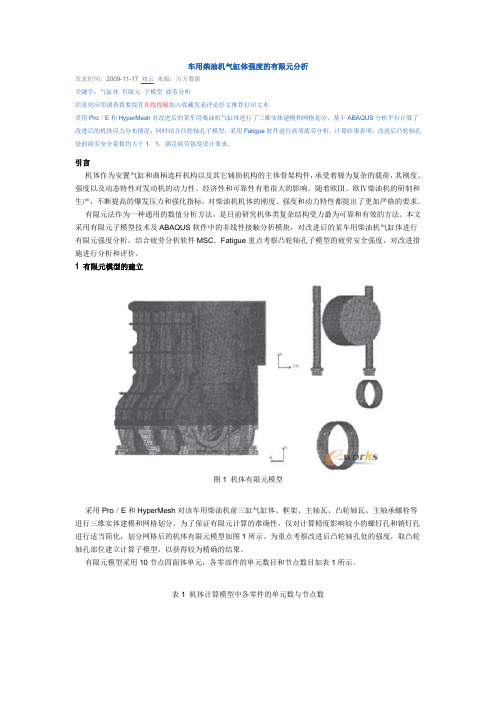
车用柴油机气缸体强度的有限元分析发表时间：2009-11-17 刘云来源：万方数据关键字：气缸体有限元子模型疲劳分析信息化应用调查我要找茬在线投稿加入收藏发表评论好文推荐打印文本采用Pro／E和HyperMesh对改进后的某车用柴油机气缸体进行了三维实体建模和网格划分，基于ABAQUS分析平台计算了改进后的机体应力分布情况；同时结合凸轮轴孔子模型，采用Fatigue软件进行高周疲劳分析。

计算结果表明：改进后凸轮轴孔处的疲劳安全系数均大于1．1，满足疲劳强度设计要求。

引言机体作为安置气缸和曲柄连杆机构以及其它辅助机构的主体骨架构件，承受着极为复杂的载荷，其刚度、强度以及动态特性对发动机的动力性、经济性和可靠性有着很大的影响。

随着欧Ⅲ、欧Ⅳ柴油机的研制和生产，不断提高的爆发压力和强化指标，对柴油机机体的刚度、强度和动力特性都提出了更加严格的要求。

有限元法作为一种通用的数值分析方法，是目前研究机体类复杂结构受力最为可靠和有效的方法。

本文采用有限元子模型技术及ABAQUS软件中的非线性接触分析模块，对改进后的某车用柴油机气缸体进行有限元强度分析，结合疲劳分析软件MSC．Fatigue重点考察凸轮轴孔子模型的疲劳安全强度，对改进措施进行分析和评价。

1 有限元模型的建立图1 机体有限元模型采用Pro／E和HyperMesh对该车用柴油机前三缸气缸体、框架、主轴瓦、凸轮轴瓦、主轴承螺栓等进行三维实体建模和网格划分。

为了保证有限元计算的准确性，仅对计算精度影响较小的螺钉孔和销钉孔进行适当简化，划分网格后的机体有限元模型如图1所示。

为重点考察改进后凸轮轴孔处的强度，取凸轮轴孔部位建立计算子模型，以获得较为精确的结果。

有限元模型采用10节点四面体单元，各零部件的单元数目和节点数目如表1所示。

表1 机体计算模型中各零件的单元数与节点数2 载荷与边界条件由于重点考察主轴承力对机体尤其是凸轮轴孔的影响，故对机体顶面节点进行约束。

基于hypermesh的发动机零部件网格划分

能．总结出针对不同发动机零部件的网格划分方法有利于提高有限元分析的效率与准确性，还可帮助从事相关有限元分析的人员快速掌握发动机主要零部件的网格划分技巧。参考文献
【１】谭继锦，张代胜．汽车结构有限元分析【Ｍ】．北京：清华大学出
版社，２００９：１５６．
【２】杜平安，于亚婷等．有限元法原理、建模及运用［Ｍ】．北京：国
各体块进行网格划分．也可用ｍｕｌｔｉｓｏｌｉｄｓ功能对各体块进行自动网格划分。连杆和四分之一活塞模型的网格划分如图９和图１０所示。
连杆和活塞在结构上并不是由一些拉伸、旋转和扫掠体简单地组合在一起构成的，而且还有许多
一一
万方数据
３０
内燃机与配件
２０１４年第ｌ期
４气缸盖和机体的网格划分
气缸盖和机体的结构非常复杂，要对它们进行六面体网格划分需要耗费大量的人力和时间。一般情况下会选择对气缸盖和机体进行四面体网格划分，而非六面体。在进行大变形和碰撞分析时更是如此。在ｈｙｐｅｒｍｅｓｈ软件中划分四面体网格一般有两种方式。一是先用２Ｄ面板下的ａｕｔｏｍｅｓｈ子面板对气缸盖和机体的表面进行２Ｄ网格划分。并对表面网格进行质量控制．然后进入到３Ｄ面板下的ｔｅ．ｔｒａｍｅｓｈ子面板中的Ｔｅｔｒａｍｅｓｈ功能按钮．软件会根据已有的２Ｄ网格自动划分３Ｄ四面体网格。第二种方式是进入到３Ｄ面板下的ｔｅｔｒａｍｅｓｈ子面板中的
ｓｏｌｉｄ
凸轮轴和曲轴都是由多个拉伸体组成的，而且
都是由一个相同的结构，通过旋转一定的角度组合在一起的。如对于凸轮轴而言这个重复的相同结构通常是由一或两个凸轮和一个轴颈组成的。对凸轮轴和曲轴的六面体网格划分应先将重复的相同结构逐个切分，然后再将其分割成一个个简单的拉伸体。凸轮轴重复结构的分割如图４所示。之后对拉伸体的拉伸起始面进行四边形网格划分，最后通过这些２Ｄ网格生成３Ｄ六面体网格。凸轮轴和曲轴重复结构的网格划分如图５和图６所示。以上操作所用的ｈｙｐｅｒｍｅｓｈ中的功能与气门网格划分相同。

轿车发动机盖抗凹性分析

Altair 2009 HyperWorks 技术大会论文集轿车发动机盖抗凹性分析肖介平张立玲郁向东叶子青北京汽车研究总院 CAE 技术部门-1-Altair 2009 HyperWorks 技术大会论文集轿车发动机盖抗凹性分析 Outer Panel Denting Analysis of Car Hood肖介平张立玲郁向东叶子青（北京汽车研究总院 CAE 技术部门北京 100021）摘要:轿车外覆盖件的抗凹性直接影响整车的外观品质。

本文借助于 HyperMesh 前处理平台建立了某轿车发动机盖的有限元模型，采用 ABAQUS 求解器对发动机盖的指压和罐压两种工况进行了数值模拟分析，给出了相关评价标准，对轿车发动机盖的抗凹性设计具有一定的指导意义。

关键词: HyperWorks,HyperMesh，发动机盖，抗凹性，指压，罐压 Abstract: The out panel's dent resistance ability could directly affect the appearance quality of wholecar. The FEM model of a car hood was built using HyperMesh, and hood’s dent resistance including the dimpling and oil-canning denting was analyzed using ABAQUS solver. The analysis method and evaluation criterions in denting simulation could have some guiding significance on the design of the car hood denting.Key words: HyperWorks, Hood, Denting, Dimpling, Oil-canning1 概述发动机盖抗凹性分析是评价其在使用过程中，受到如手指触摸按压，罐状物体挤压等载荷工况下外板薄弱区域抵抗凹陷挠曲的能力，即考察载荷作用下的最大变形情况和局部区域在卸载后的永久变形情况。

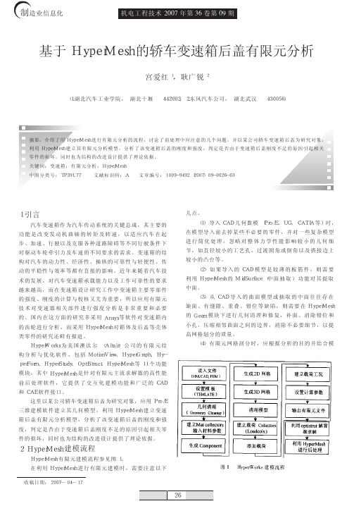
基于HyperMesh的轿车变速箱后盖有限元分析

的有限元分析软件，进入国
图６拉丝拉力作用在拉丝支架上变速箱后盖的变形图、应力分布图
内仅有几年的时间，因此需要在进一步的工程应用中不
断总结和积累经验。
参考文献：
［１］陈家瑞．汽车构造［Ｍ］．
北京：机械工业出版社，
２００２．
［２］刘惟信．汽车设计［Ｍ］．
这里以某公司轿车变速箱后盖为研究对象，应用Ｐｒｏ／Ｅ三维建模软件建立其几何模型，利用ＨｙｐｅｒＭｅｓｈ建立变速箱后盖有限元分析模型，分析了该变速箱后盖的刚度和强度，判定是否由于变速箱后盖刚度不足的原因引起相关零件的损坏，同时也为结构的改进设计提供了理论依据。
（６）施加载荷和边界条件是有限元分析最为关键的一环，它对分析结果有着决定性的影响，对结构分析来说，要让自己的约束和载荷尽量与实际情况相符，这样我们得到的分析结果才能有意义，这一步需要我们在平时的工作中不断的摸索和积累经验来实现。
３变速箱后盖有限元模型的建立
（１）零件分析 ①结构特征：变速箱后盖为一个较为复杂的盘式空间结构，主要结构特征为用于固定的三个安装孔、与发电机支架的七个连接孔、中心处的一个轴承孔和十四个加强筋以及一些倒角等附属结构。 ②受力情况：在其与发电机支架的七个连接孔中心处施加１７８Ｎ·ｍ扭矩，同时在其中两个孔中心处施加４２０Ｎ的离合器拉丝拉力，另外，还考虑了发电机的自重载荷２３５．２Ｎ。 ③材料特性：镁合金，泊松比 μ＝０．２８，弹性模量Ｅ＝４５ＧＰａ，密度 ρ＝１．７×１０３ｋｇ／ｍ３。 ④分析方案：分析考虑了将离合器拉丝拉力分别施加在孔中心和拉丝支架上、不加拉丝拉力三种计算方案。运用Ｐｒｏ／Ｅ建立变速箱后盖几何模型如图２所示，并以ＩＧＥＳ中性文件格式输出。

Abaqus 在汽车发动机罩铰链强度分析中的应用,长城汽车股份有限公司技术中心

论文所属行业:汽车Abaqus在汽车发动机罩铰链强度分析中的应用梁艮文，盛守增，王俊长城汽车股份有限公司技术中心，河北省汽车工程技术研究中心，河北省保定市071000摘要：文章采用Abaqus软件非常强大的非线性有限元知识对汽车发动机罩铰链进行强度分析，分析结果为发动机罩铰链结构设计提供参考。

关键词：发动机罩；铰链；强度Abaqus Application To Strength AnalysisFor Automotive Bonnet HingeLIANG Genwen, SHENG Shouzeng, WANG JunR&D Center of Great Wall Motor Company, The Automobile Engineering Technology & Research Center ofHebei Province, Bao Ding, 071000, hebei, chinaAbstract: The article is strength analysis for automotive bonnet hinge introducing Abaqus software powerful nonlinearity finity knowledge, the analysis results provide a reference for the bonnet hinge design. Key words: bonnet; hinge; strength0 引言随着人民生活水平的不断提高，汽车作为一种方便、舒适的交通工具得到越来越多的消费者青睐。

由于交通事故的频繁发生，消费者在购车过程中更加重视汽车的安全性及可靠性。

发动机罩的主要作用是方便机舱内各零部件的维修保养，保护机舱内各零部件，隔离噪声，保护行人。

发动机罩铰链用来固定和旋转发动机罩，它的强度对发动机罩发挥其作用有着非常重要的意义。

交通运输——基于Abaqus的发动机缸体缸盖密封性能研究

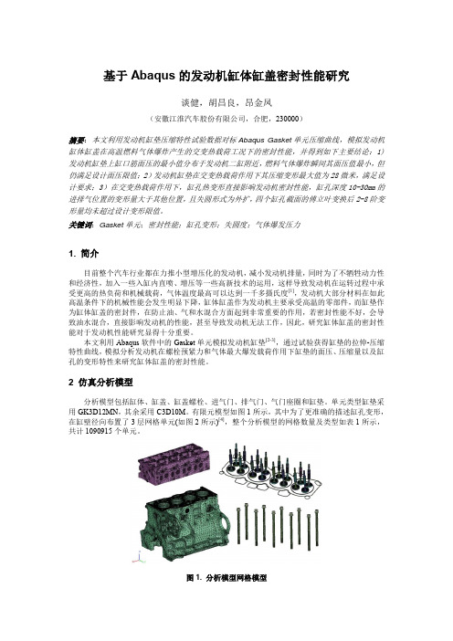
基于Abaqus的发动机缸体缸盖密封性能研究谈健，胡昌良，昂金凤（安徽江淮汽车股份有限公司，合肥，230000）摘要：本文利用发动机缸垫压缩特性试验数据对标Abaqus Gasket单元压缩曲线，模拟发动机缸体缸盖在高温燃料气体爆炸产生的交变热载荷工况下的密封性能，并得到如下主要结论：1)发动机缸垫上缸口筋面压的最小值分布于发动机二缸附近，燃料气体爆炸瞬间其面压值最小，但仍满足设计面压限值；2）发动机缸垫在交变热载荷作用下其压缩变形最大值为28微米，满足设计要求；3）在交变热载荷作用下，缸孔热变形直接影响发动机密封性能，缸孔深度10-30mm的进排气位置的变形量大于其他位置，且失圆形式为外扩，四个缸孔截面的傅立叶变换后2-8阶变形量均未超过设计变形限值。

关键词：Gasket单元；密封性能；缸孔变形；失圆度；气体爆发压力1. 简介目前整个汽车行业都在力推小型增压化的发动机，减小发动机排量，同时为了不牺牲动力性和经济性，加入一些入缸内直喷、增压等一些高新技术的运用，这样导致发动机在运转过程中承受更高的热负荷和机械载荷，气体温度最高可以达到一千多摄氏度[1]，发动机大部分材料在如此高温条件下的机械性能会发生明显下降，缸体缸盖作为发动机主要承受高温的零部件，而缸垫作为缸体缸盖的密封件，在防止油、气和水混合方面起到非常重要的作用，若密封性能不好，会导致油水混合，直接影响发动机的性能，甚至导致发动机无法工作，因此，研究缸体缸盖的密封性能对于发动机性能研究显得十分重要。

本文利用Abaqus软件中的Gasket单元模拟发动机缸垫[2-3]，通过试验获得缸垫的拉伸-压缩特性曲线，模拟分析发动机在螺栓预紧力和气体最大爆发载荷作用下缸垫的面压、压缩量以及缸孔的变形特性来研究缸体缸盖的密封性能。

2 仿真分析模型分析模型包括缸体、缸盖、缸盖螺栓、进气门、排气门、气门座圈和缸垫。

单元类型缸垫采用GK3D12MN，其余采用C3D10M。

1、下载文档前请自行甄别文档内容的完整性，平台不提供额外的编辑、内容补充、找答案等附加服务。
2、"仅部分预览"的文档,不可在线预览部分如存在完整性等问题,可反馈申请退款(可完整预览的文档不适用该条件!)。
3、如文档侵犯您的权益，请联系客服反馈,我们会尽快为您处理(人工客服工作时间：9:00-18:30)。

581
值与试验结果相对误差基本在 5% 以下，符合工程实际要求的精度。这表明气缸盖的有限元模型能较好地反应气缸盖的动态特性。
3 结语
采用 Hypermesh 软件对整个气缸盖直接划分网
格，成功地建立了气缸盖的有限元模型，解决了复杂的零部件建模难的问题。在 Abaqus 中对模型进行模态分析计算，得到了所需要的模态参数。
Hypermesh 是一个高效的有限元前后处理器，能够建立各种复杂模型的有限元和有限差分模型，与多种 CAD 和 CAE 软件有良好的接口并具有高效的网格划分功能［7］。Abaqus 则是一款功能强大的有限元软件，可以分析复杂的固体力学和结构力学系统，模拟庞大复杂的模型，处理高度非线性问题［8］。通过这两款软件的结合使用，便可完成极其复杂的零部件有限元分析。
气缸盖三维模型( 见图 1) 倒角、小孔非常多。
对于这种多孔多曲面部件的有限元建模一直是一
个难点。文中采用 Hypermesh 软件作为网格划分工
具，在保证质量的前提下，能够快速完成整个气缸
盖的网格划分工作。
图 1 气缸盖三维模型
Fig． 1 Three-dimensional model of cylinder head
Abstract: With the combination of the two CAE software Hypermesh and Abaqus，the universal difficulty of modeling complicated finite elements is solved． The cylinder head of a diesel engine is successfully modeled． Modal analysis is carried out and the first six natural frequencies and mode shapes were extracted． By examining the data of modal analysis，the deviations are within 5% ，which explains rather high precision of the finite model and the accuracy of finite elements analysis． The present work lays the foundation for optimization design and dynamic analysis of cylinder head． Key words: cylinder head，modal analysis，experimental modal analysis
表 1 气缸盖固有频率 Tab． 1 Natural frequencies of cylinder head
模态阶次
1 2 3 4 5 6
计算值 1 158 1 440 1 885 2 467 2 775 3 030
频率 /Hz 实验值 1 110 1 370 1 800 2 370 2 690 2 920
半来进行分析计算［5］; 梁莎莉等人为保证气缸盖计算分析的准确性，建立计算模型时，对其主要结构尺寸不作简化，对复杂水腔和气道均采用实际铸造砂芯尺寸建模，以保证计算结果的准确性［6］。早期， Hell J S 等对气缸盖进行有限元计算时对其复杂的结构进行过分简化，把复杂的水腔简化成简单的箱形结构，弯曲的气道则用简单的圆柱、圆锥等几何元素来代替。
图 3 气缸盖前 6 阶振型 Fig． 3 First six mode shapes of cylinder head
1． 4 模态试验为了验证模型的准确性，对结构进行模态
测试。
1) 试验仪器 B＆K 560C 型 PULSE 振动与声学分析系统。 2) 试验方法利用锤击模态试验法，设置测试频率范围为 0 ～ 3 200 Hz，由传递函数获取结构的固有频率等参数。测试系统原理图如图 4 所示。为避免遗漏结构的模态，分别在气缸盖的不同面上布置传感器，并采用多点锤击，以避免由于锤击点在节点上带来的不准确性［9］。文中试验将传感器分别放在气缸盖的两个不同面上，每次测试 9 个点，其中每个点敲击 10 次，取平均值。然后，将传感器在不同位置时测出的值进行对比，以验证测试结果是否准确。气缸盖的悬挂采用柔性绳，悬挂位置和锤击点位置分布如图 5 所示。
贺信菊1，卜安珍2，夏兴兰2，钱怡1*
( 1. 江南大学机械工程学院，江苏无锡 214122; 2. 无锡油泵油嘴研究所，江苏无锡 214063)
摘要: 采用 CAE 软件 Hypermesh 与 Abaqus 相结合，解决了复杂结构有限元建模难的普遍难题。建立了某柴油发动机气缸盖的有限元分析模型，并进行模态分析，提取了前 6 阶固有频率及振型。通过试验模态分析数据检验，误差基本在 5% 以内，说明有限元模型具有较高的精度，同时证明有限元分析的准确性，为气缸盖的优化设计和动力学分析打下了基础。关键词: 气缸盖; 模态分析; 试验模态分析中图分类号: TH 113． 2; TH 113． 1 文献标识码: A 文章编号: 1671 － 7147( 2011) 05 － 0578 － 04
采用 Hypermesh 快速划分复杂零件四面体网 105 MPa，泊松比为 0． 27; 模型总节点数为 43 593，单
格时的基本思想是先生成面网格，然后由面网格生元数为 145 747。
成体网格。首先清理三维模型，删除一些影响网格
质量但又对分析计算影响不大的小孔小面等。一些
1 模态分析原理与气缸盖模型分析
1． 1 模态分析原理模态是机械结构的固有振动特性，每一个模态
具有特定的固有频率、阻尼比和模态振型。对于一个多自由度系统，其振动方程［3］为
［M］{ X¨ } + ［C］{ ·X} + ［K］{ X} = { F( t) } ( 1)
综上可见，在少量简化的前提下，对整个气缸盖直接建立有限元模型是比较困难的。因此文中利用 Hypermesh 和 Abaqus 两款软件结合完成气缸盖的模态分析。首先在 Hypermesh 完成气缸盖整体网
收稿日期: 2011 － 08 － 20; 修订日期: 2011 － 09 － 07。作者简介: 贺信菊( 1985—) ，女，重庆人，机械设计专业硕士研究生。 * 通信作者: 钱怡( 1962—) ，女，江苏无锡人，副教授，硕士生导师。主要从事机械及包装结构的动、静态性能等
图 5 测试现场 Fig． 5 Test site
图 4 试验系统原理 Fig． 4 Test system schematic
2 有限元结果与试验结果比较
表 1 列出了通过有限元法和试验模态分析所得的气缸盖的前 6 阶固有频率，传递函数如图 6 所示。
读取图中各曲线峰值重叠较多处的频率即为该结构的固有频率。
1． 3 气缸盖自由模态分析结果图 3 为采用 ABAQUS 分析的气缸盖的模态结
果。从振型图可以看出气缸盖在不同频率下的主振
580
江南大学学报 ( 自然科学版)
第 10 卷
型: 第 1 阶振型为平面弯曲; 第 2 阶振型则以扭转为主; 第 3 阶振型为缸盖整体绕 Z 轴的弯曲变形。
通过试验验证，表明该方法不仅建模便捷，且具有较高的精度，对复杂结构的有限元建模、分析具有指导意义。
误差率 /% 4． 3 5． 1 4． 7 3． 7 3． 1 3． 8
从表 1 可以看出，计算值都略高于实验值，这是因为在前处理时删除了部分小孔和倒角，导致模型刚度有少许提高。尽管如此，气缸盖模态分析计算
第5 期
贺信菊等: 基于 Hypermesh 和 Abaqus 的气缸盖动态特性分析
( 2)
式中: ω 为自由振动固有频率; ［M］，［K］分别为结
构质量、刚度矩阵。
特征方程为 | ［K］－ ω2［M］| = 0
展开行列式，得到关于 ω2 的 n 次多项式的特征值，
即为离散模型的固有频率，将特征值带入式( 2) 就
可得出特征向量，从而获得给定频率下的振型。
1． 2 气缸盖有限元模型的建立
研究。Email: yi － qian@ jiangnan． edu． cn
第5 期
贺信菊等: 基于 Hypermesh 和 Abaqus 的气缸盖动态特性分析
579
格的划分，然后导入 Abaqus 中完成模态分析计算，并通过模态试验来验证计算结果，为气缸盖的设计和优化人员提供理论依据以及建模方法的参考。
图 2 缸盖有限元网格
生成体网格。当个别面网格不能生成体网格时，需重新调整，直至能生成体网格为止。
图 2 为气缸盖的四面体单元有限元模型，其材料为 HT250，密度为 7 280 kg / m3 ，杨氏模量为 1． 3 ×
Fig． 2 Finite element mesh of cylinder head
第 10 卷第 5 期 2011 年 10 月
江南大学学报( 自然科学版) Journal of Jiangnan University( Natural Science Edition)
Vol． 10 No． 5 Oct． 2011