Hypermesh和Abaqus的接口分析实例
abaqus与hypermesh接口教程
Consider a 96 in. x 12 in. cantilever beam as shown in the above figure. The beam is loaded at the right end by a force P = 40000 lb. The beam is isotropic with Young’s modulus E = 3x10⁷psi and Poisson’s ratio ν= 0.3. Using Hypermesh and ABAQUS, perform the analysis outlined below. Start out by creating a relatively coarse mesh of 4-node quadrilateral elements (try a mesh of rectangular elements with 6 divisions in the x direction and 2 divisions in the y direction). Apply the appropriate boundary conditions, and run the problem assuming plane stress.Instructions for Lab#2Using Hypermesh and ABAQUS for the analysis of a beam in bending.Figure 1. Main Window in Hypermesh. Circled is the command toolbar that allows the user to access sub menus.Getting Acquainted1) Fire up Hypermesh from the menu controls.2) Familiarize yourself with the command toolbar to your right. By clicking next to eachtitle as circled above, you will be brought to several sub-menus where you may perform a variety of tasks. Click on each and analyze each sub-menu.3) Identify commands that appear self-explanatory, such as file, automesh, nodes,lines, ect....4) Notice that the file command exists in every toolbar.5) Click on the file command. This is where you name the hypermesh files you wouldlike to save using a *.hm extension. Also, this is where importing and exporting occurs.6) Also notice the template command. This is where the solvers are invoked.Hypermesh has the capability of exporting mesh information for a variety of solvers.Keep in mind, Hypermesh is purely a mesh generator and the mesh information must be translated into the format of the desired solver to be used, therefore picking the correct solver from the template is a necessary step before continuing with any other stepsGeometryIn this exercise we will generate the geometry of a beam to be deformed by applying a tip point load and by fixing one end. After completion of the geometry generation, a 3-dimensional mesh of the beam will be created and a stress analysis on the beam will be performed.1) Like all mesh generators, in order to create a mesh, some geometry must exist.Generally nodes are required from which lines are created. Surfaces must be created from a set of lines that form a closed loop. It is those surfaces that will be meshed.2) Click on the “Geom” icon to your right and notice the various menus. In particular,notice the “nodes” icon. Clicking on that will allow to create several nodes in a variety of modes. For example, by co-ordinates (most popular one), on lines, ect..3) Once the nodes exist, one can create lines from those nodes by clicking on the“line” button. Note the options available for the different type of lines that can be created. Go ahead and create lines from the existing nodes.4) With the lines created, surfaces can be generated by clicking on the “surface edit”button and by selecting the filler surface option. Create a surface using all existing lines.5) At this point the geometry has been created and mesh generation should be thenext step.Mesh generationIn this phase of the exercise the geometry created above will be meshed. The first step will be to mesh the two-dimensional surface with 2-D elements. Two meshes will be generated, a biased mesh and regular mesh. Samples can be seen in the figures below. When that is done, the two meshes will be extruded to create the three-dimensional brick element meshes.Figure 2. A simple quad mesh with no biasing.Figure 3. A biased quad mesh focused toward one end.Creating a 2-D mesh.1) With all surfaces created, it is time to mesh.2) Prior to creating elements, the concept of “collectors” must be reviewed.Hypermesh has the ability to store groups of elements under different names called collectors. In this manner, it is possible to modify parts of a mesh on a group basis.We will practice using these collectors to store the two meshes that will be generated for the same part. In one collector we will store the elements for the mesh in figure 2 and in another collector we will store the mesh for figure 3. To create collectors, click on the “collectors” button and create the two collectors using two different names and two different colors.3) You can toggle between the two collectors by using the “global button” in the righthand bottom corner and selecting the collector you wish to work in. It is important that you know which collector is being used as default and changing it will be necessary as the meshing progresses. Further you may display the desired collectors by using the “display” command in the bottom right corner and by clicking and un-clicking on each collector that is available. With that done we may proceed to create the two meshes.4) Make sure you know which collector is currently set to default. To begin meshing,click on the 2D toolbar to your right.5) There are a variety of options available. We will use the automesh option.6) By clicking on automesh, several parameters are required as well as the necessityto select the surfaces one wants to mesh.7) Select the surface by clicking on each and supply a rough idea of the element sizeand element type you would like to use. Also make sure you are in the interactive mode.8) Once that is done, clicking the mesh button will generate a tentative idea of howyour mesh will look along the geometry borders. You may enhance your mesh by improving on the coarseness, adding bias, ect... By clicking on the number of divisions for each line you may increase that value using the left button or decrease that value using the right button. Similar things can be done if one wants to change the bias or other parameters.9) With that done, clicking on the mesh button will create the mesh. Accept the meshby clicking return or reject it by clicking reject.10) T he above steps must be repeated to create a biased mesh toward the fixedlocation. To do that repeat steps 3-8, but ensuring yourself that you are in the appropriate collector. Also, when the tentative divisions on the border of your surface appear, you can add bias by clicking on the bias button and giving positive or negative bias values.Note: Your part may consist of several surfaces and you may mesh them all at once or separately. You may also allocate each meshed portion to different collectors, so as to be able to have control over your model based on the different portions meshed.Creating a 3-D mesh.1) The next step involves extruding the mesh from its 2-D version, thus creating a 3-Dmesh.2) The first step is two create two additional collectors into which the two 3-D mesheswill be saved.3) With that done, click on the “3D” button and click on the drag button.4) The drag button allows the user to drag a set of 2-dimensional elements into 3-dimensional elements so long that a drag direction and distance are supplied, as well as the intended number of divisions to be created on the way.5) Select the elements to be dragged by component and define a drag direction anddistance. Supply the intended number of divisions. With that done, click on the drag button. Your 3-dimensional mesh will be created within the chosen collector.6) Do the same for the second 2-dimensional mesh and ensure that it is put in theappropriate collector.7) With that done, it will be necessary to delete the unnecessary 2-dimensionalmeshes. To do so press the F2 key and delete elements by component and select the two components to be deleted. Click on “delete” to approve deletion of the two selected components.Boundary conditionsOnce the mesh has been created, it is necessary to create the required boundary conditions. Boundary conditions can be created within Hypermesh for use in ABAQUS, however the complexity of the steps within Hypermesh, outweighs the ease of typing in boundary conditions within the ABAQUS file, provided that the appropriate node sets and element sets are available. This is what will be done in the next steps.1) We need two sets. A node sets for those nodes that will be fixed and a node set forthose nodes onto which the load will be applied.2) To do so, click on the BCs menu. There you will create entity sets. Entity sets issimply a manner to groups nodes or elements under one common name. In ABAQUS, boundary conditions can be applied to those sets.3) Click on entity sets and create a node set called “fixed”. Select the nodes on the leftend of the beam by using the window select. When done click on create. If the set is created, click on RESET.4) Change the name to “load” and select the nodes onto which the load will be appliedand click on create.5) This will be it!With the mesh completed you may now export your file using the ABAQUS template and saving the file under a *.inp extension. You can do this by clicking on file and then selecting the export command. MAKE SURE YOU ARE USING THE “ABAQUS STANDARD” TEMPLATE. Be careful here!NOTE: Remember you have two meshes on top of each other. Before you export each mesh as *.inp file, you must create to separate Hypermesh files. In each file save only the mesh you desire. This is done by deleting the unwanted mesh and saving under a different name. Deleting elements or nodes is accomplished using the F2 command. It is also a good idea to go ahead and renumber your mesh when you are ready to finalize it. Renumbering is accomplished by clicking on the tools icon and then clicking on the renumber button. Do this for each mesh. Now we are ready for ABAQUS.IN ABAQUSThe general ABAQUS file follows your typical format for any FEA solver. It contains nodal information and connectivity as well as element type information. At the end are the boundary conditions and the solution procedure. This can be observed below.Open the *.inp file that was created. It should look as follows:**** ABAQUS Input Deck Generated by HyperMesh Version3.0**** Template: ABAQUS/STANDARD***** THIS IS THE NODAL INFORMATION*NODE1, 0.0 , 2.221825 , -7.778174: : :: : :: : :9843, 6.7033386359838, 3.648821000031 , 0.0539689803571*** THIS IS THE ELEMENT INFORMATION. C3D8= 8 noded brick element.*ELEMENT,TYPE=C3D8,ELSET= threeD1, 1858, 1857, 1878, 1879, ………….: : :: : :: : :8470, 478, 522, 9807, 9774, ……….** SECTION DEFINITION: assign material and thickness if necessary for shells.*SOLID SECTION, ELSET= threeD, MATERIAL= ALUMINUM*** HERE ARE THE ENTITY SETS TO BE USED FOR THE B.C.’s*NSET, NSET= fixed1, 2, 3, 4, 5, 6, 7, 8,9, 10, 11, 12, 13, 14, 15, 16,*NSET, NSET= load448, 449, 450, 451, 452, 453, 454, 455,**** MATERIAL PROPERTIES*MATERIAL, NAME= MAT1*ELASTIC, TYPE = ISOTROPIC10000000.0,0.22,0.0********THIS IS WHAT YOU ADD MANUALLY LOAD STEP INFORMATION, BOUNDARY CONDITION INFORMATION, AND OUTPUT INFORMATION.******STEP*STATIC --- TYPE OF ANALYSYS*CLOAD --- TYPE OF LOADload,1,-1.0*BOUNDARY --- TYPE OF DISPLACEMENT BCfixed,1,3,0.0*EL FILE --- ELEMENT OUTPUT TO BE VIEWED IN HYPERMESHSINV*NODE FILE --- NODAL OUTPUT TO BE VIEWED IN HYPERMESHU*EL PRINT, ELSET=threeD --- ELEMENT OUTPUT TO BE LISTED IN DATA FILES11,S22,S33,S12,S13,S23E11,E22,E33,E12,E13,E23*NODE PRINT, NSET=fixed --- NODAL OUTPUT TO BE LISTED IN DATA FILEU,RF*END STEPWith this in mind, you should modify your file to include necessary analysis information and boundary conditions. When that is done, you can run your two ABAQUS filesVIEWING THE RESULTS IN HYPERMESH.Once the ABAQUS run is complete, you need to convert the *.fil into a hypermesh *.res file. Do this by using the hmabaqus command within your unix template. Now open Hypermesh.1) Retrieve one of the models and click on the global button.2) You will see a path for the results file. Enter the filename assigned above.3) Exit this menu and click on the POST icon and view your results by using thecontour button.Some contour plots of a beam in bending. You may create displacement contours, stress contours, ect…Figure 4. The displacement contour plot for a beam in bending.Figure 5. Von-Mises Stress Contour for a beam in bending.General Tips:1) When meshing a model in separate portions it is necessary to create a collector foreach portion and making sure one has selected the correct collector before meshing a surface so that those elements created are fed into the desired collector2) Also, one must always check for duplicate elements or nodes. This can be donewith appropriate commands in the tools toolbar available at your right. We will explore these commands in class.。
hypermesh与Abaqus联合仿真经典教程ppt课件

.
13
8, 设置载荷步
A,选择load steps 命令,设置第一个载荷步
B,载荷步的名字应该清楚的说明加载的情况 勾选载荷步包含的载荷(loadcols)及输出设置(outputlocks),点击update
C ,点击edit ,进入载荷步参数设置页面
.
14
8, 设置载荷步
C-1,step parameter 选择
注意:刚性网格的单元类型要更新成R3D3、R3D4,普通单元类型是S3、S4。 命令是2D/elem types
.
4
4, 焊点,单元类型是1D/rigid/Beam
选择多点方式 连接焊点位置上下各一个单元的点,连接完成后,显示BEAM 单元类型
.
5
4, 焊点,一维单元类型转换1D/config edit
初始步长
最小步长 最大步长
C-3,Load_OP 选择
Load_OP用来设置是否需要保留上一步 的边界条件(Boundary)或者是载荷(集 中载荷Cload 、面载荷Dload)
OP=MOD,表示保留上一步设置 OP=NEW,表示不保留上一步设置
程序默认值是OP=MOD
.
15
8, 设置载荷步
D,第二个载荷步的设置
现在模型里面用的是单点连接,也行,但是单元类型spring不对,需要转换成Beam。 选择config edit命令
A,选择要转换的单元
B,选择新单.元类型rigid
C,转换 6
5, 边界条件及载荷设置
A, 建立约束loadcol
B, 设置约束
C, 建立加载 loadcol ,加载力或者通过约束加强迫位移
E_1a
选择单元,显示法向
精编hypermesh与Abaqus联合仿真经典教程

6, 接触对的设置
F, 设置接触对
直接选择设好的接触属性和接触面
下面这些接触参数,常用的有adjust、smooth、tie、smallsliding. 如果对这些参数没有理解,可以先不选。
7, 输出设置
A,选择output block 命令
B,在file文件中输出点的位移及约束反力, 单元的应力应变 (U ,RF,SINV ,PE),特殊结果输出参数,参考Abaqus手册。
8, 设置载荷步
A,选择load steps 命令,设置第一个载荷步
B,载荷步的名字应该清楚的说明加载的情况 勾选载荷步包含的载荷(loadcols)及输出设置(outputlocks),点击update
6, 接触对的设置
E, 调整需要添加接触的单元法向相对, 然后添加接触单元
E_1 检查并调整接触网格的单元法向
E_1a
选择单元,显示法向
E_1b
选择法向一致的参考单元
E_1c
调整法向,法向指向接触面
6, 接触对的设置
E, 调整需要添加接触的单元法向相对, 然后添加接触单元 E_2 添加接触单元到主从接触面
2, 材料建立
A,选ity,输入材料密度。注意:单位制(吨t,毫米mm,牛N,兆帕MPa,秒S)
C,勾选Elastic,输入材料线性属性,弹性模量E,及泊松比NU
试验应力应变曲线值需要 转换成材料的真实应力-塑 性应变曲线。 转换公式参考相关资料。 下面的文件包含转换模板。
OP=MOD,表示保留上一步设置 OP=NEW,表示不保留上一步设置
程序默认值是OP=MOD
8, 设置载荷步
D,第二个载荷步的设置
hypermesh与abaqus接口连接经典实例
hypermesh与abaqus接口连接经典实例模型中考虑了材料、几何的非线性、接触和Tie连接,所有设置都在HM中完成,输出inp文件后可以直接在Abaqus中计算。
尤其注意在HM6.0中利用宏菜单中的Abaqus Contact Manager来定义接触、Tie连接等问题。
欢迎大家批评指正。
同时该算例仅仅是一个step的,如果哪位能将其扩展到多个step,还会给以积分奖励。
再加一些步骤说明:问题描述:如下图所示模型,模型整体分为三部分,黄色的tube、深蓝色的holder和浅蓝色的welded_part。
其中tube和holder部分属于接触,而holder和welded_part两部分的连接属于焊接,这里采用Abaqus中的Tie连接方式。
最后固定welded_part的一端,而在tube的一端施加一个扭矩,为了保证不发生刚体位移,在tube的另一端施加一个止推的约束。
定义ABAQUS模板:在Geom页面上选择user prof…,从弹出菜单中选择ABAQUS,然后选择Standard 3D。
为保证问题具有一般性,对上述模型划分的网格在连接的部分均保证网格不对齐,在宽度和圆周上均采用了不同的网格密度。
单元类型的设置:因为涉及接触问题,所以模型中的实体单元均采用Abaqus中的C3D8R减缩积分单元,单元类型的选择请参考Abaqus使用手册。
在HyperMesh中改变单元类型的步骤如下:1.在1D、2D和3D的任何一个页面中点击elem types。
2.选择2d&3d子面板,根据单元的结构选择单元类型,在这个例子中点击hex8,从弹出菜单中选择C3D8R。
3.选中要更新单元类型的单元,这里选择by collector(选择所有三个comps)。
4.点击update。
5.如果需要察看现有任意一个单元的类型,在永久菜单上点击card,将操作对象设为elem,选择单元后点击edit。
就可以看到单元的类型。
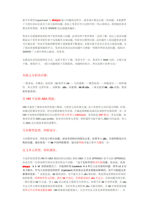
ABAQUS与Hypermesh接口流程原创
ABAQUS与Hypermesh接口流程本文分两种情况。
第一种:在HM中对几何模型全部建好网格,导入ABAQUS中分析。
第二种:在ABAQUS中已有的计算模型根底上,再导入网格部件重新整合进展分析。
第一种情况:1.在ABAQUS中建好几何模型〔如图1所示〕,如果是用其他造型软件建的模型也要先导入ABAQUS,然后对模型进展装配,为的是确定全局坐标系,在后续的操作中全局坐标系不要再改变。
图12.导出ACIS SAT文件,后缀名为.sat,如图2和图3所示。
图2 图33.翻开HM,注意设定user profiles为ABAQUS,如图4所示。
图44.导入几何模型,如图5所示。
图55.处理几何模型,例如:布尔运算,消除硬点等。
设置网格类型,画网格,将模型划分成数个网格部件。
如图6所示,几何模型被划分成了两个网格部件,根据仿真计算的需要也可对两个小块布尔求和,划分成一个网格部件。
一个网格部件就是一个网格节点相连的网格体,只含有网格节点、单元、集合信息。
图66.导出网格,文件格式为.inp,如图7所示。
图77.导入ABAQUS〔如图8,图9和图10所示〕,继续设置其他前处理。
图8 图9图10第二种情况:在已有的分析根底上添加网格部件1.首先,将需要划分网格的几何模型导入ABAQUS,进展装配,如图11所示。
该步骤为的是确定几何模型的全局坐标,方便后续的导入。
图112.导出该几何模型的.sat文件,导入HM划分网格,如图12所示。
图123.划分网格后,导出inp文件。
用记事本翻开导出的inp文件和原有分析模型的inp文件,将导出的inp文件中的一段网格单元信息粘贴进原分析模型的inp文件中,另存为一个inp文件,重新翻开该文件进展后续的处理。
说明:关于inp文件参考"ABAQUS有限元分析常见问题解答"第13章。
两个inp文件的融合方法,原已有计算模型的inp文件如下〔粗体显示的为需要添加的代码的格式〕:*Heading** Job name: 111 Model name: e*1** Generated by: Abaqus/CAE 6.9-1*Preprint, echo=NO, model=NO, history=NO, contact=NO**** PARTS***Part, name=PART-1*Node1, 20., -15., -10.2, 20., -13., -10.3, 20., -11., -10.4, 20., -9., -10.5, 20., -7., -10.……〔省略号表示省略的代码〕789, 1001, 835, 823, 1000, 1003, 836, 824, 1002790, 1003, 836, 824, 1002, 1005, 837, 825, 1004*End Part****** ASSEMBLY***Assembly, name=Assembly***Instance, name=PART-1-1, part=PART-1*End Instance**……导出的网格部件inp文件如下〔粗体为需要复制粘贴到原inp文件的容〕:****** Template: ABAQUS/STANDARD 3D***NODE1, 20.0 , -15.0 , -10.02, 20.0 , -13.0 , -10.03, 20.0 , -11.0 , -10.04, 20.0 , -9.0 , -10.05, 20.0 , -7.0 , -10.0……100, 80, 77, 143, 114, 84, 81, 144,117**HMASSEM 1 11 23**HMASSEM_ASSEM_ID 2 3 4**HMASSEM 2 11 body_0**HMASSEM 3 11 body_1**HMASSEM 4 11 body_2**HMASSEM_P_ID 3*****融合后的inp文件如下〔粗体为相对于原inp文件添加的容〕:*Heading** Job name: 111 Model name: e*1** Generated by: Abaqus/CAE 6.9-1*Preprint, echo=NO, model=NO, history=NO, contact=NO**** PARTS***Part, name=PART-2*Node1, 20.0 , -15.0 , -10.02, 20.0 , -13.0 , -10.03, 20.0 , -11.0 , -10.04, 20.0 , -9.0 , -10.05, 20.0 , -7.0 , -10.0……100, 80, 77, 143, 114, 84, 81, 144,117*End Part***Part, name=PART-1*Node1, 20., -15., -10.2, 20., -13., -10.3, 20., -11., -10.4, 20., -9., -10.5, 20., -7., -10.……789, 1001, 835, 823, 1000, 1003, 836, 824, 1002790, 1003, 836, 824, 1002, 1005, 837, 825, 1004*End Part****** ASSEMBLY***Assembly, name=Assembly***Instance, name=PART-2, part=PART-2*End Instance***Instance, name=PART-1-1, part=PART-1*End Instance**……整合的格式参照原inp文件中的代码,添加的容分两局部:〔1〕Part中的节点网格信息。
ABAQUS与Hypermesh接口流程(原创)

ABAQUS与Hypermesh接口流程本文分两种情况。
第一种:在HM中对几何模型全部建好网格,导入ABAQUS中分析。
第二种:在ABAQUS中已有的计算模型基础上,再导入网格部件重新整合进行分析。
第一种情况:1.在ABAQUS中建好几何模型(如图1所示),如果是用其他造型软件建的模型也要先导入ABAQUS,然后对模型进行装配,为的是确定全局坐标系,在后续的操作中全局坐标系不要再改变。
图12.导出ACIS SAT文件,后缀名为.sat,如图2和图3所示。
图2 图33.打开HM,注意设定user profiles为ABAQUS,如图4所示。
图44.导入几何模型,如图5所示。
图55.处理几何模型,例如:布尔运算,消除硬点等。
设置网格类型,画网格,将模型划分成数个网格部件。
如图6所示,几何模型被划分成了两个网格部件,根据仿真计算的需要也可对两个小块布尔求和,划分成一个网格部件。
一个网格部件就是一个网格节点相连的网格体,只含有网格节点、单元、集合信息。
图66.导出网格,文件格式为.inp,如图7所示。
图77.导入ABAQUS(如图8,图9和图10所示),继续设置其他前处理。
图8 图9图10第二种情况:在已有的分析基础上添加网格部件1.首先,将需要划分网格的几何模型导入ABAQUS,进行装配,如图11所示。
该步骤为的是确定几何模型的全局坐标,方便后续的导入。
图112.导出该几何模型的.sat文件,导入HM划分网格,如图12所示。
图123.划分网格后,导出inp文件。
用记事本打开导出的inp文件和原有分析模型的inp文件,将导出的inp文件中的一段网格单元信息粘贴进原分析模型的inp文件中,另存为一个inp文件,重新打开该文件进行后续的处理。
说明:关于inp文件参考《ABAQUS有限元分析常见问题解答》第13章。
两个inp文件的融合方法,原已有计算模型的inp文件如下(粗体显示的为需要添加的代码的格式):*Heading** Job name: 111 Model name: ex1** Generated by: Abaqus/CAE 6.9-1*Preprint, echo=NO, model=NO, history=NO, contact=NO**** PARTS***Part, name=PART-1*Node1, 20., -15., -10.2, 20., -13., -10.3, 20., -11., -10.4, 20., -9., -10.5, 20., -7., -10.……(省略号表示省略的代码)789, 1001, 835, 823, 1000, 1003, 836, 824, 1002790, 1003, 836, 824, 1002, 1005, 837, 825, 1004*End Part****** ASSEMBL Y***Assembly, name=Assembly***Instance, name=PART-1-1, part=PART-1*End Instance**……导出的网格部件inp文件如下(粗体为需要复制粘贴到原inp文件的内容):**** ABAQUS Input Deck Generated by HyperMesh Version : 11.0.0.39** Generated using HyperMesh-Abaqus Template Version : 11.0.0.39**** Template: ABAQUS/STANDARD 3D***NODE1, 20.0 , -15.0 , -10.02, 20.0 , -13.0 , -10.03, 20.0 , -11.0 , -10.04, 20.0 , -9.0 , -10.05, 20.0 , -7.0 , -10.0……100, 80, 77, 143, 114, 84, 81, 144,117**HMASSEM 1 11 23**HMASSEM_ASSEM_ID 2 3 4**HMASSEM 2 11 body_0**HMASSEM 3 11 body_1**HMASSEM 4 11 body_2**HMASSEM_COMP_ID 3*****融合后的inp文件如下(粗体为相对于原inp文件添加的内容):*Heading** Job name: 111 Model name: ex1** Generated by: Abaqus/CAE 6.9-1*Preprint, echo=NO, model=NO, history=NO, contact=NO**** PARTS***Part, name=PART-2*Node1, 20.0 , -15.0 , -10.02, 20.0 , -13.0 , -10.03, 20.0 , -11.0 , -10.04, 20.0 , -9.0 , -10.05, 20.0 , -7.0 , -10.0……100, 80, 77, 143, 114, 84, 81, 144,117*End Part***Part, name=PART-1*Node1, 20., -15., -10.2, 20., -13., -10.3, 20., -11., -10.4, 20., -9., -10.5, 20., -7., -10.……789, 1001, 835, 823, 1000, 1003, 836, 824, 1002790, 1003, 836, 824, 1002, 1005, 837, 825, 1004*End Part****** ASSEMBL Y***Assembly, name=Assembly***Instance, name=PART-2, part=PART-2*End Instance***Instance, name=PART-1-1, part=PART-1*End Instance**……整合的格式参照原inp文件中的代码,添加的内容分两部分:(1)Part中的节点网格信息。
hypermesh与abaqus接口问题
新手在使用hypermesh与abaqus接口问题的过程中,或多或少都会出现一些问题,本贴搜罗了大部分论坛以前关于此方面的问题,再加上笔者在学习过程中的一些心得体会,希望能给很多朋友带来帮助,更希望SIMWE论坛能越来越好。
笔者认为要能够处理好两个软件的接口问题,必须对两个软件都有一定的了解。
论坛上很多问题都是由于初学者对软件某个局部操作出现问题,导致导出模型出错,这些操作上的问题笔者觉得可以通过看一些高手的做的模型例子或视频来不断提高。
本篇可能不涉及太多这方面的问题。
为了使读者能够最快捷的学习,笔者从原来论坛的问题中只搜索一些精华和常见的问题,版权归SIMWE广大斑竹和热心提问、回答者。
本篇没有采用连接网页方式,这样不利于下载,笔者辛苦一点,将其归于WORD文档,方便大家下载,离线学习。
(接口问题相较于其他版块,问题相对较小,所以也便于此种方法)有限元分析的步骤:一般来说,步骤是:前处理(3D软件至HM):几何建模——模型处理——网格划分——材料属性单元类型边界约束;求解器:ABA;后处理:HM OR ABA。
(本文仅对HM,ABA讨论,其实软件很多的)在HM中加载ABA模板:HM中提供了跟很多软件的接口模块,与软件之间实现互通,由于各软件之间在划分网格,约束、加载过程都有些差异,所以各模块都有些差别,正确选择模板是成功实现软件对接的第一步。
在HM中处理好网格模型后可以使用中性文件导入ABAQUS,常用的是INP格式。
常见问题:如果没有采用ABA user profile,很多对应的单元类型,材料属性可能不能与ABA对应起来,导入至ABA会出现很多错误或警告。
几何模型处理、网格划分:几何模型处理、网格划分相关问题,请读者到相应的版块去看,如果导入ABA,出现网格划分失败的问题,最好检查一下HM中的网格模型,划分好网格才是计算中关键的一步。
定义单元类型,材料属性:不是所有的类型HM和ABA都能同时识别的,例如ABA只支持SPRING1而不支持SPRING2。
HyperMesh与AbaqusExplicit接口实例
HyperMesh与AbaqusExplicit接⼝实例Altair HyperMesh与Abaqus Explicit接⼝实例模拟⽅盒跌落过程【作者formyjoy】教程: HyperMesh与Abaqus/Explicit的接⼝应⽤—— 模拟⽅盒跌落过程⼀.问题描述模型⽂件:box_dropdown_test.hm(模型见附件)⽬标:模拟内部装有1000kg重物的盒⼦在初始速度和重⼒作⽤下跌落到具有突起的刚性地⾯上的过程。
采⽤单位:质量 kg时间 ms长度 mm分析⼿段:前处理⼯作在HyperMesh7.0sp1中完成,运算提交采⽤Abaqus6.5-1,后处理采⽤HyperView7.0sp1。
⼆.有限元建模步骤1.打开HyperMesh。
2.在Tool页⾯下选择User Profile⾯板中选择Abaqus/explicit模板。
3.在files⾯板下hm file⼦⾯板中打开box_dropdown_test.hm⽂件。
4.建⽴材料。
进⼊collector⾯板,选择create⼦⾯板,将操作对象设为mats。
为材料起名为Q235,在card image中选择ABAQUS_MATERIAL,点击create/edit。
在本例中,我们要将⽅盒的材料设为Q235钢,对其⾮线性属性采⽤理想弹塑性。
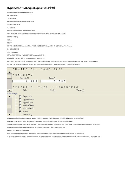
屈服极限为235Mpa。
下图为材料编辑的界⾯5.在card image中激活Density、Elastic和Plastic三个选项,并在Density中输⼊数值7.9E-6,设定弹性模量E为210,泊松⽐Nu为0.3。
6.将PLASTICDATACARD设为1,输⼊屈服应⼒0.235(Gpa),相应的塑性应变设为0.0。
点击return 退出材料编辑。
7.在collector/update⼦⾯板中设定操作对象为comp,选择名为box的component,并选择材料Q235,点击update。
在下⼀级菜单中选择material id,点击update。
- 1、下载文档前请自行甄别文档内容的完整性,平台不提供额外的编辑、内容补充、找答案等附加服务。
- 2、"仅部分预览"的文档,不可在线预览部分如存在完整性等问题,可反馈申请退款(可完整预览的文档不适用该条件!)。
- 3、如文档侵犯您的权益,请联系客服反馈,我们会尽快为您处理(人工客服工作时间:9:00-18:30)。
Hypermesh和Abaqus的接口分析实例(三维接触分析)In this tutorial, you will learn how to:✓Load the Abaqus user profile and model✓Define the material and properties and assign them to a component✓View the *SOLID SECTION for solid elements✓Define the *SPRING properties and create a component collector for it✓Create the *SPRING1 element✓Assign a property to the selected elementsStep 1: Load the Abaqus user profile and modelA set of standard user profiles is included in the HyperMesh installation. They include: RADIOSS (Bulk Data Format), RADIOSS (Block Format), Abaqus, Actran, ANSYS, LS-DYNA, MADYMO, Nastran, PAM-CRASH, PERMAS, and CFD. When the user profile is loaded, applicable utility menu are loaded, unused panels are removed, unneeded entities are disabled in the find, mask, card and reorder panels and specific adaptations related to the Abaqus solver are made.1. From the Preferences drop down menu, click User Profiles....2. Select Abaqus as the profile name.3. Select Standard3D and click OK.4. From the File drop down menu, select Open… or click the Open .hm file icon.5. Select the abaqus3_0tutorial.hm file.6. Click Open.Step 2: Define the material propertiesHyperMesh supports many different material models for Abaqus. In this example, you will create the basic *ELASTIC material model with no temperature variation. The material will then be assigned to the property, which is assigned to a component collector.Follow the steps below to create the *ELASTIC material model card:1. From the Materials drop down menu, select Create.2. Click mat name = and enter STEEL.3. Click type= and select MATERIAL.4. Click card image = and choose ABAQUS_MATERIAL.5. Click create/edit. The card image for the new material opens.6. In the card image, select Elastic in the option list.7. By default, the selected type is ISOTROPIC. If not, click the switch and select ISOTROPIC.8. By default, the ELASTICDATACARDS= field value is 1. If not, input 1 to set thenumber of datalines.9. Click the field beneath E(1) and enter 2.1E5.10.Click the field beneath NU(1) and enter 0.3.11.Click return to accept the changes to the card image.12.Click return to exit the panel.Step 3: Define the *SOLID SECTION properties1. From the Properties drop down menu, select Create.2. Click prop name= and enter Solid_Prop.3. Choose a color for the property.4. Click on type=and set it to SOLID SECTION. This ensures that sections pertaining only to solid elements are available as card image options. Alternatively, the type = field can be set to ALL ensuring that all available card images are listed.5. Click on card image= and select SOLIDSECTION.6. Click material= and select STEEL.7. Click create.8. Click return to exit the panel.Step 4: Assign the property to the componentBecause the material is assigned to the property, when you assign the property to a component, the material is automatically assigned as well.1.From the Collectors drop down menu, select Edit and select Components.2.Click the yellow comps button and select INDENTOR and BEAM from the list.3.Click select.4. If necessary, click the toggle to switch <property blank> to property= .5. Double-click property= and select the Solid_Prop.Notice that the card image= and material= are already set from the Solid_Prop property.6. Click update.7. Click return to exit the panel.Step 5: View the *SOLID SECTION for solid elementsHyperMesh supports sectional properties for all elements from the property collector.Complete the steps below to view the *SOLID SECTION card for an existing component:1. From the Properties drop down menu, select Card Edit.2. Click props and select Solid_Prop from the list of property collectors.3. Click select to finish the selection process.4. Click edit to view the *SOLID SECTION property card image.5. Click return to finish the viewing process.6. Click return to exit the panel.Step 6: Define the *SPRING propertiesIn Abaqus contact problems, it is common to use weakly grounded springs to provide stability to the solution in the first loading step. This section explains how to create these springs and how to create the *SPRING card.Complete the steps below to create the *SPRING card:1. From the Properties drop down menu, select Create.2. Click prop name= and type in Spring_Prop.3. Choose a color for the property collector.4. Click on type=and set it to LINE SECTION. This ensures that sections pertaining only to 1D elements are available as card image options. Alternatively, the type = field can be set to ALL ensuring that all available card images are listed.5. Click on card image= and select SPRING.6. Click material= and select STEEL.7. Click create/edit.8. In the dof1 field, enter 3.The dof2 field in the *SPRING card is ignored by Abaqus for SPRING1 elements.9. In the Stiffness field, enter 1.0E-5.10.Click return to accept the changes to the card image.11.Click return to exit the panel.Step 7: Create a component collector for the *SPRING property1. From the Collectors drop down menu, select Create and select Components.2. Click comp name= and type in GROUNDED.3. Choose a color for the property collector.4. If necessary, click the toggle to switch <property blank> to property= .5. Double-click property= and select the Spring_Prop.Notice that the card image = and material = are already set from the Spring_Prop property.6. Click create.7. Click return to exit the panel.To reset the view for further processing:1. Click the isometric view icon .Step 8: Create the SPRING1 element1. From the Mesh drop down menu, select Assign and select Element Type.2. In the 1D sub-panel, click mass = and select SPRING1.In HyperMesh, grounded elements are created and stored as mass elements since they only have one node in the element connectivity.3. Click return to exit the panel.4. On the status bar at the bottom of the window, the name of the current component is displayed. Click on that name.5. Select GROUNDED from the list of component collectors that appears.As the spring elements are created, they will be placed in this component.6. From the Mesh drop down menu, select Create and select Masses.7. Click nodes and select by id from the pop-up menu.8. In the id = field, enter 451t460b3 and click Enter on the keyboard.This shorthand selects all of the nodes from 451 to 460 in increments of 3.9. Click create.10.Click return to exit the panel.定义接触面和相互作用Step 9: Start the Contact Manager1. From the Utility menu, click the Contact Manager button.The Abaqus Contact Manager dialog opens.Step 10: Create the "Indentor-top" surface1. Select the Surface tab in the Abaqus Contact Manager dialog.2. Click the New… button.The Create New Surface dialog opens.3. In the Name: field, enter indentor-top.4. Select Element based as the type of surface.5. Click Color and select a color.6. Click Create….The Element Based Surface dialog opens for defining elements and corresponding faces for the surface.7. In the Model Browser, expand the Components folder to display all the contents. Right-click on indentor and select Isolate.8. Click the user views icon and select top.9. In the Element Based Surface dialog, select the Define tab.10.In the Define surface for: list, select 3D solid, gasket.11.Click the Elements button.This opens the element selector panel.12.Click the elems button.13.Select by collector.14.Check the indentor component and click select.You will see the elements in indentor component highlighted.15.Click proceed to return to the Element Based Surface dialog.16.Select Solid skin option from the Select faces by: radio buttons.17.Select a color from the Solid skin color: button.18.Click the Faces button.This creates a temporary skin of the selected elements and opens the element selector panel.19.Select an element from the top of the solid skin.20.Click the elems button and select by face.You will see all faces at the top of the solid skin are highlighted.21.Rotate the model in HyperMesh interface to verify all desired faces are selected.You can deselect any element (by right clicking) or add more if you like.22.When you are satisfied with the element faces selected, click proceed to return to the Element Based Surface dialog.23.Click the Add button to add these faces to the current surface.This creates special "face" elements (rectangles with dot in the middle) for display.You can reject the recently added "faces" by clicking the Reject button. You can also delete "faces" from the Delete Face page.24.When satisfied with the surface definition, click Close to return to the AbaqusContact Manager dialog.Step 11: Create the "Beam-bot" surface1. Select the Surface tab in the Abaqus Contact Manager dialog and click the Display None button to undisplay all surfaces.2. Click the New… button.This opens the Create New Surface dialog.3. In the Name: field, enter cylinder-top.4. Select Element based as the type of surface.5. Click the Color: button and select a color.6. Click Create….The Element Based Surface dialog opens for defining elements and corresponding faces for the surface.7. In the Model Browser, expand the Components folder to display all the contents. Right-click on Beam and select Isolate.8. In the Element Based Surface dialog, select the Define tab.9. In the Define surface for: list, select 3D solid, gasket.10.Click the Elements button.This opens the element selector panel.11.Click the elems button, select by collector, check Beam component and click select. This highlights the elements in Beam component.12.Click proceed to return to the Element Based Surface dialog.13.Select Solid skin from the Select faces by: radio buttons.14.Select a color from the Solid skin color: button.15.Click the Faces button.This creates a temporary skin of the selected elements and opens the element selector panel.16.Select an element from the solid skin, click the elems button, and select by face.You will see faces all around the solid skin are highlighted.17.Rotate the model in the HyperMesh interface to verify all desired faces are selected.You can deselect any element (by right clicking) or add more if you like.18.When you are satisfied with the element faces selected, click proceed to returnto the Element Based Surface dialog.19.Click the Add button to add these faces to the current surface.This creates special "face" elements (rectangles with dot at the middle) for display.You can reject the recently added "faces" by clicking the Reject button. You can also delete "faces" from the Delete Face page.20.When satisfied with the surface definition, click Close to return to the Abaqus Contact Manager dialog.Step 12: Define the surface interaction propertyIn this exercise, you will define the *SURFACE INTERACTION card with corresponding *FRICTION card.Complete the steps below to create the "friction1" surface interaction:1. Select the Surface Interaction tab at the Abaqus Contact Manager dialog.2. Click the New… button.This opens the Create New Surface Interaction dialog.3. In the Name: field, enter friction1.4. Click the Create… button.The Surface Interaction dialog opens.5. Select the Define tab.6. Select Friction option as surface interaction property.That makes the Friction tab active.7. Select the Friction tab.8. Select the Friction type: as Default and click the Direct option.Selecting this option means that the exponential decay and Anisotropic parameters will not be written to the input file.9. In the No of data lines field, enter 1 and click set.A single row appears in the Direct table.10.Click the first cell on the Friction Coeff column and enter 0.05. For Direct and Anisotropic tables:•The column numbers in the table will change with the No of Dependencies selected. The row numbers can be defined at the No of data lines entry box. Clicking the corresponding Set button will update the table to have the specified number of rows.•For placing values in the table, click a cell to make it active and type in the values. The table works like a regular spreadsheet.•You can also read comma-delimited data from a text file by clicking the Read From a File button. This button opens up a file browser window. Select the file and click Open to export the comma-delimited data. The row number will be set to the number of data lines found in the file.•Right-clicking in the table shows a pull down menu with copy, cut and paste options. Comma-separated data can be copied/cut into or pasted from clipboard with these options. Relevant hot keys (for example, Ctrl-c, Ctrl-x and Ctrl-v in Windows) will also work.•Clicking the left mouse button in a cell activates that cell. Clicking into an already active cell moves the insertion cursor to the character nearest the mouse.•Moving the mouse while the left mouse button is pressed highlights a selected area.•The left, right, up and down arrows moves the active cell.•Shift-<arrow> extends the selection in that direction.•Ctrl-left arrow and Ctrl –right arrow move the insertion cursor within the cell.•Ctrl -slash selects all the cells.•Back space deletes the character before the insertion cursor in the active cell. If multiple cells are selected, Back space deletes all selected cells.•Delete deletes the character after the insertion cursor in the active cell. If multiple cells are selected, Delete deletes all selected cells.•Ctrl -a moves the insertion cursor to the beginning of the active cell. Ctrl-e moves the insertion cursor to the end of the active cell.•Ctrl –minus (-) and Ctrl –equal (=) decrease and increase the width of the column with the active cell in it.•To interactively resize a row or column, move the mouse over the border while Button-1 or Button-3 (the right button on Windows) is pressed.11.Click OK to return to the Abaqus Contact Manager dialog.Step 13: Create the "Beam-Indentor" contact pair1. Go to the Interface tab of the Abaqus Contact Manager dialog.2. Click the New… button.This opens the Create New Interface dialog.3. In the Name: field, enter Beam-indentor.4. Select Contact pair as the type of interface.5. Click the Create… button.The Contact Pair window opens.6. Select the Define tab.7. Click the Surface: pull down menu to show a list of the existing surfaces.8. Select indentor from the list and click the Slave>> button to identify it as theslave surface and move it into the table.9. Click the corresponding Review button.The selected surface is highlighted in red. If the surface is defined with sets (display option disabled), the underlying elements are highlighted. Right-click on Review to clear the highlighting.The corresponding New button opens the Create New Surface dialog for creating a new surface. When you are done creating and defining the surface, the Contact Pair window returns with the new surface selected as the slave surface.10.Repeat steps 7 and 8, selecting Beam and clicking the Master>>button to identify it as the master surface.Note: To more clearly see the surfaces available for selection, click the icon.This opens an enhanced browser where you can easily search for the appropriate item. You can also click the Filter button to filter the items displayed.11.Click the Interaction: drop down list to see a list of the existing surfaceinteractions.Note: To more clearly see the interactions available for selection, click theicon. This opens an enhanced browser where you can easily search for the appropriate item. You can also click the Filter button to filter the items displayed.12.Select friction1from the list as the interaction property for the current contactpair.13.Select the Parameter tab.14.Select SmallSliding from the available options.15.Click OK to return to the Abaqus Contact Manager dialog.16 Click close to the Abaqus Contact Manager dialog.创建载荷和边界条件Step 14: Define a *STEP card and specify *STATIC as the analysis procedureIn this exercise, you will create a *STEP card with the *STATIC analysis procedure.1. On the Utility tab, click Step Manager.The Step Manager dialog is displayed.2. Click New…3. In the Name: text box enter step1.4. Click Create to create the step.This creates a step called step1 and opens the Load Step edit dialog.5. From the tree on the left side of the window, select Title.The Step heading: option with a disabled field is displayed.6. Activate the Step heading: check box and enter 100kN load in the text box.7. Click Update to store the heading information into step1.8. From the tree, select Parameter.9. Activate the Name and Perturbation check boxes, and click Update. Notice that name is already set to step1.10.From the tree, select Analysis procedure.11.For Analysis type:, select static and click Update.In this exercise, you created a step (*STEP) called step1 and specified *STATIC as the analysis procedure.12.To add a dataline, go to the Dataline tab and enable Optional dataline.13.To add individual data, such as Initial increment, enable the appropriate field and enter a value. If one entry field is not enabled, a space will be added in the ASCII file, and the Abaqus solver uses the default value.Next, you will define the loads and boundary conditions. Step 15: Create constraints (*BOUNDARY)1. From the tree, select Boundary.2. Click New… and enter loads_and_constraints in the Name: text box.3. Click Create to create the load collector.4. Optionally, click the button in the Display column and select a color for the load collector.5. Make sure the Status check box for loads_and_constraints is checked. By selecting this check box, you are adding this load collector into the loadstep.6. Click the loads_and_constraints load collector in the table.A set of new tabs is displayed on the right.7. From the Define tab, keep Type: set to default (disp).8. Click the Define from ‘Constraints’ panel button.This takes you to the Constraints panel in HyperMesh. Use this panel to create constraints.Step 16: Create constraints from the Constraints panel1. On the toolbar, click the user views icon and select right.2. Click the yellow nodes button and select by sets.3. select ENDS then Click select buttom.4. Activate dof1, dof2, dof3, unactivate dof4, dof5, dof6.5. Click create.HyperMesh creates constraints at the nodes you selected.6. Click return.You are returned to the Step Manager Load Step dialog.7. Look at the Load type: line at the bottom of the Step Manager dialog. Notice thatBc (short for BOUNDARY) appears on this line, identifying it as a load type created in the load_and_constraints load collector. The corresponding load type on the tree is also highlighted.Step 17: Create Forces (*CLOAD)1. From the tree, double-click Concentrated loads.2. Select CLOAD-Force from the expanded options under Concentrated loads.3. Click New… and enter 100KN_loaded in the Name: text box.4. Click Create to create the load collector.5. Optionally, click the button in the Display column and select a color for the load collector.6. Make sure the Status check box for 100KN_loaded is checked. By selecting this checkbox, you are adding this load collector into the loadstep.7. Click the 100KN_loaded load collector in the table.A new set of tabs is displayed.8. From the Define tab, define CLOAD_Force on: Nodes or geometry.9. From Define tab, click Define from ‘Forces’ Panel.The HyperMesh Forces panel is displayed. Use this panel to create forces. Step 18: Create forces from the Forces panel1. From the graphics area, click the central node on the front side of the indentor.2. In the magnitude: text box, enter –100 kN.3. Click the switch next to N1, N2, N3 and select Y-axis.4. Click create.5. Click return.You are returned to the Step Manager Load Step dialog.6. Notice that Cload-f is now added to the Load type: line, indicating CLOAD-force as another load type created in the loads_and_constraints load collector. The corresponding load types on the tree are also highlighted.7. From the Load Step dialog, left-click Review.The constraints and forces that belong to the loads_and_constraints load collector are highlighted.8. Right-click Review.The highlighted constraints and forces revert back to the load collector color. Steps 19-20: Define Output Requests(定义输出)In this exercise, you will specify several output requests for step1. There are two methods for defining output request described below.Step 19: Request ODB file outputs1. From the tree, double-click Output request.2. Select ODB file from the expanded options under Output request.3. Click New… and enter step1 output in the Name: text box.4. Click Create.5. Click step1 output (which you just created).A new set of tabs is displayed on the right.6. From the Output tab, activate the Output check box. Leave Output set to field.7. Activate the Node output and Element output options.The Node Output and Element Output tabs are activated.8. Click the Node Output tab.9. Click Displacement and activate the U check box.U is added to the data line on the right. You are now requesting displacement results in the ODB file.Note: You can manually type in an output request into this table, including unsupported requests. They will be written out as entered in the table.10.Click Update.11.Click the Element Output tab.12.Activate the Position check box and set it to Nodes.13.Click Stress and activate the S check box.S is added to the data line on the right. You are now requesting stress results in the ODB file.14.Click Update.Step 20: Request results file (.fil) outputs1. From the tree, under Output request, select Result file (.fil).2. From the Define tab, activate the Node file and Element file check boxes.The Node File and Element File tabs are activated.3. From the Node Fi le tab, in the lower left area, expand Displacement and activate U.U is added to the data line on the right. You are now requesting displacement results in the .fil file.4. Click Update5. From the Element File tab, activate the Position check box and set it to averaged at nodes.6. In the lower left area, double-click Stress and activate S.S is added to the data line on the right. You are now requesting stress results in the .fil file.7. Click Update.8. Click Review.A text-editor showing the output requests you made is displayed. This is the format used in the Abaqus input file (.inp).9. Click Close on the text-editor window.10.Click Close.The Load Step edit dialog of Step Manager closes and you are returned to the main Step Manager dialog. The main Step Manager dialog displays step1 information as we defined in previous exercises.11.Click Close to exit the Step Manager dialog.Steps 21-22: Export the database to an Abaqus input fileThe data currently stored in the database must be output to an Abaqus .inp file for use with the Abaqus solver. The .inp file can then be used to perform the analysis using Abaqus outside of HyperMesh.Step 21: Export the .inp file1. From the F ile drop down menu, select E xport....2. In the File: field, enter job1.inp.3. Click the Export Options down arrows.4. Click the Export: toggle to all.5. Click Apply.6. Click Close to close the Export panel.Step 22: Save the .hm file and quit HyperMesh1. From the F ile drop down menu, select S ave as….2. Select your working directory and for File name:, enter job1.hm.3. Click Save.4. From the F ile drop down menu, select Exit.。