Surface latent heat flux anomalies preceding inland earthquakes in China

合集下载

【SMT资料】profile 对reflow制程的影响

ppt课件
27
現在我們來討論為甚麼“馬鞍型溫度曲線”被廣泛使用的理由，主要是因為透過強迫性對流流焊製程的協助，有恆溫區的加溫曲線可達到類似在汽相流焊製程中的最高流焊區極上熱平衡分佈的結果。
我們認為要達到最佳的產品產出率，在考慮如何決定流焊的溫度曲線時，因此考慮各種不同零件的吸熱情況以及底材PCB的特性而不必太在乎加熱製程中錫膏的表現。
* In order to overcome the problem, the momentum relation must become as below ;
T1 + T2 ＜T3
T1 + T2 ≧T3
T3
d
T1 T2
Partial melting
ppt课件
9
Reflow Zone :
*Peak temperature and Reflow time should be controlled
ppt课件
11
如何改善錫球
鋼板內距
0603 0.7 ~0.8mm 0808 1.1 ~1.2mm 12.6 1.95~2.1mm
鋼板形狀
ppt课件
12
ppt课件
13
Reflow後造成的坍塌
升溫速度過快 Soften Point Slump resistivity PAD間文字面的白漆，或Trace線
ppt课件
25
由於業界對P.C板輕溥短小的設計的改進， SMT零件的分佈密度愈趨緊密，加速了高熱含量零件封裝體的應用，例如IC和 QFP。因為各種不同大小零件間的熱含量增加，使得在使用傳統的遠紅線(far IR) 流焊爐時，因為熱量分佈不均，再加上使用“和緩溫昇型”的溫昇曲線(甚至於 “馬鞍狀，恆溫型溫度曲線”)，很難在零件間達到熱平衡。

Ti离子注入和退火对ZnS薄膜结构和光学性质的影响

Ti 离子注入和退火对ZnS 薄膜结构和光学性质的影响1苏海桥1，薛书文2，陈猛1，李志杰1，袁兆林1，付玉军3，祖小涛11 电子科技大学应用物理系，成都（610054）2 湛江师范学院物理系，湛江（524048）3 兰州大学物理科学与技术学院，兰州（730000）E-mail ：xtzu@摘要：利用真空蒸发法在石英玻璃衬底上制备了ZnS 薄膜，将能量80keV ，剂量1×1017ions/cm 2的Ti 离子注入到薄膜中，并将注入后的ZnS 薄膜进行退火处理，退火温度从500到700℃。

利用X 射线衍射(XRD)研究了薄膜结构的变化，利用光致发光(PL)和光吸收研究了薄膜光学性质的变化。

XRD 结果显示，衍射峰在500℃退火1小时后有一定程度的恢复；光吸收结果显示，离子注入后光吸收增强，随着退火温度的上升，光吸收逐渐降低，吸收边随着退火温度的提高发生蓝移；光致发光显示，薄膜发光强度随退火温度的上升而增强。

关键词：ZnS 薄膜；离子注入；XRD ；光致发光中图分类号：6180J, 7155G1．引言ZnS 是一种重要的II-VI 族宽禁带半导体材料（禁带宽度约3.65eV ），广泛应用于光电器件中，如蓝光发射二极管，薄膜电致发光设备，太阳能电池窗口材料[1–4]。

制备高质量ZnS 薄膜的方法有很多，包括溅射法[5]，分子束外延 [6]，激光脉冲沉积[7]，化学气相沉淀 [8]，化学浴沉淀 [9]，真空蒸发法 [10–12]等。

蒸发法的特点是所制得纳米薄膜表面清洁，成膜粒子的粒径可通过加热温度、压力等参数来调控。

而且制作方便，对仪器要求不苛刻，成膜速度快。

掺杂可以改变材料的物理化学性质，可以扩展其应用范围。

离子注入是半导体掺杂的主要方式，在半导体工业中应用极为广泛。

它的优点是可以进行选区掺杂，不受掺杂物固溶度的影响，并能精确控制掺杂物的浓度。

理论上，每一种元素都可以利用离子注入技术进行掺杂，因此，它是一种十分灵活和便利的掺杂技术。

Latent heat and specific heat capacity

Latent heat of vaporization
The heat required to change a 1.0 kg of substance from the liquid to the vapor phase is called the heat of vaporization, Lv.
Specific heat capacity
where c is a quantaterial called its specific heat.
Latent heat of fusion
The heat required to change 1.0 kg of a substance from the solid to the liquid state is called the heat of fusion; it is denoted by LF
Thermodynamics: a subject to investigate relation among temperature, internal energy and heat.
Distinguishing Temperature, Heat, and Internal Energy
Temperature (in kelvins) is a measure of the average kinetic energy of individual molecules
Internal energy refers to the total energy of all the molecules within the object
Heat, finally, refers to a transfer of energy from one object to another, which is energy transferring on the way.

2011 ENSO and Indian Ocean sea surface temperatures

2
A. J. MANHIQUE ET AL.
Figure 1. Satellite images showing cloud bands typical of TTTs over southern Africa on 2nd and 7th December 2005 (courtesy of the Mozambique Institute of Meteorology).
of opposite sign in the Southwest and southeast Indian Ocean. Positive rainfall anomalies tend to be observed when the warm (cool) pole is located in the west (east) of the subtropical South Indian Ocean (Reason, 2001, 2002). Fauchereau et al. (2003) and Hermes and Reason (2005) showed that this SIOD can often occur at the same time as a similar dipole in the South Atlantic and South Paciﬁc Oceans and is related to surface heat ﬂux anomalies generated by modulations to the atmospheric wavenumber-3 or -4 pattern in the mid-latitude Southern Hemisphere. Tropical temperate troughs (TTTs – Figure 1 shows examples of the cloud bands associated with these systems) have been recognised as the main summer synoptic rain-producing systems over southern Africa (Harrison, 1984; Washington and Todd, 1999; Tyson and PrestonWhyte, 2000; Reason et al., 2006). Collectively over the austral summer, they contribute to the South Indian convergence zone (SICZ – Cook, 2000). However, the mechanisms that inﬂuence either the frequency of occurrence of these systems over southern Africa or their intensity are not well understood. The signiﬁcant relationship between rainfall over southern Africa and SST patterns in the South Indian Ocean may imply that these

热退火对InGaN薄膜性质的影响

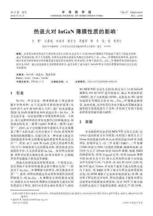
行比较，用蓝宝石（衍射峰作为基准进行了归０００２）一化．从比较结果可以看到，样品衍射峰强度在４００和４而在５５０℃ 下退火并没有明显变化，００℃ 下退火后，这意味着晶格犐狀犪０．１４犌０．８６犖的衍射峰有所增强，质量有所提高．５５０℃ 退火后，犐狀犪０．１４犌０．８６犖的衍射峰显著下降，意味着在此温度下退火晶格质量显著退化．图２所示的１犿×１犿的犃犉犕图像为典型的 μ μ （）、（、（）分别对犐狀犪犪犫）犮０．１４犌０．８６犖薄膜的表面形貌，退火后的样品和应于未退火的样品、５００℃ ５５０℃ 退火后的样品．图像中台阶纹清晰可见，说明犐狀０．１４薄膜处于二维生长模式样品的均方根粗犌犪．０．８６犖分别为０另糙度（犚犕犛）７３６，０５８６和１２２３狀犿．图中还清楚地观察到了犞型缺陷，它们是由薄外，膜中的线位错和应力释放过程中产生的层错诱发形］１０～１２成的［在（）、（）、（）三个样品中的犞型缺陷．犪犫犮９９９和２密度分别为１３×１０，０８×１０５×１０犮犿－２．犚犕犛和犞型缺陷密度随退火温度的变化关系以及犡犚犇的测量结果都证明了５００℃ 是退火的一个最这是因为在５下退火时，热能为原子的佳温度．００℃ 重新排列提供了足够的驱动力，使其晶格排列得更从而减少了晶体中的缺陷、位错、层错，提高加整齐，了晶体的质量．但是在更高的温度下退火时，由于在５犐狀犌犪犖中的犐狀—犖键的键能很低，５０℃ 时已经开始断裂，导致薄膜中的犐晶体质狀犌犪犖开始分解，量显著恶化．

Sensitivity studies on the impacts of Tibetan Plateau

Atmos.Chem.Phys.,11,1929–1948,2011 /11/1929/2011/ doi:10.5194/acp-11-1929-2011©Author(s) Attribution3.0License.Atmospheric Chemistry and PhysicsSensitivity studies on the impacts of Tibetan Plateau snowpack pollution on the Asian hydrological cycle and monsoon climateY.Qian1,M.G.Flanner2,L.R.Leung1,and W.Wang31Paciﬁc Northwest National Laboratory,Richland,W A,USA2University of Michigan,Ann Arbor,MI,USA3NOAA National Centers for Environmental Prediction,Camp Springs,MD,USAReceived:27August2010–Published in Atmos.Chem.Phys.Discuss.:5October2010Revised:21January2011–Accepted:16February2011–Published:2March2011Abstract.The Tibetan Plateau(TP)has long been identiﬁedto be critical in regulating the Asian monsoon climate andhydrological cycle.In this modeling study a series of numer-ical experiments with a global climate model are designedto simulate radiative effect of black carbon(BC)and dustin snow,and to assess the relative impacts of anthropogenicCO2and carbonaceous particles in the atmosphere and snowon the snowpack over the TP and subsequent impacts on theAsian monsoon climate and hydrological cycle.Simulationsresults show a large BC content in snow over the TP,espe-cially the southern slope.Because of the high aerosol contentin snow and large incident solar radiation in the low latitudeand high elevation,the TP exhibits the largest surface radia-tiveﬂux changes induced by aerosols(e.g.BC,Dust)in snowcompared to any other snow-covered regions in the world.Simulation results show that the aerosol-induced snowalbedo perturbations generate surface radiativeﬂux changesof5–25W m−2during spring,with a maximum in April orMay.BC-in-snow increases the surface air temperature byaround1.0◦C averaged over the TP and reduces spring snow-pack over the TP more than pre-industrial to present CO2in-crease and carbonaceous particles in the atmosphere.As a re-sult,runoff increases during late winter and early spring butdecreases during late spring and early summer(i.e.a trendtoward earlier melt dates).The snowmelt efﬁcacy,deﬁned asthe snowpack reduction per unit degree of warming inducedby the forcing agent,is1–4times larger for BC-in-snow thanCO2increase during April–July,indicating that BC-in-snowmore efﬁciently accelerates snowmelt because the increasednet solar radiation induced by reduced albedo melts the snowmore efﬁciently than snow melt due to warming in theair.Correspondence to:Y.Qian (yun.qian@)The TP also inﬂuences the South(SAM)and East(EAM) Asian monsoon through its dynamical and thermal forcing. Simulation results show that during boreal spring aerosols are transported by southwesterly,causing some particles to reach higher altitude and deposit to the snowpack over the TP.While BC and Organic Matter(OM)in the atmosphere directly absorb sunlight and warm the air,the darkened snow surface polluted by BC absorbs more solar radiation and increases the skin temperature,which warms the air above through sensible heatﬂux.Both effects enhance the upward motion of air and spur deep convection along the TP dur-ing the pre-monsoon season,resulting in earlier onset of the SAM and increase of moisture,cloudiness and convective precipitation over northern India.BC-in-snow has a more signiﬁcant impact on the EAM in July than CO2increase and carbonaceous particles in the atmosphere.Contributed by the signiﬁcant increase of both sensible heatﬂux asso-ciated with the warm skin temperature and latent heatﬂux associated with increased soil moisture with long memory, the role of the TP as a heat pump is elevated from spring through summer as the land-sea thermal contrast increases to strengthen the EAM.As a result,both southern China and northern China become wetter,but central China(i.e. Yangtze River Basin)becomes drier–a near-zonal anomaly pattern that is consistent with the dominant mode of precipi-tation variability in East Asia.The snow impurity effects reported in this study likely rep-resent some upper limits as snowpack is remarkably overesti-mated over the TP due to excessive precipitation.Improving the simulation of precipitation and snowpack will be impor-tant for improved estimates of the effects of snowpack pollu-tion in future work.Published by Copernicus Publications on behalf of the European Geosciences Union.1IntroductionSnow albedo is important in determining the surface energy transfer within the cryosphere.One factor that affects snow albedo is the presence of absorbing particles (e.g.soot,dust)(Warren and Wiscombe,1980,1985;Painter et al.,2007).The visible snowpack albedo can be reduced from 0.95for pure snow to 0.1for dirty snow with 100ppm by weight (ppmw)of soot (Warren and Wiscombe,1980).Although estimates of present-day global-mean radiative forcing (RF)from soot in snow are only ∼0.04–0.20W m −2,the local RF could be much higher.Climate models suggest this mecha-nism has greater efﬁcacy than any other anthropogenic agent (Hansen and Nazarenko,2004;Jacobson,2004;Hansen et al.,2005;Flanner et al.,2007;Qian et al.,2009a),owing largely to its effectiveness in removing snow cover.The 2007IPCC report listed the radiative forcing induced by “soot on snow”as one of the important anthropogenic forcings affect-ing climate change.It is important to understand the control of snow cover evolution because most of the interannual vari-ability in mid-and high-latitude planetary albedo is caused by changes in snow and sea-ice cover (Qu and Hall,2006).Modeling studies have shown that the long-term average of snow accumulation or melt patterns may signiﬁcantly alter global and regional climate and have a strong impact upon the general circulation and hydrological cycle (e.g.,Barnett et al.,1988;Qian et al.,2009a).The Tibetan Plateau (TP)is the highest and largest plateau in the world.It covers an area of 3.6million km 2at 2000m above the mean sea level (MSL)(see Fig.1).Glaciers on the TP hold the largest ice mass outside the Polar region and the snowpack can persist year round at higher altitude regions over the TP (Xu et al.,2009;Pu and Xu,2009).The TP has long been identiﬁed to be critical in regulating the Asian hydrological cycle and monsoon climate (e.g.Yanai et al.,1992;Wu and Zhang,1998;Xu and Chan,2001).First,the glaciers over the TP act as a water storage tower for South Asia,Southeast Asia and East Asia.Precipitation and re-leased melt water from the TP provide fresh water to billions of people through the major rivers that originate from the TP.For example,the glacial and snow melt provides up to two-thirds of the summer ﬂow in the Ganges and half or more of the ﬂow in other major rivers (Qin et al.,2006).The long-term trend and/or seasonal shift of water resource provided by the TP may signiﬁcantly affect agriculture,hydropower and even national security for the developing countries in the region.Second,thermal heating of the TP has profound dynami-cal inﬂuences on the atmospheric circulation in the Northern Hemisphere (Manabe and Terpstra,1974;Yeh et al.,1979).Anomalous snow cover can inﬂuence the energy and water exchange between the land surfaces and the lower tropo-sphere by modulating radiation,water and heat ﬂux (Cohen and Rind,1991).Lau and Kim (2006)and Lau et al.(2006)proposed a so-called Elevated Heat Pump (EHP)effect,Fig.1.Terrain of Tibetan Plateau (Unit:m).whereby heating of the atmosphere by elevated absorbing aerosols strengthens local atmospheric circulation,leading to a northward shift of the monsoon rain belt,with increased rainfall in northern India and the foothills of the Himalayas in the late boreal spring and early summer season.Although Nigam and Bollasina (2010)showed that there is little ob-servational evidence that supports the EHP because the ob-served aerosol and precipitation anomalies are in fact not col-located,their analysis of hydroclimate lagged regressions on aerosols suggests that precipitation anomalies in Northern In-dia can be interpreted as impacts of aerosols,rather than an aerosol-precipitation relationship due to aerosol removal by u and Kim (2011)argued that validation of the EHP has to be based on the forcing and response of the entire monsoon system from pre-onset to termination,and not based on local correlation of aerosol and rainfall at one time.Meanwhile,many studies based on modeling and ob-servational data analysis have found a remarkable relation-ship between the winter or spring snow over the TP and rain-fall over the mid-and lower-reaches of the Yangtze River Basin (YRB)in eastern China and South China in the sub-sequent summer (e.g.Wu and Qian,2003;Qian et al.,2003;Zhang et al.,2004),primarily through two important effects of snow cover –inﬂuence on surface albedo and soil moisture (Barnett et al.,1989;Yasunari et al.,1991).Observational evidence indicates that the surface tempera-tures on the TP have increased by about 1.8◦C over the past 50years (Wang et al.,2008).IPCC 2007reported that under the A1B emissions scenario,a 4◦C warming will likely oc-cur over the TP during the next 100yr (Meehl et al.,2007).Both observed and projected warming over the TP is much larger than the global average.Consequently,the glaciers on the TP have been retreating extensively in past decades (Qin et al.,2006).In the short term,this will cause lakes to expandAtmos.Chem.Phys.,11,1929–1948,2011/11/1929/2011/and bringﬂoods and mudﬂows.In the long run,the glaciers are vital lifelines for Asian rivers such as the Indus and the Ganges.Once they vanish,water supplies in those regions will be in peril.Accelerated melt of global snowpack and glaciers is driven by warming due to increasing greenhouse gases(GHGs) (Barnett et al.,2005),but the larger rate of warming and ra-pidity of glacier retreat suggest that additional mechanisms may be involved(Xu et al.,2009).The TP is located close to regions in South and East Asia that have been and are pre-dicted to continue to be the largest sources of BC in the world (Bond et al.,2006;Menon et al.,2010).For example,the In-dian sub-continent,especially the Indo-Gangetic Plain,is one of the largest BC emission sources in the world(Ramanathan et al.,2007).Although the Himalayas may inhibit transport from the Gangetic Plain to the TP,some BC is transported and deposited to snow in the Himalayas and TP.Himalayan ice core records indicate a signiﬁcant increase in deposition of both BC and OC over the northern slope of the TP,espe-cially since1990(Ming et al.,2008;Xu et al.,2009).In contrast to the more straightforward radiative effects of GHGs in the atmosphere,atmospheric particles inﬂuence the snowpack energy budget in more complicated ways via sev-eral mechanisms(Flanner et al.,2009).First,through ab-sorption and scattering,aerosols reduce downwelling inso-lation at the surface(dimming)(e.g.,Ogren and Charlson, 1983;Qian et al.,2006),thus decreasing absorbed solar en-ergy by snowpack.Second,absorbing particles(e.g.soot) may warm the troposphere via solar heating.Recent ob-servational studies attributed the accelerated warming of the troposphere over the TP to atmospheric heating by aerosols (Gautam et al.,2009a,b;Prasad et al.,2009).Ramanathan et al.(2007)suggest that brown clouds contribute as much surface air warming over the Himalayas as anthropogenic greenhouse gases.This warming may transfer thermal en-ergy into snow and drive earlier melt,but may also stabi-lize the atmosphere and reduce surface-air energy exchange. Based on GCM experiment,Lau et al.(2010)ﬁnd that at-mospheric heating by black carbon and dust can induce a reduction of the Himalayan and Tibetan snowpack cover by 6–10%,without greenhouse warming.Third,deposited par-ticles(e.g.soot)reduce snow reﬂectance(surface darkening), counteracting the dimming effect.BC measurements in Mt. Everest ice core show mixing ratios that produced a summer darkening effect of4.5W m2in2001(Ming et al.,2008). The surface darkening caused by dirty snow may be magni-ﬁed with the snow aging process,which can be accelerated under warmer climate.In this study,we simulate the deposition and concentration of black carbon(BC)and dust over the TP,and calculate their radiative effect(i.e.,impact on surface radiativeﬂux changes, SRFC).We strive to understand the relative and combined impacts of anthropogenic CO2and carbonaceous particles in the atmosphere and snow on the snowpack over the TP, as well as their subsequent impacts on the Asian monsoon climate and hydrological cycle,based on a series of global climate simulations with various combinations of active car-bonaceous aerosols and CO2.Carbonaceous aerosol effects can be active or inactive in the atmosphere and in snow in the simulations,respectively,and the effect of different CO2 concentration is also simulated and compared with that for the aerosols.Our analysis focuses on the change of spring-time snowpack over the TP and their subsequent impacts on the SRFC and hydrological cycle(Sect.3)and summer mon-soon climate over the India and East Asia(Sect.4).2Model evaluation and experiments design2.1Model and experimentsEquilibrium global climate model(GCM)experiments were conducted with the National Center for Atmospheric Re-search(NCAR)Community Atmosphere Model version 3.1(CAM)(e.g.,Collins et al.,2006)with resolution ∼2.8◦×2.8◦near the equator.These simulations applied a slab ocean model to allow for fast equilibration,and were forced with constant greenhouse gas levels and monthly-varying,annually-repeating concentrations of mineral dust, sulfate,and sea-salt from an assimilation(Collins et al., 2001).BC and organic matter(OM)were treated prognos-tically(Rasch et al.,2000,2001),with annually-repeating emissions(i.e.,varying by month but identical each year) from a global1◦×1◦inventory(Bond et al.,2004),rep-resenting the values at1996.Emissions of organic carbon from this inventory were multiplied by1.4to represent or-ganic matter.This OM:OC ratio is appropriate for fossil OC emissions(Russell,2003).Biofuel and biomass burning emissions can contain higher ratios.The prescribed biomass burning OM emissions(and hence OM:OC ratios)vary with vegetation type(van der Werf et al.,2006).Hydrophobic species were transformed to hydrophilic with an e-folding time of1.2days.BC optical properties were modiﬁed to con-form to Bond and Bergstrom(2006),and include an absorp-tion enhancement factor of1.5for coated hydrophilic parti-cles(Bond et al.,2006).Optical properties for OM(Hess et al.,1998)include dependence on local relative humidity. The OM effect in snow is very small based on the sensitivity experiments we did,so we simply turned it off in this study. BC and mineral dust in snow were treated with the Snow, Ice,and Aerosol Radiative(SNICAR)component of CAM, described by Flanner et al.(2007,2009).We also apply the representation of snow cover fraction(Niu and Yang,2007), dependent on snow depth and density,that is included CLM 4.0.The BC content in snow follows from the simulated life-cycle of BC,starting with emissions.Hence,our deﬁni-tion of BC is identical to that used in Bond et al.(2004) in developing the emission inventories,namely:“the mass of combustion-generated,sp2-bonded carbon that absorbs/11/1929/2011/Atmos.Chem.Phys.,11,1929–1948,2011Table1.Model experiments.Experiment CO2FF+BF BC+OM a FF+BF BC BB BC+OM and dust b BB BC and dust bCase(ppm)active in atmos.?active in snow?active in atmos.?active in snow?pi1c289no no no nopi2380no no no nopi3289yes no no nopi4289no yes no nopi6380yes yes no nopd1d380yes yes yes yesa Fossil fuel and biofuel black carbon and organic matter.b Biomass burning black carbon and mineral dust.c pi is initialized with pre-industrial climate.d pd applies present-day boundary conditions and CO2level.the same amount of light as the emitted particles”.Thus, the simulated BC is indeed refractory-like,but is meant to account for an identical amount of light absorption as the emitted refractory BC and colored organics.Dust was not the focus of this study,but we included dust in experiment pd1to achieve a more realistic simulation.Prognostic dust emissions are based on the Dust Entrainment and Deposi-tion Model(Zender et al.,2003),and advected in4bulk size bins.Dust emissions are prognostic,and depend on local soil moisture,surface wind speed,soil erodibility,and veg-etation.Hence model dust emissions vary seasonally and inter-annually.Dust processes in this version of CAM are summarized in Mahowald et al.(2006).The visible single-scattering albedo values assumed for the four size bins of dust in snow range from0.88(largest size)to0.99(smallest size),as mentioned in Flanner et al.(2009).In the experi-ment pd1the dust is included together with Biomass Burn-ing(BB)BC and OM,so dust effect cannot be isolated in the current experiment design.Conﬁgurations of model experiments are described in Ta-ble1.These experiments were designed to assess the rel-ative climate impacts of anthropogenic CO2and carbona-ceous particles in the atmosphere and snow,and are a sub-set of those experiments described by Flanner et al.(2009). Experiments tagged“pi”were initialized with pre-industrial climate,whereas experiment pd1applied present-day bound-ary conditions.Experiment pi1is a control simulation,with pre-industrial CO2levels and BC+OM inactive in the atmo-sphere and snowpack.Experiment pi2applies modern CO2 levels(380ppm),but maintains inactive carbonaceous par-ticles.Experiment pi3maintains pre-industrial CO2levels, but includes active fossil and biofuel sources of BC+OM in the atmosphere.Experiment pi4also maintains pre-industrial CO2levels,but includes active fossil and biofuel sources of BC in the snow.Experiment pi6introduces all three forc-ing mechanisms(modern CO2,active BC+OM in atmo-sphere and BC in snow).Finally,experiment pd1applies full modern conditions,including all sources of carbonaceous particles(fossil,biofuel,and biomass burning)and mineral dust active in both the atmosphere and snowpack.Biomass burning BC+OM emissions applied in pd1were1997–2006 mean emissions from the Global Fire Emissions Database (van der Werf et al.,2006),version2(GFEDv2).In all equilibrium experiments,results were averaged over the last15yr of the50-yr simulations,during which the TOA net energyﬂux showed no signiﬁcant trend.So we are giv-ing the system35yr to equilibrate.Statistical difference be-tween the simulations was determined with two-sided pooled t-tests,using realizations from each of the15analysis years. Since the climate had equilibrated by the beginning of the 15-yr period,each year is treated as an independent sample of the equilibrium state.Thus,statistical signiﬁcance is de-ﬁned relative to the inherent inter-annual variability in the model.2.2EvaluationTo simulate the impacts of aerosol-induced snow albedo change,it is important to assess the basic features of the simulated climatic variables,especially the snowpack and the aerosol content in snow.A more detailed evaluation for CAM3performance in simulating the climate variables can be found in Collins et al.(2006).Here we just give a brief comparison of the measured and CAM-simulated snow cover fraction and BC content in snow over the TP.Controlled by precipitation and complex terrain over the TP,snow cover fraction(SCF),as retrieved from the Moderate Resolution Imaging Spectrometer(MODIS)and shown in Fig.2,ex-hibits an extremely inhomogeneous spatial distribution,with higher SCF in the mountain ranges(Pu and Xu,2009).The most persistent snow-covered areas(i.e.SCF>50%)are lo-cated over the Himalayas,Karakoram,Kunlun ranges and the western part of the Yarlung Zangbo Valley,especially the conjunction areas between the Karakoram and Kunlun glacier mountains with more than70%of snow/ice covered days annually.In the southeast TP,the SCF is also higher because of heavy precipitation resulting from the abundant moisture of the Yarlung Zangbo Valley.Due to rain shadowAtmos.Chem.Phys.,11,1929–1948,/11/1929/2011/Fig.2.Snow Cover Fraction(SCF)averaged for March-April-May (MAM)over Tibetan Plateau,(top)MODIS and(bottom)Model. effect from the Himalaya and Karakoram mountains,the SCF is smaller over the interior area of the TP,although the average elevation is above4000m.During summer,snow covered areas are more scattered.The CAM3remarkably overestimates the SCF,especially over the interior of the TP, due to its apparent inability to capture rainshadow effects of the massive plateau.Due to the coarse spatial resolution, CAM3fails to capture the complex terrain that generates the observed spatial variability of SCF.Figure3a shows the monthly mean SCF and snow water equivalent(SWE)from model and SCF from MODIS.The observation shows around25–35%of areas are covered by snow during winter and spring over the TP.The model over-predicts SCF by20–100%from November to April,but un-J F M A M J J A S O N DMonth20406080100SnowCoverFraction(%)(a)SCF modelSCF obsSWE20406080100SWE(mm)J F M A M J J A S O N DMonth2468Precipitation(mm/day)(b)modelFHQCRUUDELJ F M A M J J A S O N DMonth1234BCdeposition(x1-12kg/m2/s)(c)Dry+WetDryWetBC mass246810BCmassoversnow(x1-7kg)J F M A M J J A S O N DMonth123Dustdeposition(x1-9kg/m2/s)(d)Dry+WetDryWetFig.3.(a)Monthly snow cover fraction(SCF,%)and sow wa-ter equivalence(SWE,mm)from model,and SCF from MODIS;(b)monthly precipitation(mm per day)from model and three different observational datasets(see Qian and Leung,2007);(c) dry,wet and total deposition for BC(10−12kg m−2s−1)and the mass of BC in top snow layer averaged over the areas when snow presents(10−7kg);(d)dry,wet and total deposition for dust (10−9kg m−2s−1).derpredicts SCF in the warm season probably because the model with coarse horizontal resolution and smoothed ter-rain fails to capture the perennial snowpack at very high el-evation during summer.Although SCF reaches a maximum in winter,snow continues to accumulate so SWE peaks in March until snowmelt.To investigate the causes of snowpack overestimation over the TP,we compared the simulated monthly precipitation over the TP against three different observational datasets (Fig.3b).The model substantially overpredicts precipitation during the cold season,which is a primary factor causing the excessive snowpack over the TP in winter and spring. Figure3c shows the seasonality of BC deposition.Model results show that total deposition of BC is mainly(>80%) contributed by wet deposition partly because of theﬁner size and longer lifetime of BC,which is consistent with other model studies(Textor et al.,2006).Overall the seasonal vari-ation of BC deposition is not very large.It should be noted that aerosol deposition is not linearly correlated with aerosol concentration in the atmosphere,i.e.,a higher(lower)BC concentration in the atmosphere does not necessarily mean a higher(lower)BC deposition on the ground because precip-itation and cloud control wet removal,and boundary layer structure and land surface properties affect dry deposition. Measurements studies show that maximum concentrations of BC occur during the pre-monsoon season,while min-ima appear during the monsoon and post-monsoon period for the coarse mass(Marinoni et al.,2010;Decesari et al., 2010;Bonasoni et al.,2010).The lower BC content in the/11/1929/2011/Atmos.Chem.Phys.,11,1929–1948,2011atmosphere measured over the TP in the monsoon season is probably due to the frequent and rapid washout process (Marinoni et al.,2010),which implies a possible higher wetdeposition in the summer.In other words,removal rate is probably higher and aerosol lifetime is probably shorter in the rainy season.It should be noted that measurements are only made over the southern slope of Himalayas,but the model results shown in Fig.3c and d are an average over the entire TP.Besides India,emissions from other regions also contribute to the BC over the TP(Ming et al.,2008, 2009).To evaluate the model results,surface measurements of aerosol deposition rather than concentration in the atmo-sphere are urgently needed in a variety of regions over the TP (Kaspari et al.,2011).BC deposition in the summer is not critical since very little snowpack is left over the TP in the summer from both mod-els and observations(Fig.3a).The seasonal dependence of snowpack impurities is driven both by seasonality of snow on the ground and timing of aerosol deposition.In Fig.3c we show the monthly mass of BC in the top snow layer av-eraged over areas with snow in the TP.The highest BC mass in snow can be found in late spring because deposition con-tinues in spring but less new snow is accumulated.In addi-tion,snowmelt in spring may decrease snow thickness and increase the BC mass accumulating over snow since only a fraction of BC is washed away by the melt water.In contrast to BC,dust deposition peaks at April,as shown in Fig.3d,because BC and dust have different sources and lifetime.The magnitude of dry deposition for dust is com-parable to that of wet removal due to the larger size of the particles.Figure4shows the simulated annual mean BC content in snow against the measured(Ming et al.,2009).The sim-ulated maximum BC content in snow is over the TP,es-pecially the southern slope with concentrations larger than 100µg kg−1.The southern slope of the Himalayas is di-rectly exposed to Indian emissions and likely receives more BC than the northern slope via the southwesterly and via the southern branch of the winter westerlies that sweep over the south side of the Himalaya-Hindu Kush range(Kaspari et al., 2007;Xu et al.,2009;Yasunari et al.,2010).As suggested by Menon et al.(2010),the emissions of particulate matter in India have been increasing over the last few decades and are expected to increase in the future due to rapid industrial growth and slower emission control measures.The simulated BC content in snow is larger than 25µg kg−1over Xingjiang,Western Mongolia and the nearby central Asian countries,indicating that BC is generat-ing a non-negligible impact on snowpack over these regions. The measured BC contents in ice core are denoted as circles in Fig.3(Xu et al.,2006;Ming et al.,2008,2009).Because of limited sampling,the spatial distribution of BC content is not well deﬁned by the measurements.The magnitudes of measured BC in snow are between10and110,which are comparable to the simulations in the order of magnitude.ItUnit: µg kg-1O0 –25O25 –50O50 –75O75 –100O100 –125Fig.4.Simulated annual mean(shaded)against measured(in circle) BC content in snow(Unit:ug kg−1).The observation is from Xu et al.(2006)and Ming et al.(2009).should be noted,however,that only an order of magnitude comparison is possible between the simulated and ice core-recorded BC content,because(1)the simulated number rep-resents an average over a big GCM grid cell but the ice core records only a local point measurement;(2)the simulated number is a climatological multiple-year average,but mea-surements are made during a speciﬁc season or year;(3)the simulated number is from the top2cm of snow,whereas the ice core record reﬂects near-surface and deeper snow.Ming et al.(2008,2009)provided bias and standard deviation for these observations.More in situ measurements for BC-in-snow content and BC deposition are urgently needed in dif-ferent areas over the TP.3Hydrological effectsIn this section we compare results of the CAM global cli-mate simulations with pre-industrial or present CO2levels, and with carbonaceous aerosols inactive or active in the at-mosphere and snow,to investigate the relative importance of these agents on the surface energy and water budgets over the TP.The following analyses focus on SRFC and equilib-rium changes in variables such as temperature,snowpack, and runoff.These variables are the most relevant to the hy-drological cycle and water resources.3.1Surface radiativeﬂux changesFigure5shows the global distribution of SRFC induced by both BC and Dust in snow,averaged annually only when snow is present.From Fig.5the maximum SRFC over the TP is pared with other snow covered re-gions,the mean downward solar radiation at the surface is largest over the TP because of its lower latitude(i.e.higher mean solar height angle)and higher altitude(i.e.less extinc-tion by aerosol and cloud).Therefore the SRFC induced by a unit snow albedo change is relatively large over the TP.Atmos.Chem.Phys.,11,1929–1948,/11/1929/2011/。

2021浅析在海洋中尺度涡响应中大气的进程范文1

2021浅析在海洋中尺度涡响应中大气的进程范文摘要：海洋中尺度涡广泛分布于全球海洋且能对大气造成显著影响。

在全面陈述大气边界层和局地环流对中尺度涡响应的基础上,论述了与其相应的物理机制, 并系统介绍了有关中尺度涡对天气系统影响的最新研究进展。

(1) 中尺度涡引起的海表温度异常通过改变湍流热通量来引起洋面风速、散度以及云量和降水的异常, 并在垂直方向上产生异常的次级环流。

并且, 大气对中尺度涡的响应有明显的区域和季节差异。

(2) 在南海、黑潮延伸区和南大洋, 中尺度涡可分别通过改变海表面气压或大气边界层稳定度来影响其上的洋面风速。

通过分析大气异常中心与中尺度涡的位相关系并配合动力诊断可区分这2种机制。

(3) 中尺度涡能改变大气中的能量转换从而影响风暴路径和急流位置, 并能通过遥相关影响下游地区的天气型。

此外, 中尺度涡所造成的海洋上层温度变化还将对热带气旋的增强和维持起重要作用。

关键词：海洋中尺度涡;海气相互作用; 天气系统; Abstract：Asone of the most important mesoscale ocean features, the mesoscale eddies are omnipresent and have significant impact on the overlying atmosphere. Based on the comprehensive review of the influence of mesoscale eddies on the atmospheric boundary layer and the local circulation, the corresponding physical mechanisms and their impacts on weather systems were presented systematically. (1) Eddy-induced SST anomalies may modify the surface wind speed, horizontal divergence, cloud and precipitation through turbulence heat flux anomalies. Meanwhile, additional secondary circulations arise over the eddies. What is more, there are obvious regional and seasonal differences for atmospheric responses. (2) Studies in the South China Sea, the Kuroshio Extension region and the Southern Ocean indicate that atmospheric responses to mesoscale eddies can be explained by the changes of sea level pressure or the vertical momentum transport. These two mechanisms can be distinguished by the phase relationship between the atmospheric anomaly center and the eddy core. Diagnosis on the inner dynamical processes may draw better conclusions. (3) The energy conversions are affected by mesoscale eddies, which may affect storm tracks and jet streams, and finally result indistant influences on weather patterns. Moreover, sea temperature anomalies from sea surface to the thermocline associated with mesoscale eddies have significant impacts on the intensification and the maintenance of tropical cyclones. Keyword：Oceanmesoscale eddies; Air-sea interaction; Weather systems; 1引言海洋与大气通过界面间的热量、动量以及物质交换紧密联系在一起,形成一个包含各种尺度的耦合系统。

常见仪器分析术语

保留时间retention time被分离样品组分从进样开始到柱后出现该组分浓度极大值时的时间，也既从进样开始到出现某组分色谱峰的顶点时为止所经历的时间，称为此组分的保留时间，用tR表示，常以分（min）为时间单位。

保留时间是由色谱过程中的热力学因素所决定，在一定的色谱操作条件下，任何一种物质都有一确定的保留时间，可作为定性的依据。

半峰宽peak width at half-height又称半宽度、半峰宽度、区域宽度、区域半宽度，是色谱峰高一半处的峰宽度，用y1/2（或W1/2）表示。

半峰宽与标准偏差的关系为：倍频overtune基频以外的其他振动能级跃迁产生的红外吸收频率统称为倍频。

v=0至v=2的跃迁称为第一个倍频2ν，相应地3ν, 4ν……等均称为倍频。

表面增强拉曼Surface-Enhanced Raman Scattering简称SERS。

用通常的拉曼光谱法测定吸附在胶质金属颗粒如银、金或铜表面的样品，或吸附在这些金属片的粗糙表面上的样品。

尽管原因尚不明朗，人们发现被吸附的样品其拉曼光谱的强度可提高103-106倍。

主要用于吸附物种的状态解析等。

薄膜法thin film method适用于高分子化合物的红外光谱测定。

将样品溶于挥发性溶剂后倒在洁净的玻璃板上，在减压干燥器中使溶剂挥发后形成薄膜，固定后进行测定。

差示分光光度法differential spectrophotometry分光光度法中，样品中被测组分浓度过大或浓度过小(吸光度过高或过低)时，测量误差均较大。

为克服这种缺点而改用浓度比样品稍低或稍高的标准溶液代替试剂空白来调节仪器的100%透光率（对浓溶液）或0%透光率（对稀溶液）以提高分光光度法精密度、准确度和灵敏度的方法，称为差示分光光度法。

差示分光光度法又可分高吸光度差示法，低吸光度差示法，精密差示分光光度法等。

超临界流体色谱supercritical fluid chromatography, SFC以超临界流体作流动相，以固体吸附剂（如硅胶）或键合在载体（或毛细管壁）上的有机高分子聚合物作固定相的色谱方法。

露点温度传感器发展趋势综述

露点温度传感器发展趋势综述聂晶，刘曦（北京航空航天大学仪器科学与光电工程学院，北京 100191）摘要：介绍了目前露点温度传感器领域的研究现状，阐述了光学式、谐振式、电学式、热学式、重量式、化学式露点温度传感器的原理及构造，指出光学式露点温度传感器测量精度极高，其中冷镜式露点仪可作为湿度计量标准；谐振式露点温度传感器具有体积小、成本低、响应时间短、灵敏度高、可靠性好的特点；电学式露点温度传感器灵敏度高、功耗小，便于实现小型化、集成化；重量法是准确度最高的湿度绝对测量方法；化学法常用来测量低湿环境下的有机混合气体。

探讨了露点温度传感器在环境监测、工业制造、医疗诊断等领域的应用情况，指出未来露点温度传感器将会向高精度、高稳定性、高响应的方向发展，且应用范围将进一步拓展，以满足极端环境下的测量需求。

关键词：湿度测量；露点温度传感器；湿度传感器中图分类号：TB94；TP212 文献标志码：A 文章编号：1674-5795（2024）01-0043-17Review of the development trends of dew point temperature sensorsNIE Jing, LIU Xi(School of Instrumentation and Optoelectronic Engineering, Beihang University, Beijing 100191, China) Abstract: Introducing the current research status in the field of dew‐point temperature sensors, and expounding the principles and structures of optical, resonant, electrical, thermal, weight and chemical dew‐point temperature sensors. It is pointed out that the optical dew point temperature sensor has high measurement accuracy, and the cold mirror dew point sensor can be used as the humidity measurement standard. The resonant dew point temperature sensor has the characteris‐tics of small size, low cost, short response time, high sensitivity and good reliability. The electrical dew point temperature sensor has high sensitivity and low power consumption, which is convenient for miniaturization and integration. Gravimetric method is the most accurate absolute humidity measurement method and the basis for establishing humidity benchmark. Chemical methods are often used to measure organic gas mixtures in low humidity. The application of dew point tempera‐ture sensor in environmental monitoring, industrial manufacturing, medical diagnosis and other fields is discussed. It is pointed out that dew point temperature sensors will develop towards high precision, high stability and high response in the future, and their application range will be further expanded to meet the measurement needs in extreme environments.Key words: humidity measurement; dew point temperature sensor; humidity sensor0　引言湿度表示大气中水汽含量的多少，即大气的干、湿程度。

ipv

300 mb height – same time
stratospheric PV reservoir
zonal-mean meridional transect: climatology of PV stratospheric PV and reservoir
At low latitudes, the troposphere ranges from 300 to 370 K (70 K depth).
Units: PV = 10-6 m2 s-1 K kg-1 = 1 PV unit or 1 PVU
PV >2 PVU: stratospheric air
An example of synoptic variations of PV
PV
200-400 mb Colored contours at 2, 2.5, 3, and 4 PVU
(see Martin, p. 226)
southwest
northeast
Low-level PV anomalies
.
Positive PV‟
x
x
.
Negative PV‟
Low-level positive PV anomaly
Diagnosis of vertical motion
P g ( f ) p
in words: the product of isentropic abs vorticity and static stability
Conservation of PV
P is generally conserved (DP/Dt=0) for adiabatic, inviscid processes.

1、下载文档前请自行甄别文档内容的完整性，平台不提供额外的编辑、内容补充、找答案等附加服务。
2、"仅部分预览"的文档,不可在线预览部分如存在完整性等问题,可反馈申请退款(可完整预览的文档不适用该条件!)。
3、如文档侵犯您的权益，请联系客服反馈,我们会尽快为您处理(人工客服工作时间：9:00-18:30)。

Surface latent heat flux anomalies preceding inland earthquakes in China ∗Kai Qin1,2, Guangmeng Guo2 and Lixin Wu31College of Geosciences and Surveying Engineering, China University of Mining and Technology, Beijing 100083, China2College of Environmental Science and Traveling, Nanyang Normal University, Nanyang 473061, Henan, China3 Academy of Disaster Reduction and Emergency Management, Ministry of Civil Affairs, Ministry of Education(Beijing Normal University), Beijing 100875, ChinaAbstract Using data from the National Center for Environmental Prediction (NCEP), the paper analyzed the surface la-tent heat flux (SLHF) variations for five inland earthquakes occurred in some lake area, moist area and arid area of China during recent years. We used the SLHF daily and monthly data to differentiate the global and seasonal variability from the transient local anomalies. The temporal scale of the observed variations is 1–2 months before and after the earthquakes, and spatial scale is about 10°×10°. The result suggests that the SLHFs adjacent the epicenters all are anomalous high value (>μ+2σ) 8–30 days before the shocks as compared with past several years of data. Different from the abnormal meteorologi-cal phenomenon, the distribution of the anomalies was isolated and local, which usually occurred in the epicenter and its ad-jacent area, or along the fault lines. The increase of SLHF was tightly related with the season which the earthquake occurs in; the maximal (125 W/m2, Pu’er earthquake) and minimal (25 W/m2, Gaize earthquake) anomalies were in summer and winter, respectively. The abundant surface water and groundwater in the epicenter and its adjacent region can provide necessary condition for the change of SLHF. To further confirm the reliability of SLHF anomaly, it is necessary to explore its physical mechanism in depth by more earthquake cases.Key words: inland earthquake; surface latent heat flux; thermal anomaly; satellite dataCLC number: P315.72 Document code: A1 IntroductionThermal anomaly phenomena before earthquake were widely studied in the world during the past decades (Qiang et al, 1999; Qiang, 2001; Tronin et al, 2002; Ouzounov and Freund 2004; Saraf and Choudhury, 2005a, b). Before an earthquake event the region un-dergoes a long preparation period during which tectonic stress within the Earth has been developed. The accu-mulated energy transports between the Earth and at-mosphere mainly through electromagnetic radiation, latent heat exchange, and sensible heat exchange. Ground electromagnetic radiation by outgoing longwave had been proved as an earthquake precursor (Ouzounov et al, 2007). Latent heat and sensible heat are two dif-ferent kinds of effects that can be produced by heat. The ∗Received 20 April 2009; accepted in revised form 20 July 2009;published 10 October 2009.Corresponding author. e-mail: qinkai20071014@ former is caused by phase changes from the surface to the air due to evaporation or from the air to the land due to condensation, and the latter by air convection or tur-bulence (Chen et al, 2006). Dey and Singh (2003) re-ported the surface latent heat flux (SLHF) anomalies before large coastal earthquake for the first time. They found that the anomalous behavior of SLHF before the main shock is only associated with the coastal earth-quakes. The maximum increase of SLHF appeared 2–7 days before the main shock, and then the anomalies disappeared some days after the earthquake. Then Cer-vone et al (2004) further developed a wavelet analysis approach for identifying maximal peaks of SLHF asso-ciated with an impending earthquake and demonstrating the atmospheric disturbances. Afterwards, Pulinets et al (2006a) used different types of ground, atmospheric, meteorological, atmospheric and ionospheric data to study the relationship between latent heat and humidity variations around the time of the Colima M7.8 earth-quake in Mexico on 21 January 2003. Chen et al (2006)Doi: 10.1007/s11589-009-0555-7summarized the characteristics of distribution and evo-lution of the SLHF before and after the Indonesia M S9.0 earthquake in 2004. They found that the maximum anomaly before the earthquake appeared on the middle segment of the Myanmar micro-plate, where the middle part of the rupture zone was located and the aftershocks were concentrated. Recently, SLHF anomalies before some inland earthquakes are reported. Chen et al (2007) studied the variation of surface thermal flux before and after the Jiujiang M5.7 earthquake in Chinese inland area. Before the Jiujiang quake, significant SLHF ano-malies appeared in the epicenter and its northern area where a lot of lakes are distributed along the active faults. Then Li et al (2008) studied the spatio-temporal features of SLHF anomaly in the epicentral regions of four earthquakes occurred in the past ten years in China, one near the coast and three far away from the coast. They revealed that abnormal SLHF all occurred 3–10 days before the earthquakes and that SLHF anomaly usually occurred in the epicenter or its surrounding area, and its spatial pattern were in accordance with the strike of local active faults.To further study the variation of SLHF before in-land earthquakes, this paper considered five major earthquakes, with a magnitude >6 and a focal depth <15 km, occurred in different inland regions of China, such as lake area, moist area and arid area, during recent years.2 Data and methodologyThe relevant parameters for five earthquakes are from USGS (Table 1). The National Center for Envi-ronmental Prediction (NCEP) provided the SLHF data, which is generated by taking into consideration the measured values at various worldwide stations including that retrieved from satellite data. The data is represented by the Gaussian grid of 94 lines from equator to pole, with a regular 1.8° longitudinal spacing and projected into 2° latitude by 2° longitude in a rectangular grid. The fluxes used in the operational weather forecast models incorporate in-situ observations through an assimilation process. The validation and detailed description of the reanalysis of the NCEP SLHF data have been discussed by Kalnay et al (1996). The SLHF is found with accu-racy of 10–30 W/m2 (Smith et al, 2001).Table 1Details of the five earthquakes used in this studyEpicenterNo. a-mo-dLat./°N Long./°E Location M SDepth/kmBackground noise (μ+2σ) Remark1 2008-09-25 30.8 83.5 Zhongba 6.0 10 98 (Aug.), 84 (Sept.) Lake area2 2008-01-09 32.5 85.2 Gaize 6.9 10 26 (Dec.), 44 (Jan.) Lake area3 2007-06-02 23 101.1 Pu’er 6.4 6 254 (May), 241 (June) Moist area4 2003-07-21 26 101.2 Dayao 6.2 15 195 (June), 199 (July) Moist area5 2008-03-21 35.5 81.4 Yutian 7.2 22.9 119 (Feb.), 107 (March) Arid areaIn this paper, we investigated the daily and monthly SLHF mean values related to these major earthquakes. Firstly, we collected the daily mean values of SLHF 1–2 months before and after the earthquakes. The standard deviation of SLHF for each month has been calculated to fix the threshold values of the back-ground noise and to differentiate the earthquake signals. This background noise may be attributed to high wind speed and atmospheric perturbations. For each earth-quake, the mean value (μ) of SLHF plus 2-standard de-viation (2σ) of SLHF shown in Table 1 has been taken as the maximum range of background noise. The SLHF values beyond the maximum range of background noise (μ+2σ) are considered as anomalies. In order to remove the annual variation effect, we also compared the ano-malous values with the historical long term data in the past twenty years. Then we presented the spatial distri-bution of the SLHF increment (ΔF SLH) over the epicen-ter and its adjacent areas to differentiate the global and seasonal variability from the transient local anomalies. The monthly average of ten years data has been sub-tracted from the daily data to minimize the monthly and seasonal effect (termed as background noise).3 Results3.1Zhongba M S6.0earthquake on September 25, 2008On 25 September 2008, a M S6.0 earthquake oc-curred in Zhongba country, Tibet, Southwest China. Figure 1a shows the variations of SLHF two months before and after the earthquake. On September 6, 19 days before the day of earthquake occurrence, one can see a sharp peak higher than the maximum range of the background noise. Figure 1b shows the SLHF on Sep-tember 6 from 1989 to 2008. In 2008 (year of the earth-quake), the maximum SLHF was observed in the past twenty years. The observed SLHF was also above the maximum range of background noise considering a 20-years data set.Figure 2 shows the spatial distribution of the SLHF values in Zhongba region before the earthquake. On September 5, the SLHF anomaly first appeared to the east of the epicenter, with 30–35 W/m 2 increase relativeto the monthly average of ten years (1989–2008). On September 6, the strongest ΔF SLH more than 40 W/m 2 was detected 300 km around the epicenter. Then, it dis-appeared on September 7 (Figure 2). On September 25, when the earthquake occurred, a negative increase of SLHF covered the epicenter with a value of −30 W/m 2. Thereafter, the SLHF again subsided back to normalvalues.Figure 1 (a) Variations of SLHF F SLH in the pixel (31.4281°N, 82.5°E) 118 km away from the epicenter of the M S 6.0 Zhongba earthquake from August 1 2008 to September 30 2008; (b) The SLHF F SLH on September6 in the interval of 1989–2008. Dashed lines indicate the seismic moment.Figure 2 Spatial distribution of SLHF increment ΔF SLH in Zhongba region before the M S 6.0 earthquake. Dot indicates the epicenter.The increase of SLHF was provided by the thermal flux deposited from the Earth’s crust in seismically ac-tive areas, which enhances surface water to evaporate to the air. The abundant water area adjacent the epicenter facilitates the energy to transfer to the atmosphere. There are many lakes adjacent the epicenter. The total area of the lakes within 300 km away from the epicenter is up to 3 796 km 2, which can provide abundant water source for the change of SLHF.3.2 Gaize M S 6.9 earthquake on January 9, 2008Similar to the Zhongba earthquake of 2008, the Gaize M S 6.9 earthquake also happened in lake area in2008. Although both occurred in the same tectonic set-tings, the different atmospheric conditions made differ-ent SLHF variation. Figure 3a shows a singular peak of SLHF on January 1, eight days before the shock. It was earlier than the peak observed on September 6, 19 days before the Zhongba earthquake (Figure 1a). The abnor-mal SLHF peak was above the maximum range of background noise (μ+2σ) both in the short term (Figure3a) and long term variation of SLHF (Figure 3b). On January 1, an anomalous area was found to the south of the epicenter where a lot of lakes are distributed (Figure 4). The maximum spatial extent of this anomalous re-gion was about 106 307 km 2, and the intensity of ΔF SLH was as high as 25 W/m 2. On January 3, the anomalygradually decreased and disappeared.Figure 3 (a) Variations of surface latent heat flux F SLH in the pixel (31.428 1°N, 84.375°E) 143 km away from the epicenter of the Gaize M S 6.9 earthquake from December 1, 2007 to January 30, 2008; (b) The SLHF F SLHon 1 January during 1989–2008. Dashed lines indicate the seismic moment.Figure 4 Spatial distribution of SLHF increment ΔF SLH in Gaize region before the M S 6.9 earthquake. Dot indicates the epicenter.3.3 Pu’er M S 6.4 earthquake on June 2, 2007On June 2, 2007, a destructive M S 6.4 earthquake occurred in Pu’er region (23.0°N, 101.1°E), Yunnan province, Southwest China. Unlike the above two quakes occurred in Tibet with many lakes, the epicenter is located in a tropical rain forest area. The higher moisture content in the soil and humidity in the air are beneficial to the change in SLHF. The SLHF data of the pixel near the epicenter were also analyzed for two months. The data completely support the previous re-sults (Figure 5). One can see again the largest value (>2σ) on May 23, ten days before the shock. But another peak (>1.5σ) appeared on May 26, seven days before the shocking. On May 23, the largest SLHF increment (125 W/m 2) was found adjacent the epicenter. It was followed by a temporary fall of SLHF to again pick up a rise on May 26 (Figure 6). The difference between the two anomalies was about 20–40 W/m 2. Saraf et al (2008) found a dual peak in the surface temperature conditions during the Kerman earthquake. He considered a possi-bility of sporadic release of accumulated energy in the stressed rocks, which might lead to the reduction of the magnitude of the main shock. The two discontinuous peaks of SLHF in this case maybe have the similar cause.3.4 Dayao M S 6.2 earthquake on July 21, 2003The Dayao M S 6.2 earthquake on July 21, 2003 also occurred in Yunnan province, a moist area, which is at the same longitude as the Pu’er earthquake, but with three degree latitude difference to the north. There wereFigure 5 (a) Variations of SLHF F SLH in the pixel (23.809 2°N, 101.25°E) 94 km away from the epicenter of the Pu’er M S 6.4 earthquake from May 1 2007 to June 30 2007; (b) SLHF F SLH on 23 May during 1989–2008. Dashedlines indicate the seismic moment.Figure 6 Spatial distribution of SLHF increment ΔF SLH in Pu’er region before the M S 6.4 earthquake. Dot indicates the epicenter.two continuous peaks in the time-series of SLHF near the epicenter both higher than the background noise (μ+2σ), on July 9 and 10, respectively (Figure 7). On 11 July 2003, the SLHF started to drop gradually, and near the falling edge the earthquake occurred. Figure 8 re-veals that the anomaly is also of local characteristic. The observed SLHF increases eleven days and twelve days before the shock are up to 60–70 W/m 2, with a large patch of intense anomalous region covering the epicen-ter. On July 21, 2003, a negative increase of SLHF cov-ered the epicenter which disappeared two days after the shock. This agrees with to the situation of the Zhongba earthquake.3.5 Yutian M S 7.2 earthquake on March 21, 2008On March 21, 2008, a M S 7.2 earthquake occurred in Yutian region, Xinjiang. The earthquake is just located in the connecting zone of the Indian and Eurasian plates. Altun fault and west Kunlun fault are two major faults in the earthquake region. The aftershocks distributed mainly along the fault lines with largest magnitude of M S 5.2. Figure 9 shows a relatively early appearance of the anomaly on February 21, 2008, just one month before the earthquake. From Figure 10 it can be seen that the anomaly started to spread to the northeast of the epicenterFigure 7 (a) Variations of SLHF F SLH in the pixel (25.713 9°N, 101.25°E) 32 km away from the epicenter of the Dayao M S 6.2 earthquake from June 1 to July 31, 2003; (b) The SLHF F SLH on 9 July during 1989–2008; (c) The SLHF F SLHon 10 July during the time interval 1989–2008. Dashed lines indicate the seismic moment.Figure 8 Spatial distribution of SLHF increment ΔF SLH in Dayao region before the M S 6.2 earthquake. Dot indicates the epicenter of the Dayao earthquake.on February 18, forming a large area on February 19 and 20. On February 21, the anomalous regions are distrib-uted along the Altun fault and west Kunlun fault.4 Discussion and conclusionsThe cause of surface latent heat flux (SLHF) anoma-lies before inland earthquakes is not completely under-stood. Pulinets et al (2006a, b) considered that the ioni-zation of the near surface air by radon and its progeny products might trigger an interaction between the litho-sphere-hydrosphere and atmosphere, which is related to the changes of the near surface electrical field and gas composition. This mechanism comes to a developed model of seismo-ionospheric coupling (Pulinets andFigure 9(a) Variations of SLHF F SLH in the pixel (35.2375°N, 80.625°E) 76 km away from the epicenter of the Yutian M S7.2 earthquake from February 1, 2008 to March 31, 2008; (b) The SLHF F SLH on 21 Feb-ruary during the interval 1989–2008. Dashed lines indicate the seismic moment.Figure 10Spatial distribution of SLHF increment ΔF SLH in Yutian region before the M S7.2 earthquake. Dot indicates the epicenter of the Yutian earthquake.Boyarchuk, 2004). Part of the model describes the gen-eration of anomalous electric field in the zones of earthquake preparation, and involves the process of the formation of gaseous aerosols with water molecules at-tachment, which is essentially connected with the latent heat variations. A large amount of heat (3.3–3.8 MJ/kg) is released or consumed during the process, which is the SLHF rise what we observed before the five inland earthquakes in China. It should be pointed out that enough water is necessary in the emergence of obvious SLHF anomaly. The five earthquakes in this paper oc-curred in lake area (Zhongba, Gaize), moist area (Pu’er, Dayao) and arid area (Yutian), respectively (Table 1). Although there is not so much surface water in arid area as in lake area and moist area, the abundant groundwater and numerous glaciers in Yutian region might provide the necessary condition for the change of SLHF.Every earthquake has its individual properties including the tectonic settings and atmospheric conditions, as well as the concentration of water area or groundwater prevail-ing in the earthquake epicenters and its surrounding re-gions. This is why the anomalous SLHFs exhibit differ-ent characteristics both in time and space.On the basis of SLHF variations for five earth-quakes, the paper came to the following preliminary conclusions.1) The time-series of SLHF over the epicenter show the temporal evolution of the anomalies before the shocks: 19 days for Zhongba M S6.0 earthquake, eight days for Gaize M S6.9 earthquake, ten days for Pu’er M S6.4 earthquake, 11–12 days for Dayao M S6.2 earth-quake, and 30 days for Yutian M S7.2 earthquake. For allof the cases, significant anomalies appeared a few weeks before the shock, and it got much weaker when the shock approached (Figures 1a, 3a, 5a, 7a, and 9a).2) Spatial distribution of SLHF increment shows the anomalous area just covering the epicenters as for the Zhongba (Figure 2) and Dayao earthquake (Figure 8). Because of atmospheric origin and different local conditions, the SLHF anomaly also covered large re-gions adjacent the epicenter and was not necessarily collocated with the epicenter (Figures 4, 6 and 10). Strong SLHF increment anomalies respectively ap-peared in the south and north for Gaize (Figure 4) and Pu’er shocks (Figure 6). The distribution of SLHF in-crement anomalies along the fault lines in Yutian (Fig-ure 10) was probably connected with the local geologi-cal structures.3) The increase of SLHF was tightly related to the season which the earthquake occurs in. As for the five cases, the maximal and minimal anomaly was in sum-mer (125 W/m2, Pu’er earthquake) and winter (25 W/m2, Gaize earthquake), respectively.4) The anomalous SLHF behaviors do exist before the inland earthquakes. To further confirm the reliability of SLHF anomaly, it is necessary to explore its physical mechanism in depth by more earthquake cases.Acknowledgements Thanks are given to the Na-tional Center for Environmental Prediction (NCEP) for providing the surface latent heat flux.ReferencesChen M H, Deng Z H and Yang Z Z (2006). Surface latent heat flux anomalies prior to the Indonesia M W9.0 earthquake of 2004. Chinese Science Bulletin 51(1): 118–120.Chen M H, Deng, Z H, Wang Y, Liao Z H and Zu J H (2007). Primary study on the variation of surface thermal flux before and after the M S5.7 earthquake of 2005 in Jiujiang, Jiangxi. Seismology and Geology29(3): 617–626 (inChinese with English abstract).Cervone G, Kafatos M, Napoletani D and Singh R P (2004). Wavelet maxima curves associated with two recent great earthquakes. Nat Hazards Earth Sys4: 359–374.Dey S and Singh R P (2003). Surface latent heat flux as an earthquake precur-sor. Nat Hazards Earth Sys3: 749–755.Kalnay E, Kanamitsu M and Kistler R (1996). The NCEP/NCAR 40-year reanalysis project. B Am Meteorol Soc77(3): 437–471.Li J P, Wu L X, Wen Z Y and Liu S J (2008). Studies on abnormal surface latent heat flux prior to major coastal and terrestrial earthquakes in China.Science & Technology Review26(5): 40–44 (in Chinese with English ab-stract).Ouzounov D and Freund F (2004). Mid-infrared emission prior to strong earthquakes analyzed by remote sensing data. Adv Space Res33: 268–273. Ouzounov D, Liu D F, Chun K and Taylor P (2007). The outgoing longwave radiation variability prior to the major earthquake by analyzing IR satellite data. Tectonophysics421: 211–220.Pulinets S A and Boyarchuk K A (2004). Ionospheric Precursors of Earth-quakes. Springer, Berlin, Heidelberg, 315.Pulinets S A, Ouzounov D and Ciraolo L (2006a). Thermal, atmospheric and ionospheric anomalies around the time of the Colima M7.8 earthquake of21 January 2003. Ann Geophys24: 835–849.Pulinets S A, Ouzounov D, Karelin A V, Boyarchuk K A and Pokhmelnykh L A (2006b). The physical nature of thermal anomalies observed before strong earthquakes. Physics and Chemistry of the Earth31: 143–153.Qiang Z J (2001). Satellite-based prediction of earthquakes. EARSel Newsletter 47:21–26.Qiang Z J, Dian C G, Li L, Xu M, Liu T, Zhao Y and Guo M (1999). Satellite thermal infrared brightness temperature anomaly image — shortterm and impending earthquake precursors. Science in China (Series D) 42: 313–324.Saraf A K and Choudhury S (2005a). NOAA-AVHRR detects thermal anom-aly associated with the 26 January 2001 Bhuj earthquake, Gujrat, India.Int J Remote Sens26: 1 065–1 073.Saraf A K and Choudhury S (2005b). Satellite detects surface thermal anoma-lies associated with the Algerian earthquakes of May 2003. Int J Remote Sens 26: 2 705–2 713.Saraf A K, Rawat V, Banerjee P, Choudhury S, Panda S K, Dasgupta S and Das J D (2008). Satellite detection of earthquake thermal infrared precursors in Iran. Natural Hazards47(1): 119–135.Singh R, Simon B and Joshi P C (2001). Estimation of surface latent heat fluxes from IRSP4/MSMR satellite data. Proc Indian Acad Sci(Earth Planet Science) 110(3): 231–238.Smith S R, Legler D M and Verzone K V (2001). Quantifying uncertainties in NCEP reanalysis using high-quality research vessel observations. J Cli-mate14: 4 062–4 072.Tronin A A, Hayakawa M and Molchanov O A (2002). Thermal IR satellite data application for earthquake research in Japan and China. J Geodyn 33: 519–534.。