计量经济学第4章课后答案
计量经济学第四章习题详解word精品

第四章习题4.1没有进行t 检验,并且调整的可决系数也没有写出来,也就是没有考虑自由度的影响,会使结果存在一研究的目的和要求我们知道,商品进口额与很多因素有关,了解其变化对进出口产品有很大帮助。
为了探究和预测商品 进口额的变化,需要定量地分析影响商品进口额变化的主要因素。
二、模型的设定及其估计经分析,商品进口额可能与国内生产总值、居民消费价格指数有关。
为此,考虑国内生产总值 居民消费价格指数 CPI 为主要因素。
各影响变量与商品进口额呈正相关。
为此,设定如下形式的计量经济 模型:4.3199511048.160793.7302.8+ In+ InCP1996 11557.4 71176.6 327.9 1997 11806.5 78973.0 337.1 1998 11626.1 84402.3 334.4 1999 13736.4 89677.1 329.7 2000 18638.8 99214.6 331.0 2001 20159.2 109655.2 333.3 2002 24430.3 120332.7 330.6 2003 34195.6 135822.8 334.6 2004 46435.8 159878.3 I 347.7 2005 54273.7 183084.8 353.9 2006 63376.9 211923.5 359.2 2007 73284.6 249529.9 376.5 2008 79526.5 314045.4 398.7 2009 68618.4 340902.8 395.9 201094699.3 401512.8 408.9 2011113161.4472881.6431.0GDP 、式中, 为第 年中国商品进口额(亿元);In GDP 为第 年国内生产总值(亿元);In CPI 为居民消费价格 指数(以1985年为100)。
各解释变量前的回归系数预期都大于零。
第四章计量经济学答案范文

第四章一元线性回归第一部分学习目的和要求本章主要介绍一元线性回归模型、回归系数的确定和回归方程的有效性检验方法。
回归方程的有效性检验方法包括方差分析法、t检验方法和相关性系数检验方法。
本章还介绍了如何应用线性模型来建立预测和控制。
需要掌握和理解以下问题:1 一元线性回归模型2 最小二乘方法3 一元线性回归的假设条件4 方差分析方法5 t检验方法6 相关系数检验方法7 参数的区间估计8 应用线性回归方程控制与预测9 线性回归方程的经济解释第二部分练习题一、术语解释1 解释变量2 被解释变量3 线性回归模型4 最小二乘法5 方差分析6 参数估计7 控制8 预测二、填空ξ,目的在于使模型更1 在经济计量模型中引入反映()因素影响的随机扰动项t符合()活动。
2 在经济计量模型中引入随机扰动项的理由可以归纳为如下几条:(1)因为人的行为的()、社会环境与自然环境的()决定了经济变量本身的();(2)建立模型时其他被省略的经济因素的影响都归入了()中;(3)在模型估计时,()与归并误差也归入随机扰动项中;(4)由于我们认识的不足,错误的设定了()与()之间的数学形式,例如将非线性的函数形式设定为线性的函数形式,由此产生的误差也包含在随机扰动项中了。
3 ()是因变量离差平方和,它度量因变量的总变动。
就因变量总变动的变异来源看,它由两部分因素所组成。
一个是自变量,另一个是除自变量以外的其他因素。
()是拟合值的离散程度的度量。
它是由自变量的变化引起的因变量的变化,或称自变量对因变量变化的贡献。
()是度量实际值与拟合值之间的差异,它是由自变量以外的其他因素所致,它又叫残差或剩余。
4 回归方程中的回归系数是自变量对因变量的()。
某自变量回归系数β的意义,指的是该自变量变化一个单位引起因变量平均变化( )个单位。
5 模型线性的含义,就变量而言,指的是回归模型中变量的( );就参数而言,指的是回归模型中的参数的( );通常线性回归模型的线性含义是就( )而言的。
(完整word版)计量经济学第四章习题详解

第四章习题4.1 没有进行t检验,并且调整的可决系数也没有写出来,也就是没有考虑自由度的影响,会使结果存在误差.4.3200224430.3120332。
7 330.6200334195。
6135822.8 334。
6200446435.8159878.3 l347.7200554273.7183084.8 353.9200663376.9211923。
5 359。
2200773284。
6249529。
9 376.5200879526.5314045.4 398.7200968618。
4340902。
8 395。
9201094699.3401512.8 408。
92011113161.4472881.6 431.0一研究的目的和要求我们知道,商品进口额与很多因素有关,了解其变化对进出口产品有很大帮助。
为了探究和预测商品进口额的变化,需要定量地分析影响商品进口额变化的主要因素。
二、模型的设定及其估计经分析,商品进口额可能与国内生产总值、居民消费价格指数有关。
为此,考虑国内生产总值GDP、居民消费价格指数CPI为主要因素。
各影响变量与商品进口额呈正相关。
为此,设定如下形式的计量经济模型:=+ln+lnCP式中,亿元);lnGDP为国内生产总值(亿元);lnCPI为居民消费价格指数(以1985年为100)。
各解释变量前的回归系数预期都大于零。
为估计模型,根据上表的数据,利用EViews软件,生成Y、lnGDP、lnCPI等数据,采用OLS方法估计模型参数,得到的回归结果如下图所示:模型方程为:lnY=-3。
111486+1。
338533lnGDP-0.421791lnCPI(0。
463010)(0。
088610)(0。
233295)t= (—6。
720126) (15。
10582)(—1。
807975)=0.988051 =0.987055 F=992。
2582该模型=0.988051,=0。
987055,可决系数很高,F检验值为992.2582,明显显著。
计量经济学课后答案第四、五章(内容参考)
计量经济学课后答案第四、五章(内容参考)第四章随机解释变量问题1. 随机解释变量的来源有哪些?答:随机解释变量的来源有:经济变量的不可控,使得解释变量观测值具有随机性;由于随机干扰项中包括了模型略去的解释变量,而略去的解释变量与模型中的解释变量往往是相关的;模型中含有被解释变量的滞后项,而被解释变量本身就是随机的。
2.随机解释变量有几种情形? 分情形说明随机解释变量对最小二乘估计的影响与后果?答:随机解释变量有三种情形,不同情形下最小二乘估计的影响和后果也不同。
(1)解释变量是随机的,但与随机干扰项不相关;这时采用OLS估计得到的参数估计量仍为无偏估计量;(2)解释变量与随机干扰项同期无关、不同期相关;这时OLS估计得到的参数估计量是有偏但一致的估计量;(3)解释变量与随机干扰项同期相关;这时OLS估计得到的参数估计量是有偏且非一致的估计量。
3. 选择作为工具变量的变量必须满足那些条件?答:选择作为工具变量的变量需满足以下三个条件:(1)与所替代的随机解释变量高度相关;(2)与随机干扰项不相关;(3)与模型中其他解释变量不相关,以避免出现多重共线性。
4.对模型Y t =β+β1X1t+β2X2t+β3Yt-1+μt假设Yt-1与μt相关。
为了消除该相关性,采用工具变量法:先求Y t关于X1t与 X2t回归,得到Yt,再做如下回归:Y t =β+β1X1t+β2X2t+β3Y t?1-+μt试问:这一方法能否消除原模型中Yt的相关性? 为什么?解答:能消除。
在基本假设下,X1t,X2t与μt应是不相关的,由此知,由X1t 与X2t估计出的Yt应与μt不相关。
5.对于一元回归模型Y t =β+β1Xt*+μt假设解释变量Xt *的实测值Xt与之有偏误:Xt= Xt*+et,其中et是具有零均值、无序列相关,且与Xt不相关的随机变量。
试问:(1) 能否将X t= X t*+e t代入原模型,使之变换成Y t=β0+β1X t+νt后进行估计? 其中,νt为变换后模型的随机干扰项。
计量经济学庞浩第三版第四章习题答案
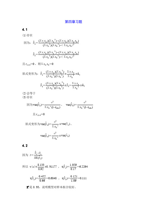
第四章习题4.1(1)存在因为:23223223232322-))(())((-))((ˆ)(ΣΣΣΣΣΣΣ=βi i i i i i i i i i i x x x x x x x y x x y 23223223222233-))(())((-))((ˆ)(ΣΣΣΣΣΣΣ=βi i i i i i i i i i i x x x x x x x y x x y 且032=x x r ,则032=Σi i x x 原式变形为:))(())((ˆ23222322i i i i i x x x x y ΣΣΣΣ=β=222ii i x x y ΣΣ=2αˆ ))(())((ˆ23222233i i i i i x x x x y ΣΣΣΣ=β=2333ˆi i i x x y ΣΣ=β=3αˆ (2)会等于(3)存在因为)r -1()ˆvar(i3i 22222i x Σσ=β, )r -1()ˆvar(i3i 23232i x Σσ=β 且032=x x r原式变形为2222)ˆvar(ix Σσ=β=)ˆvar(2α, 2323)ˆvar(i x Σσ=β=)ˆvar(3α 4.2因为 )ˆ(-ˆ111βββ=SE t 所以 t(c)=92.8133.8=0.91177 , 2294.60.171.059)ˆt(1==β 6848.00.660.452)ˆt(2==β , 111.01.090.121)ˆt(3==β R 2是0.95,说明模型对样本拟合较好。
F检验,F=107.37> F(3,23)=3.03,回归方程显著。
t检验,t统计量分别为0.91177,6.2294,0.6848,0.111,X2,X3对应的t 统计量绝对值均小于t(23)=2.069,X2,X3的系数不显著,可能存在多重共线性。
4.3(1)LnY=-3.111486+1.338533lnGDP-0.421791lnCPI(2)R2是0.988051,修正的R2为0.987055,说明模型对样本拟合较好。
计量经济学第四章部分课后题(庞皓第三版)

计量经济学第四章作业思考题:4.3 多重共线性的典型表现是什么?判断是否存在多重共线性的方法有哪些?答:(1)多重共线性的典型表现:A.模型拟和较好,但偏回归系数几乎都无统计学意义;B.偏回归系数估计值不稳定,方差很大;C.偏回归系数估计值的符号可能与预期不符或与经验相悖,结果难以解释。
(2)具体的判断方法:A.解释变量之间简单相关系数矩阵法;B.方差扩大因子法;C.直观判断法;D.逐步回归的方法。
4.4 针对出现多重共线性的不同情形,能采取的补救措施有哪些?答:(1)根据经验,可以选择剔除变量,增大样本容量,变换模型形式,利用非样本先验信息,截面数据和时间序列数据并用以及变量变换等不同方法。
(2)采取逐步回归方法由由一元模型开始逐步增加解释变量个数,增加的原则是显著提高可决系数,自身显著而与其他变量之间又不产生共线性。
(3)采取岭回归方法来降低多重共线性的程度。
4.9 以下陈述是否正确?请判断并说明理由。
(1)在高度多重共线性的情形中,要评价一个或多个偏回归系数的单个显著性是不可能的。
答:正确。
(2)尽管有完全的多重共线性,OLS估计量仍然是BLUE。
答:错误。
(3)如果有某一辅助回归显示出高的R j2值,则高度共线性的存在肯定是无疑的。
答:正确。
(4)变量的两两高度相关并不表示高度多重共线性。
答:正确。
(5)如果其他条件不变,VIF越高,OLS估计量的方差越大。
答:正确。
(6)如果在多元回归中,根据通常的t检验,全部偏回归系数分别都是统计上不显著的,你就不会得到一个高的R2值。
答:错误。
(7)在Y对X2和X3的回归中,假如X3的值很少变化,这就会使Var(β3)增大,极端的情况下,如果全部X3值都相同,Var(β3) 将是无穷大。
答:正确。
(8)如果分析的目的仅仅是预测,则多重共线性是无害的。
答:错误。
练习题:4.3(1)利用eviews分析得到如下数据:Dependent Variable: LNYMethod: Least SquaresDate: 05/09/16 Time: 12:45Sample: 1985 2011Included observations: 27Variable Coefficient Std. Error t-Statistic Prob.C -3.111486 0.463010 -6.720126 0.0000LNGDP 1.338533 0.088610 15.10582 0.0000LNCPI -0.421791 0.233295 -1.807975 0.0832R-squared 0.988051 Mean dependent var 9.484710Adjusted R-squared 0.987055 S.D. dependent var 1.425517S.E. of regression 0.162189 Akaike info criterion -0.695670Sum squared resid 0.631326 Schwarz criterion -0.551689Log likelihood 12.39155 Hannan-Quinn criter. -0.652857F-statistic 992.2583 Durbin-Watson stat 0.522613Prob(F-statistic) 0.000000由上可知,模型为:lnY=1.338533lnGDP t—0.421791lnCPI t—3.111486(2)A.该模型的可决系数为0.988051,修正可决系数为0.987055,两者都很高。
第四章练习题及参考解答(第四版)计量经济学

第四章练习题及参考解答4.1 假设在模型i i i i u X X Y +++=33221βββ中,32X X 与之间的相关系数为零,有人建议你分别进行如下回归:1221i i i Y X u αα=++ 1332i i i Y X u γγ=++(1) 是否存在3322ˆˆˆˆβγβα==且?为什么? (2) 1ˆβ会等于1ˆα或1ˆγ或者两者的某个线性组合吗? (3) 是否有()()22ˆˆVar Var βα=且()()33ˆˆVar Var βγ=?【练习题4.1参考解答】(1) 存在2233ˆˆˆˆαβγβ==且 。
因为 ()()()()()()()22332322222323ˆi iii ii iiii iy x x y x x x x x x x β-=-∑∑∑∑∑∑∑当23X X 与 之间的相关系数为零时,离差形式的230i ix x =∑有 ()()()()223222222223ˆˆi i ii i iiiy x x y x xx x βα===∑∑∑∑∑∑ 同理有: 33ˆˆγβ= (2)会的。
(3) 存在 ()()()()2233ˆˆˆˆvar var var var βαβγ==且 因为 ()()2222223ˆvar 1ix r σβ=-∑当 230r = 时, ()()()22222222223ˆˆvar var 1iix x r σσβα===-∑∑ 同理,有 ()()33ˆˆvar var βγ=4.2 表4.4给出了1995—2016年中国商品进口额Y 、国生产总值GDP 、居民消费价格指数CPI 的数据。
表4.4 中国商品进口额、国生产总值、居民消费价格指数资料来源:《中国统计年鉴2017》考虑建立模型: i t t t u CPI GDP Y ++=ln ln ln 321βββ+ (1)利用表中数据估计此模型的参数。
(2)你认为数据中有多重共线性吗?(3)进行以下回归:121ln ln t t i Y A A GDP v =++ 122ln ln t t i Y B B CPI v =++ 123ln ln t t i GDP C C CPI v =++ 根据这些回归你能对多重共线性的性质有什么认识?(4)假设经检验数据有多重共线性,但模型中32ˆˆββ和在5%水平上显著,并且F 检验也显著,你对此模型的应用有何建议?【练习题4.2参考解答】建立模型: i t t t u CPI GDP Y ++=ln ln ln 321βββ+ (1)利用表中数据估计此模型的参数。
《计量经济学》第3章、第4章课后题答案

第三、四章习题09国贸1班张继云 1403.31)为分析家庭书刊年消费支出(Y)对家庭月平均收入(X)与户主受教育年数(T)的关系,做如图所示的线形图。
建立多元线性回归模型为Y i=β1+β2X+β3T+μi2) 假定所建立模型中的随机扰动项μi满足各项古典假设,用OLS法估计其参数,得到的回归结果如下。
可用规范形式将参数估计和检验结果写为Y = -50.01638+0.086450X+52.37031T(49.46026)(0.029363)(5.202167)t=(-1.011244)(2.944186)(10.06702)R2=0.951235 F=146.2974 n=183)对回归系数β3的t检验:针对H0:β3=0和H1:β3≠0,由回归结果中还可以看出,估计的回归系数β3的标准误差和t值分别为:SE(β3)= 5.202167, t(β3)= 10.6702。
当α=0.05时,查t分布表得自由度n-3=18-3=15的临界值t0.025(15)=2.131。
因为t(β1)= 10.6702> t0.025(16)=2.131,所以应该拒绝H0:β2=0。
这表明户主受教育年数对家庭书刊年消费支出有显著性影响。
4)所估计的模型的经济意义是当户主受教育年数保持不变时,家庭月平均收入每增加一元时将导致家庭书刊年消费支出增加0.086450元。
而当家庭月平均收入保持不变时,户主受教育年数每增加一年时将导致家庭书刊年消费支出增加52.37031元。
此模型可用于预测将来的家庭书刊年消费支出。
4.31)假定所建立模型中的随机扰动项μi满足各项古典假设,用OLS法估计其参数,得到的回归结果如下。
可用规范形式将参数估计和检验结果写为LnY t = -3.060638+1.056682lnGDP t-1.656536lnCPI t(0.337331)(0.092174) (0.214570)t = (-9.073096) (17.97182) (-4.924656)R2=0.992222 F=1275.739 n=232)数据中有多重共线性,居民消费价格指数的回归系数的符号不能进行合理的经济意义解释,且其简单相关系数呈现正向变动。
- 1、下载文档前请自行甄别文档内容的完整性,平台不提供额外的编辑、内容补充、找答案等附加服务。
- 2、"仅部分预览"的文档,不可在线预览部分如存在完整性等问题,可反馈申请退款(可完整预览的文档不适用该条件!)。
- 3、如文档侵犯您的权益,请联系客服反馈,我们会尽快为您处理(人工客服工作时间:9:00-18:30)。
17CHAPTER 4SOLUTIONS TO PROBLEMS4.2 (i) and (iii) generally cause the t statistics not to have a t distribution under H 0.Homoskedasticity is one of the CLM assumptions. An important omitted variable violates Assumption MLR.3. The CLM assumptions contain no mention of the sample correlations among independent variables, except to rule out the case where the correlation is one.4.3 (i) While the standard error on hrsemp has not changed, the magnitude of the coefficient has increased by half. The t statistic on hrsemp has gone from about –1.47 to –2.21, so now the coefficient is statistically less than zero at the 5% level. (From Table G.2 the 5% critical value with 40 df is –1.684. The 1% critical value is –2.423, so the p -value is between .01 and .05.)(ii) If we add and subtract 2βlog(employ ) from the right-hand-side and collect terms, we havelog(scrap ) = 0β + 1βhrsemp + [2βlog(sales) – 2βlog(employ )] + [2βlog(employ ) + 3βlog(employ )] + u = 0β + 1βhrsemp + 2βlog(sales /employ ) + (2β + 3β)log(employ ) + u ,where the second equality follows from the fact that log(sales /employ ) = log(sales ) – log(employ ). Defining 3θ ≡ 2β + 3β gives the result.(iii) No. We are interested in the coefficient on log(employ ), which has a t statistic of .2, which is very small. Therefore, we conclude that the size of the firm, as measured by employees, does not matter, once we control for training and sales per employee (in a logarithmic functional form).(iv) The null hypothesis in the model from part (ii) is H 0:2β = –1. The t statistic is [–.951 – (–1)]/.37 = (1 – .951)/.37 ≈ .132; this is very small, and we fail to reject whether we specify a one- or two-sided alternative.4.4 (i) In columns (2) and (3), the coefficient on profmarg is actually negative, although its t statistic is only about –1. It appears that, once firm sales and market value have been controlled for, profit margin has no effect on CEO salary.(ii) We use column (3), which controls for the most factors affecting salary. The t statistic on log(mktval ) is about 2.05, which is just significant at the 5% level against a two-sided alternative.18(We can use the standard normal critical value, 1.96.) So log(mktval ) is statistically significant. Because the coefficient is an elasticity, a ceteris paribus 10% increase in market value is predicted to increase salary by 1%. This is not a huge effect, but it is not negligible, either.(iii) These variables are individually significant at low significance levels, with t ceoten ≈ 3.11 and t comten ≈ –2.79. Other factors fixed, another year as CEO with the company increases salary by about 1.71%. On the other hand, another year with the company, but not as CEO, lowers salary by about .92%. This second finding at first seems surprising, but could be related to the “superstar” effect: firms that hire CEOs from outside the company often go after a small pool of highly regarded candidates, and salaries of these people are bid up. More non-CEO years with a company makes it less likely the person was hired as an outside superstar.4.7 (i) .412 ± 1.96(.094), or about .228 to .596.(ii) No, because the value .4 is well inside the 95% CI.(iii) Yes, because 1 is well outside the 95% CI.4.8 (i) With df = 706 – 4 = 702, we use the standard normal critical value (df = ∞ in Table G.2), which is 1.96 for a two-tailed test at the 5% level. Now t educ = −11.13/5.88 ≈ −1.89, so |t educ | = 1.89 < 1.96, and we fail to reject H 0: educ β = 0 at the 5% level. Also, t age ≈ 1.52, so age is also statistically insignificant at the 5% level.(ii) We need to compute the R -squared form of the F statistic for joint significance. But F = [(.113 − .103)/(1 − .113)](702/2) ≈ 3.96. The 5% critical value in the F 2,702 distribution can be obtained from Table G.3b with denominator df = ∞: cv = 3.00. Therefore, educ and age are jointly significant at the 5% level (3.96 > 3.00). In fact, the p -value is about .019, and so educ and age are jointly significant at the 2% level.(iii) Not really. These variables are jointly significant, but including them only changes the coefficient on totwrk from –.151 to –.148.(iv) The standard t and F statistics that we used assume homoskedasticity, in addition to the other CLM assumptions. If there is heteroskedasticity in the equation, the tests are no longer valid.4.11 (i) Holding profmarg fixed, n rdintensΔ = .321 Δlog(sales ) = (.321/100)[100log()sales ⋅Δ] ≈ .00321(%Δsales ). Therefore, if %Δsales = 10, n rdintens Δ ≈ .032, or only about 3/100 of a percentage point. For such a large percentage increase in sales,this seems like a practically small effect.(ii) H 0:1β = 0 versus H 1:1β > 0, where 1β is the population slope on log(sales ). The t statistic is .321/.216 ≈ 1.486. The 5% critical value for a one-tailed test, with df = 32 – 3 = 29, is obtained from Table G.2 as 1.699; so we cannot reject H 0 at the 5% level. But the 10% criticalvalue is 1.311; since the t statistic is above this value, we reject H0 in favor of H1 at the 10% level.(iii) Not really. Its t statistic is only 1.087, which is well below even the 10% critical value for a one-tailed test.1920SOLUTIONS TO COMPUTER EXERCISESC4.1 (i) Holding other factors fixed,111log()(/100)[100log()](/100)(%),voteA expendA expendA expendA βββΔ=Δ=⋅Δ≈Δwhere we use the fact that 100log()expendA ⋅Δ ≈ %expendA Δ. So 1β/100 is the (ceteris paribus) percentage point change in voteA when expendA increases by one percent.(ii) The null hypothesis is H 0: 2β = –1β, which means a z% increase in expenditure by A and a z% increase in expenditure by B leaves voteA unchanged. We can equivalently write H 0: 1β + 2β = 0.(iii) The estimated equation (with standard errors in parentheses below estimates) isn voteA = 45.08 + 6.083 log(expendA ) – 6.615 log(expendB ) + .152 prtystrA(3.93) (0.382) (0.379) (.062) n = 173, R 2 = .793.The coefficient on log(expendA ) is very significant (t statistic ≈ 15.92), as is the coefficient on log(expendB ) (t statistic ≈ –17.45). The estimates imply that a 10% ceteris paribus increase in spending by candidate A increases the predicted share of the vote going to A by about .61percentage points. [Recall that, holding other factors fixed, n voteAΔ≈(6.083/100)%ΔexpendA ).] Similarly, a 10% ceteris paribus increase in spending by B reduces n voteAby about .66 percentage points. These effects certainly cannot be ignored.While the coefficients on log(expendA ) and log(expendB ) are of similar magnitudes (andopposite in sign, as we expect), we do not have the standard error of 1ˆβ + 2ˆβ, which is what we would need to test the hypothesis from part (ii).(iv) Write 1θ = 1β +2β, or 1β = 1θ– 2β. Plugging this into the original equation, and rearranging, givesn voteA = 0β + 1θlog(expendA ) + 2β[log(expendB ) – log(expendA )] +3βprtystrA + u ,When we estimate this equation we obtain 1θ≈ –.532 and se( 1θ)≈ .533. The t statistic for the hypothesis in part (ii) is –.532/.533 ≈ –1. Therefore, we fail to reject H 0: 2β = –1β.21C4.3 (i) The estimated model isn log()price = 11.67 + .000379 sqrft + .0289 bdrms (0.10) (.000043) (.0296)n = 88, R 2 = .588.Therefore, 1ˆθ= 150(.000379) + .0289 = .0858, which means that an additional 150 square foot bedroom increases the predicted price by about 8.6%.(ii) 2β= 1θ – 1501β, and solog(price ) = 0β+ 1βsqrft + (1θ – 1501β)bdrms + u= 0β+ 1β(sqrft – 150 bdrms ) + 1θbdrms + u .(iii) From part (ii), we run the regressionlog(price ) on (sqrft – 150 bdrms ), bdrms ,and obtain the standard error on bdrms . We already know that 1ˆθ= .0858; now we also getse(1ˆθ) = .0268. The 95% confidence interval reported by my software package is .0326 to .1390(or about 3.3% to 13.9%).C4.5 (i) If we drop rbisyr the estimated equation becomesn log()salary = 11.02 + .0677 years + .0158 gamesyr (0.27) (.0121) (.0016)+ .0014 bavg + .0359 hrunsyr (.0011) (.0072)n = 353, R 2= .625.Now hrunsyr is very statistically significant (t statistic ≈ 4.99), and its coefficient has increased by about two and one-half times.(ii) The equation with runsyr , fldperc , and sbasesyr added is22n log()salary = 10.41 + .0700 years + .0079 gamesyr(2.00) (.0120) (.0027)+ .00053 bavg + .0232 hrunsyr (.00110) (.0086)+ .0174 runsyr + .0010 fldperc – .0064 sbasesyr (.0051) (.0020) (.0052) n = 353, R 2 = .639.Of the three additional independent variables, only runsyr is statistically significant (t statistic = .0174/.0051 ≈ 3.41). The estimate implies that one more run per year, other factors fixed,increases predicted salary by about 1.74%, a substantial increase. The stolen bases variable even has the “wrong” sign with a t statistic of about –1.23, while fldperc has a t statistic of only .5. Most major league baseball players are pretty good fielders; in fact, the smallest fldperc is 800 (which means .800). With relatively little variation in fldperc , it is perhaps not surprising that its effect is hard to estimate.(iii) From their t statistics, bavg , fldperc , and sbasesyr are individually insignificant. The F statistic for their joint significance (with 3 and 345 df ) is about .69 with p -value ≈ .56. Therefore, these variables are jointly very insignificant.C4.7 (i) The minimum value is 0, the maximum is 99, and the average is about 56.16. (ii) When phsrank is added to (4.26), we get the following:n log() wage = 1.459 − .0093 jc + .0755 totcoll + .0049 exper + .00030 phsrank (0.024) (.0070) (.0026) (.0002) (.00024)n = 6,763, R 2 = .223So phsrank has a t statistic equal to only 1.25; it is not statistically significant. If we increase phsrank by 10, log(wage ) is predicted to increase by (.0003)10 = .003. This implies a .3% increase in wage , which seems a modest increase given a 10 percentage point increase in phsrank . (However, the sample standard deviation of phsrank is about 24.)(iii) Adding phsrank makes the t statistic on jc even smaller in absolute value, about 1.33, but the coefficient magnitude is similar to (4.26). Therefore, the base point remains unchanged: the return to a junior college is estimated to be somewhat smaller, but the difference is not significant and standard significant levels.(iv) The variable id is just a worker identification number, which should be randomly assigned (at least roughly). Therefore, id should not be correlated with any variable in the regression equation. It should be insignificant when added to (4.17) or (4.26). In fact, its t statistic is about .54.23C4.9 (i) The results from the OLS regression, with standard errors in parentheses, aren log() psoda =−1.46 + .073 prpblck + .137 log(income ) + .380 prppov (0.29) (.031) (.027) (.133)n = 401, R 2 = .087The p -value for testing H 0: 10β= against the two-sided alternative is about .018, so that we reject H 0 at the 5% level but not at the 1% level.(ii) The correlation is about −.84, indicating a strong degree of multicollinearity. Yet eachcoefficient is very statistically significant: the t statistic for log()ˆincome β is about 5.1 and that forˆprppovβ is about 2.86 (two-sided p -value = .004).(iii) The OLS regression results when log(hseval ) is added aren log() psoda =−.84 + .098 prpblck − .053 log(income ) (.29) (.029) (.038) + .052 prppov + .121 log(hseval ) (.134) (.018)n = 401, R 2 = .184The coefficient on log(hseval ) is an elasticity: a one percent increase in housing value, holding the other variables fixed, increases the predicted price by about .12 percent. The two-sided p -value is zero to three decimal places.(iv) Adding log(hseval ) makes log(income ) and prppov individually insignificant (at even the 15% significance level against a two-sided alternative for log(income ), and prppov is does not have a t statistic even close to one in absolute value). Nevertheless, they are jointly significant at the 5% level because the outcome of the F 2,396 statistic is about 3.52 with p -value = .030. All of the control variables – log(income ), prppov , and log(hseval ) – are highly correlated, so it is not surprising that some are individually insignificant.(v) Because the regression in (iii) contains the most controls, log(hseval ) is individually significant, and log(income ) and prppov are jointly significant, (iii) seems the most reliable. It holds fixed three measure of income and affluence. Therefore, a reasonable estimate is that if the proportion of blacks increases by .10, psoda is estimated to increase by 1%, other factors held fixed.。