外文文献资料(Canny 算子)
canny sobel算子
基于sobel 、canny 的边缘检测实现一.实验原理Sobel 的原理:索贝尔算子(Sobel operator )是图像处理中的算子之一,主要用作边缘检测。
在技术上,它是一离散性差分算子,用来运算图像亮度函数的梯度之近似值。
在图像的任何一点使用此算子,将会产生对应的梯度矢量或是其法矢量.该算子包含两组3x3的矩阵,分别为横向及纵向,将之与图像作平面卷积,即可分别得出横向及纵向的亮度差分近似值。
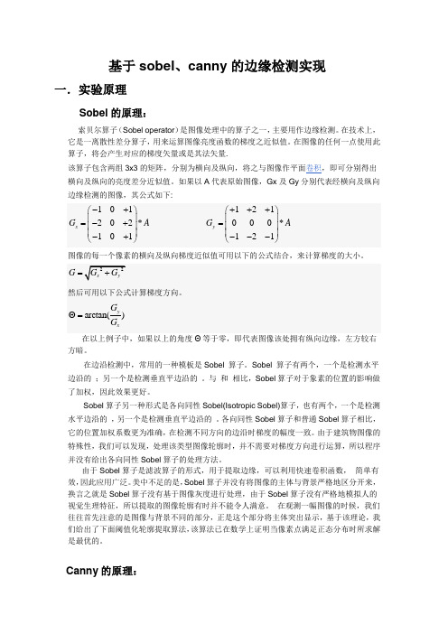
如果以A 代表原始图像,Gx 及Gy 分别代表经横向及纵向边缘检测的图像,其公式如下:101202*101x G A -+⎛⎫ ⎪=-+ ⎪ ⎪-+⎝⎭ 121000*121y G A +++⎛⎫ ⎪= ⎪ ⎪---⎝⎭图像的每一个像素的横向及纵向梯度近似值可用以下的公式结合,来计算梯度的大小。
在以上例子中,如果以上的角度Θ等于零,即代表图像该处拥有纵向边缘,左方较右方暗。
在边沿检测中,常用的一种模板是Sobel 算子。
Sobel 算子有两个,一个是检测水平边沿的 ;另一个是检测垂直平边沿的 。
与 和 相比,Sobel 算子对于象素的位置的影响做了加权,因此效果更好。
Sobel 算子另一种形式是各向同性Sobel(Isotropic Sobel)算子,也有两个,一个是检测水平边沿的 ,另一个是检测垂直平边沿的 。
各向同性Sobel 算子和普通Sobel 算子相比,它的位置加权系数更为准确,在检测不同方向的边沿时梯度的幅度一致。
由于建筑物图像的特殊性,我们可以发现,处理该类型图像轮廓时,并不需要对梯度方向进行运算,所以程序并没有给出各向同性Sobel 算子的处理方法。
由于Sobel 算子是滤波算子的形式,用于提取边缘,可以利用快速卷积函数, 简单有效,因此应用广泛。
美中不足的是,Sobel 算子并没有将图像的主体与背景严格地区分开来,换言之就是Sobel 算子没有基于图像灰度进行处理,由于Sobel 算子没有严格地模拟人的视觉生理特征,所以提取的图像轮廓有时并不能令人满意。
Canny算子
1、边缘检测原理及步骤在之前的博文中,作者从一维函数的跃变检测开始,循序渐进的对二维图像边缘检测的基本原理进行了通俗化的描述。
结论是:实现图像的边缘检测,就是要用离散化梯度逼近函数根据二维灰度矩阵梯度向量来寻找图像灰度矩阵的灰度跃变位置,然后在图像中将这些位置的点连起来就构成了所谓的图像边缘(图像边缘在这里是一个统称,包括了二维图像上的边缘、角点、纹理等基元图)。
在实际情况中理想的灰度阶跃及其线条边缘图像是很少见到的,同时大多数的传感器件具有低频滤波特性,这样会使得阶跃边缘变为斜坡性边缘,看起来其中的强度变化不是瞬间的,而是跨越了一定的距离。
这就使得在边缘检测中首先要进行的工作是滤波。
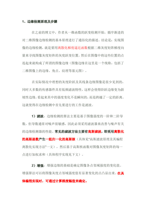
1)滤波:边缘检测的算法主要是基于图像强度的一阶和二阶导数,但导数通常对噪声很敏感,因此必须采用滤波器来改善与噪声有关的边缘检测器的性能。
常见的滤波方法主要有高斯滤波,即采用离散化的高斯函数产生一组归一化的高斯核(具体见“高斯滤波原理及其编程离散化实现方法”一文),然后基于高斯核函数对图像灰度矩阵的每一点进行加权求和(具体程序实现见下文)。
2)增强:增强边缘的基础是确定图像各点邻域强度的变化值。
增强算法可以将图像灰度点邻域强度值有显著变化的点凸显出来。
在具体编程实现时,可通过计算梯度幅值来确定。
3)检测:经过增强的图像,往往邻域中有很多点的梯度值比较大,而在特定的应用中,这些点并不是我们要找的边缘点,所以应该采用某种方法来对这些点进行取舍。
实际工程中,常用的方法是通过阈值化方法来检测。
2、Canny边缘检测算法原理JohnCanny于1986年提出Canny算子,它与Marr(LoG)边缘检测方法类似,也属于是先平滑后求导数的方法。
本节对根据上述的边缘检测过程对Canny检测算法的原理进行介绍。
2.1 对原始图像进行灰度化Canny算法通常处理的图像为灰度图,因此如果摄像机获取的是彩色图像,那首先就得进行灰度化。
对一幅彩色图进行灰度化,就是根据图像各个通道的采样值进行加权平均。
基于改进的Canny算子图像信息提取算法研究
( 东 松 山职 业 技 术 学 院 计 算 机 系 , 东 韶关 5 2 2 ) 广 广 1 16
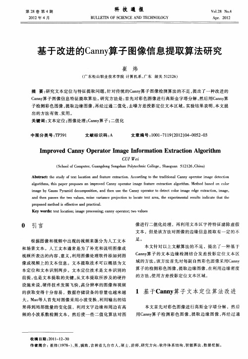
摘 要: 研究文 本定位 与特征提取 问题 。 针对传统 的C n y an算子 图像检测算法 的不足 , 提出了一种改进的 C ny a n算子 图像信息特征提取算法。 研究方法是 : 首先对彩色图像进行高斯金字塔分解 , 然后用C n y an 算
用 C n y 子 检 测 彩 色 图像 , 取 边 缘 图 像 , 经 过 通 an 算 提 再
1 基 于C n y a n 算子 文本 定 位 算 法 改进
频 的小波系数检测文本 ,然后使一些二值化算法对 图
收 稿 日期 : 0 1 1 — 0 2 1- 2 3
前 提 , 是 文 本 提 取 的关 键 , 文 本 提 取所 涉 及 的 硬 件 也 从
算子 的检测彩色 图像 , 提取边缘图像 , 利用边 缘密度 在
的方 法 , 用 方 差 投 影 定 位 文 本 区域 。 使
设 施来说 , 硬件技术发展飞快 , 高分辨率的图像和视频 的获取变得 十分容易 ,数据存储设备的容量也越来越 大。 o Ma等人首先对 图像采用小波变换 , 利用输 出的结 果得到局部能量的变化值 ,利用文字边缘和周边有高 本文首先对彩色 图像进行高斯金字塔分解 ,然后
I p o e n y Op r t rI g n o ma i n Ex r ci n Alo i m m r v d Ca n e a o ma e I f r t ta t g rt o o h
canny算子边缘检测原理

canny算子边缘检测原理
Canny算子是一种常用的边缘检测算法,其原理如下:
1. 高斯滤波:首先对图像进行高斯滤波,以减少噪声的影响。
高斯滤波是利用高斯函数对图像进行平滑操作,可以抑制高频噪声。
2. 计算梯度幅值和方向:对平滑后的图像进行梯度计算,通过计算像素点的梯度幅值和方向,可以找到图像中的边缘。
常用的梯度算子包括Sobel算子和Prewitt算子。
3. 非极大值抑制:在梯度图像中,对于每个像素点,通过比较其梯度方向上的两个相邻像素点的梯度幅值,将梯度幅值取最大值的点保留下来,其他点置为0。
这样可以剔除非边缘的像素。
4. 双阈值处理:将梯度幅值图像中的像素分为强边缘、弱边缘和非边缘三类。
设置两个阈值:高阈值和低阈值。
如果某个像素的梯度幅值大于高阈值,则将其标记为强边缘。
如果某个像素的梯度幅值小于低阈值,则将其剔除。
对于梯度幅值介于低阈值和高阈值之间的像素,如果其与某个强边缘像素相连,则将其标记为强边缘,否则将其标记为弱边缘。
5. 边缘连接:通过将强边缘和与其相连的弱边缘进行连接,找到完整的边缘。
这里通常使用8连通或4连通算法来判断两个像素是否相连。
通过以上步骤,Canny算子可以得到图像中的边缘信息,并且相对其他算法能够更好地抑制噪声和保持边缘的连续性。
边缘分割(Canny算子)
边缘分割(Canny算⼦)最近有⽤到Canny算⼦做边缘检测。
回顾⼀下Canny算⼦的基本原理:总的来说,图像的边缘检测必须满⾜两个步骤(1)有效的抑制噪声,使⽤⾼斯算⼦对图像进⾏平滑;(2)尽量精确的确定边缘的位置;Canny算⼦的边缘检测可以分为三个步骤:Step 1: ⾼斯平滑函数。
⽬的是为了平滑以消除噪声;Step 2:⼀阶差分卷积模板。
⽬的是为了达到边缘增强。
该步骤有点类似于与两个⽅向模板进⾏卷积运算。
这两个⽅向模板为(a)和(b)所⽰:左图体现的是在X⽅向上的差异,右图体现的是在y⽅向上的差异。
同时获得梯度幅值的⼤⼩以及⽅向⾓。
通过该步,获得在边缘位置处特征被加强的图像。
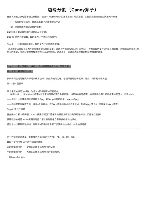
Step 3:⾮极⼤值抑制(NMS)。
⽬的是保留梯度⽅向上的最⼤值。
这⼀步是⽐较关键的⼀点:仅仅得到全局的梯度并不⾜以确定边缘,因此为确定边缘,必须保留局部梯度最⼤的点,⽽抑制⾮极⼤值图2⾮极⼤值抑制四个扇区的标号为0到3,对应3*3邻域的四种可能组合。
在每⼀点上,邻域的中⼼象素M与沿着梯度线的两个象素相⽐。
如果M的梯度值不⽐沿梯度线的两个相邻象素梯度值⼤,则令M=0。
——假设上⼀步骤得到的梯度图为G(x,y);对G(x,y)进⾏初始化:N(x,y)=G(x,y)——在梯度和反梯度⽅向上各找n个像素点。
若G(x,y)不是这些点中的最⼤点,则将N(x,y)置为0,否则保持N(x,y)不变。
Step4: 双线性阈值⾸先是⼀个较⼤的阈值:Nmax.使⽤该阈值⼆值化后的图像含有较少的假的边缘点,但是端点较多!使⽤较⼩的阈值:Nmin,使⽤该阈值⼆值化后的图像含有较多的假的边缘点;通过上⼀步获取的边缘点,判断其8邻域内有⽆第⼆步获得的边缘点,然后进⾏连接!另⼀种简单的⽅法是,把梯度⽅向简化为4个⽅向:『0,45,90,135』最后⼀步为对N(x,y)进⾏阈值化处理:⼤的阈值会得到——少量的边缘点以及众多的空隙⼩的阈值会得到——⼤量的边缘点以及众多的错误检测。
canny算子
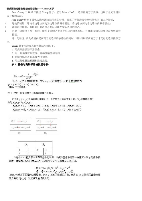
经典图像边缘检测(综合法思想)——Canny算子John Canny于1986年提出Canny算子,它与Marr(LoG)边缘检测方法类似,也属于是先平滑后求导数的方法。
John Canny研究了最优边缘检测方法所需的特性,给出了评价边缘检测性能优劣的三个指标:l好的信噪比,即将非边缘点判定为边缘点的概率要低,将边缘点判为非边缘点的概率要低;l高的定位性能,即检测出的边缘点要尽可能在实际边缘的中心;l对单一边缘仅有唯一响应,即单个边缘产生多个响应的概率要低,并且虚假响应边缘应该得到最大抑制。
用一句话说,就是希望在提高对景物边缘的敏感性的同时,可以抑制噪声的方法才是好的边缘提取方法。
Canny算子求边缘点具体算法步骤如下:1. 用高斯滤波器平滑图像.2. 用一阶偏导有限差分计算梯度幅值和方向.3. 对梯度幅值进行非极大值抑制.4. 用双阈值算法检测和连接边缘.步1. 图像与高斯平滑滤波器卷积:步3. 对梯度幅值进行非极大值抑制(non_maxima suppression,NMS):仅仅得到全局的梯度并不足以确定边缘,因此为确定边缘,必须保留局部梯度最大的点,而抑制非极大值。
解决方法:利用梯度的方向:步4. 用双阈值算法检测和连接边缘:对非极大值抑制图像作用两个阈值th1和th2,两者关系th1=0.4th2。
我们把梯度值小于th1的像素的灰度值设为0,得到图像1。
然后把梯度值小于th2的像素的灰度值设为0,得到图像2。
由于图像2的阈值较高,去除大部分噪音,但同时也损失了有用的边缘信息。
而图像1的阈值较低,保留了较多的信息,我们可以以图像2为基础,以图像1为补充来连结图像的边缘。
链接边缘的具体步骤如下:对图像2进行扫描,当遇到一个非零灰度的像素p(x,y)时,跟踪以p(x,y)为开始点的轮廓线,直到轮廓线的终点q(x,y)。
考察图像1中与图像2中q(x,y)点位置对应的点s(x,y)的8邻近区域。
Canny算子在织物防水性能自动识别中的应用
点 , 据 目标边 缘 点 的灰 度 梯 度 比非 边 缘 点灰 度 梯 根 度大 的特 点 , 取 适 当阈 值 来 判 断 边缘 点 , 提 选 是
统 的方 法 主要 依 赖人工 检测 , 劳动 强度 大 , 易受心 容
理、 生理 和环 境等 因素 的影 响 , 导致 检 测 误差 大 , 一
ZHU i i g, Z Gu y n HANG ii Ru l n
( hj n c— eh U i rt Z ea gS lTc nv sy,Ha gh u,Z 4a g 3 0 1  ̄ ei n zo h in 10 8,C ia) hn
Ab t a t T i a e rpoe n lo t m f a tmai ee to f fb c waep o f p roma c u i g s r c h s p p rp o s d a ag r h o u o tc d tcin o a r tr r o e r n e sn i i f i g r c s n o u e e h oo y a c r i g t h r p riso tfb c a d rlt d sa d r s.Fis , ma ep o e sa d c mp trtc n lg c od n o t e p o ete fwe a r n eae tn ad i rt t e i g ft ewe a rc wa n lz d,a d t e h ma e o h tfb sa ay e i n h n,Ca n p rtra d Otu ag rt n y o eao n s lo hm r s d i ee t n i wee u e n d tci o o h a rc e g ft ef i d e,i efa a tv n s n t e a tmai ee to ffb c wae ro roma c sr aie b t s l-d p ie e si h uo t d tcin o r tr o f f r n e wa e l d s c ai p pe z a d isp o e sn ae a d c oc fp r mee swee i r v d.F rh r r n t r c si gr t n h ie o aa t r r mp o e u emoe,mo h lg c la t mei rc s t p r oo ia r h t p o e s i c wa s d t e h ls d e g ft e w tfb c. su e o g tt e coe d e o h e a r i K e r s Ca n p rtr u o tc d tci n;fb c;wae ro e o a c y wo d n y o e ao ;a tmai ee t o ar i tr o fp r r n e p f m
基于canny算子的边缘检测算法应用研究
基于canny算子的边缘检测算法应用研究作者:陈蒙来源:《电子技术与软件工程》2013年第23期摘要:边缘检测技术是图像处理过程的重要一环,本文主要研究基于canny算则的边缘检测算法中的抑制噪声、寻找亮度梯度、非极大值抑制、边缘的确定和连接等四个过程,并逐个分析其实现过程及作用。
【关键词】边缘检测高斯平滑1 引言随着图像处理技术的发展与广泛应用,现在社会中图像处理的应用领域越来越广泛,如三维重建,医学诊断,图像识别等等。
而图像处理过程中,最重要的一项预处理技术即为边缘检测技术。
图像的边缘是图像特征识别中的重要组成部分。
我们一般认为边缘是图像中周围像素有不连续变化或屋脊变化的像素的集合。
在一幅图像中,边缘特征所表达的信息量在整张图片的特征信息中占有主导地位,对图像特征的识别、分析十分重要。
边缘信息主要从像素值幅度和走向两个方面来表示。
一般来说,沿着边缘走向的像素点灰度值呈连续性变化特征,而垂直于边缘走向的像素点灰度值则呈跳跃性或阶跃性变化特征。
边缘检测技术即为通过一定的算法将图像中的边缘尽可能真实地提取或表示出来的技术。
边缘检测技术发展到目前已有很多类提取算法,但主要的计算原则就借助于类似高斯平滑、傅里叶变换等的数学函数与图像的灰度矩阵进行卷积计算,从而得到横、纵两个方向上的梯度图像和模图像,然后根据梯度方向来进行模的极大值提取,获得需要的图像特征边缘。
本文主要研究的是以canny算子为检测手段的边缘检测算法。
2 canny边缘检测算法任何一个边缘检测算法的原则都是真实、详尽地标识出原图像的实际边缘,同时又尽可能避免图像中的噪点、伪边缘等噪声的干扰,找到一个最优的图像边缘。
Canny边缘检测算法也是如此,一般由抑制噪声、寻找梯度亮度、非极大值抑制、确定和连接边缘这四步完成的。
2.1 1抑制噪声任何图像在进行边缘检测之前,都要进行抑制噪声的预处理。
它是所有图像处理过程的第一步。
图像的噪声主要有椒盐噪声和高斯噪声两种,而绝大部分图形的干扰噪声属于高斯噪声,因此canny算法的第一步采用的是运用二维高斯平滑模板与原图像数据进行卷积计算,而得到抑制噪声后的待处理图像。
- 1、下载文档前请自行甄别文档内容的完整性,平台不提供额外的编辑、内容补充、找答案等附加服务。
- 2、"仅部分预览"的文档,不可在线预览部分如存在完整性等问题,可反馈申请退款(可完整预览的文档不适用该条件!)。
- 3、如文档侵犯您的权益,请联系客服反馈,我们会尽快为您处理(人工客服工作时间:9:00-18:30)。
外文文献资料Canny edge detector1.Canny edge detector IntroductionThe Canny edge detection operator was developed by John F. Canny in 1986 and uses a multi-stage algorithm to detect a wide range of edges in images. Most importantly, Canny also produced a computational theory of edge detection explaining why the technique works.2. Development of the Canny algorithmCanny's aim was to discover the optimal edge detection algorithm. In this situation, an "optimal" edge detector means:●good detection – the algorithm should mark as many real edges in the imageas possible.●good localization – edges marked should be as close as possible to the edgein the real image.●minimal response – a given edge in the image should only be marked once,and where possible, image noise should not create false edges.To satisfy these requirements Canny used the calculus of variations – a technique which finds the function which optimizes a given functional. Theoptimal function in Canny's detector is described by the sum of four exponential terms, but can be approximated by the first derivative of a Gaussian.3. Stages of the Canny algorithm3.1 Noise reductionThe Canny edge detector uses a filter based on the first derivative of a Gaussian, because it is susceptible to noise present on raw unprocessed image data, so to begin with, the raw image is convolved with a Gaussian filter. The result is a slightly blurred version of the original which is not affected by a single noisy pixel to any significant degree.3.2 Finding the intensity gradient of the imageAn edge in an image may point in a variety of directions, so the Canny algorithm uses four filters to detect horizontal, vertical and diagonal edges in the blurred image. The edge detection operator (Roberts, Prewitt, Sobel for example) returns a value for the first derivative in the horizontal direction (Gy) and the vertical direction (Gx). From this the edge gradient and direction can be determined.3.3 Tracing edges through the image and hysteresis thresholdingIntensity gradients which are large are more likely to correspond to edges than if they are small. It is in most cases impossible to specify a threshold at which agiven intensity gradient switches from corresponding to an edge into not doing so. Therefore Canny uses thresholding with hysteresis.Thresholding with hysteresis requires two thresholds – high and low. Making the assumption that important edges should be along continuous curves in theimage allows us to follow a faint section of a given line and to discard a few noisy pixels that do not constitute a line but have produced large gradients. Therefore we begin by applying a high threshold. This marks out the edges we can be fairly sure are genuine. Starting from these, using the directional information derived earlier, edges can be traced through the image. While tracing an edge, we apply the lower threshold, allowing us to trace faint sections of edges as long as we find a starting point.Once this process is complete we have a binary image where each pixel ismarked as either an edge pixel or a non-edge pixel. From complementary output from the edge tracing step, the binary edge map obtained in this way can also be treated as a set of edge curves, which after further processing can be represented as polygons in the image domain.Differential geometric formulation of the Canny edge detector :0222=++yy y xy y x xx x L L L L L L L (3-1)A more refined approach to obtain edges with sub-pixel accuracy is by using the approach of differential edge detection, where the requirement ofnon-maximum suppression is formulated in terms of second- and third-orderderivatives computed from a scale-space representation (Lindeberg 1998) – see the article on edge detection for a detailed description.Variational-geometric formulation of the Haralick-Canny edge detector :0333223<+++yyy y xyy y x xxy y x xxx x L L L L L L L L L L (3-2)A variational explanation for the main ingredient of the Canny edge detector, that is, finding the zero crossings of the 2nd derivative along the gradient direction, was shown to be the result of minimizing a Kronrod-Minkowski functional while maximizing the integral over the alignment of the edge with the gradient field(Kimmel and Bruckstein 2003) see article on regularized Laplacian zero crossings and other optimal edge integrators for a detailed description.4 ParametersThe Canny algorithm contains a number of adjustable parameters, which can affect the computation time and effectiveness of the algorithm.The size of the Gaussian filter: the smoothing filter used in the first stagedirectly affects the results of the Canny algorithm. Smaller filters cause less blurring, and allow detection of small, sharp lines. A larger filter causesmore blurring, smearing out the value of a given pixel over a larger area of the image. Larger blurring radii are more useful for detecting larger,smoother edges – for instance, the edge of a rainbow.Thresholds: the use of two thresholds with hysteresis allows more flexibility than in a single-threshold approach, but general problems of thresholdingapproaches still apply. A threshold set too high can miss importantinformation. On the other hand, a threshold set too low will falsely identifyirrelevant information (such as noise) as important. It is difficult to give ageneric threshold that works well on all images. No tried and testedapproach to this problem yet exists.5 ConclusionThe Canny algorithm is adaptable to various environments. Its parameters allow it to be tailored to recognition of edges of differing characteristics depending on the particular requirements of a given implementation. In Canny's original paper, the derivation of the optimal filter led to a Finite Impulse Response filter, which can be slow to compute in the spatial domain if the amount of smoothing required is important (the filter will have a large spatial support in that case). For this reason, it is often suggested to use Rachid Deriche's Infinite Impulse Response form of Canny's filter (the Canny-Deriche detector), which is recursive, and which can be computed in a short, fixed amount of time for any desired amount of smoothing. The second form is suitable for real time implementations in FPGAs or DSPs, or very fast embedded PCs. In this context, however, the regular recursive implementation of the Canny operator does not give a good approximation of rotational symmetry and therefore gives a bias towards horizontal and vertical edges.中文翻译稿Canny算子1 Canny算子简介Canny 边缘检测算子是John F. Canny于1986 年开发出来的一个多级边缘检测算法。