matlab 统计工具箱函数
MATLAB中的统计分析工具箱使用技巧

MATLAB中的统计分析工具箱使用技巧引言:统计分析是一门广泛应用于各个领域的学科,它帮助我们理解和解释现实世界中的数据。
MATLAB作为一种强大的科学计算软件,提供了丰富的统计分析工具箱,可以帮助我们在数据处理和分析中取得更好的结果。
本文将介绍一些MATLAB中的统计分析工具箱使用技巧,希望可以为读者带来一些启发和帮助。
一、数据的导入与导出在进行统计分析之前,首先需要将数据导入MATLAB中。
MATLAB提供了多种数据导入方式,包括从文本文件、Excel表格和数据库中导入数据等。
其中,从文本文件导入数据是最常用的方法之一。
可以使用readtable函数将文本文件中的数据读入到MATLAB的数据框中,方便后续的操作和分析。
对于数据的导出,MATLAB也提供了相应的函数,例如writetable函数可以将数据框中的数据写入到文本文件中。
二、数据的预处理在进行统计分析之前,通常需要对数据进行预处理。
预处理包括数据清洗、缺失值处理、异常值处理和数据变换等步骤。
MATLAB提供了一系列函数和工具箱来方便进行数据的预处理。
例如,可以使用ismissing函数判断数据中是否存在缺失值,使用fillmissing函数对缺失值进行填充。
另外,MATLAB还提供了一些常用的数据变换函数,例如log、sqrt、zscore等,可以帮助我们将数据转化为正态分布或者标准化。
三、常用的统计分析方法1. 描述统计分析描述统计分析是对数据进行基本的统计描述,包括计算均值、中位数、标准差、百分位数等。
MATLAB提供了一系列函数来进行描述统计分析,例如mean、median、std等。
这些函数可以帮助我们快速计算和分析数据的基本统计指标。
2. 假设检验假设检验是统计分析中常用的方法之一,用于根据样本数据来推断总体的性质。
MATLAB提供了多种假设检验的函数,例如ttest、anova1、chi2test等。
这些函数可以帮助我们进行双样本或多样本的方差分析、配对样本的t检验、独立样本的t检验等。
matlab统计工具箱函数
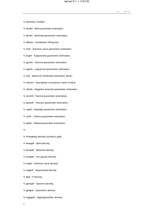
v1.0可编写可改正%Statistics Toolbox%betafit - Beta parameter estimation.%binofit - Binomial parameter estimation.%dfittool - Distribution fitting tool.%evfit - Extreme value parameter estimation.%expfit - Exponential parameter estimation.%gamfit - Gamma parameter estimation.%lognfit - Lognormal parameter estimation.%mle - Maximum likelihood estimation (MLE).%mlecov - Asymptotic covariance matrix of MLE.%nbinfit - Negative binomial parameter estimation.%normfit - Normal parameter estimation.%poissfit - Poisson parameter estimation.%raylfit - Rayleigh parameter estimation.%unifit - Uniform parameter estimation.%wblfit - Weibull parameter estimation.%%Probability density functions (pdf).%betapdf - Beta density.%binopdf - Binomial density.%chi2pdf - Chi square density.%evpdf - Extreme value density.%exppdf - Exponential density.%fpdf - F density.%gampdf - Gamma density.%geopdf - Geometric density.%hygepdf - Hypergeometric density.%lognpdf - Lognormal density.%mvnpdf - Multivariate normal density.%nbinpdf - Negative binomial density.%ncfpdf - Noncentral F density.%nctpdf - Noncentral t density.%ncx2pdf - Noncentral Chi-square density.%normpdf - Normal (Gaussian) density.%pdf - Density function for a specified distribution.%poisspdf - Poisson density.%raylpdf - Rayleigh density.%tpdf - T density.%unidpdf - Discrete uniform density.%unifpdf - Uniform density.%wblpdf - Weibull density.%%Cumulative Distribution functions (cdf).%betacdf - Beta cdf.%binocdf - Binomial cdf.%cdf - Specified cumulative distribution function.%chi2cdf - Chi square cdf.%ecdf - Empirical cdf (Kaplan-Meier estimate).%evcdf - Extreme value cumulative distribution function. %expcdf - Exponential cdf.%fcdf - F cdf.%gamcdf - Gamma cdf.%geocdf - Geometric cdf.%hygecdf - Hypergeometric cdf.%logncdf - Lognormal cdf.%nbincdf - Negative binomial cdf.%ncfcdf - Noncentral F cdf.%nctcdf - Noncentral t cdf.%ncx2cdf - Noncentral Chi-square cdf.%normcdf - Normal (Gaussian) cdf.%poisscdf - Poisson cdf.%raylcdf - Rayleigh cdf.%tcdf - T cdf.%unidcdf - Discrete uniform cdf.%unifcdf - Uniform cdf.%wblcdf - Weibull cdf.%%Critical Values of Distribution functions.%betainv - Beta inverse cumulative distribution function.%binoinv - Binomial inverse cumulative distribution function.%chi2inv - Chi square inverse cumulative distribution function.%evinv - Extreme value inverse cumulative distribution function.%expinv - Exponential inverse cumulative distribution function.%finv - F inverse cumulative distribution function.%gaminv - Gamma inverse cumulative distribution function.%geoinv - Geometric inverse cumulative distribution function.%hygeinv - Hypergeometric inverse cumulative distribution function. %icdf - Specified inverse cdf.%logninv - Lognormal inverse cumulative distribution function.%nbininv - Negative binomial inverse distribution function.%ncfinv - Noncentral F inverse cumulative distribution function.%nctinv - Noncentral t inverse cumulative distribution function.%ncx2inv - Noncentral Chi-square inverse distribution function.%norminv - Normal (Gaussian) inverse cumulative distribution function. %poissinv - Poisson inverse cumulative distribution function.%raylinv - Rayleigh inverse cumulative distribution function.%tinv - T inverse cumulative distribution function.%unidinv - Discrete uniform inverse cumulative distribution function.%unifinv - Uniform inverse cumulative distribution function.%wblinv - Weibull inverse cumulative distribution function.%%Random Number Generators.%betarnd - Beta random numbers.%binornd - Binomial random numbers.%chi2rnd - Chi square random numbers.%evrnd - Extreme value random numbers.%exprnd - Exponential random numbers.%frnd - F random numbers.%gamrnd - Gamma random numbers.%geornd - Geometric random numbers.%hygernd - Hypergeometric random numbers.%iwishrnd - Inverse Wishart random matrix.%lognrnd - Lognormal random numbers.%mvnrnd - Multivariate normal random numbers.%mvtrnd - Multivariate t random numbers.%nbinrnd - Negative binomial random numbers.%ncfrnd - Noncentral F random numbers.%nctrnd - Noncentral t random numbers.%normrnd - Normal (Gaussian) random numbers.%poissrnd - Poisson random numbers.%randg - Gamma random numbers (unit scale).%random - Random numbers from specified distribution. %randsample - Random sample from finite population. %raylrnd - Rayleigh random numbers.%trnd - T random numbers.%unidrnd - Discrete uniform random numbers.%unifrnd - Uniform random numbers.%wblrnd - Weibull random numbers.%wishrnd - Wishart random matrix.%%Statistics.%betastat - Beta mean and variance.%binostat - Binomial mean and variance.%chi2stat - Chi square mean and variance.%evstat - Extreme value mean and variance.%expstat - Exponential mean and variance.%fstat - F mean and variance.%gamstat - Gamma mean and variance.%geostat - Geometric mean and variance.%hygestat - Hypergeometric mean and variance.%lognstat - Lognormal mean and variance.%nbinstat - Negative binomial mean and variance.%ncfstat - Noncentral F mean and variance.%nctstat - Noncentral t mean and variance.%normstat - Normal (Gaussian) mean and variance.%poisstat - Poisson mean and variance.%raylstat - Rayleigh mean and variance.%tstat - T mean and variance.%unidstat - Discrete uniform mean and variance.%unifstat - Uniform mean and variance.%wblstat - Weibull mean and variance.%%Likelihood functions.%betalike - Negative beta log-likelihood.%evlike - Negative extreme value log-likelihood.%explike - Negative exponential log-likelihood.%gamlike - Negative gamma log-likelihood.%lognlike - Negative lognormal log-likelihood.%nbinlike - Negative likelihood for negative binomial distribution. %normlike - Negative normal likelihood.%wbllike - Negative Weibull log-likelihood.%%Descriptive Statistics.%bootstrp - Bootstrap statistics for any function.%corr - Linear or rank correlation coefficient.%corrcoef - Linear correlation coefficient with confidence intervals. %cov - Covariance.%crosstab - Cross tabulation.%geomean - Geometric mean.%grpstats - Summary statistics by group.%harmmean - Harmonic mean.%iqr - Interquartile range.%kurtosis - Kurtosis.%mad - Median Absolute Deviation.%mean - Sample average (in MATLAB toolbox).%median - 50th percentile of a sample.%moment - Moments of a sample.%nanmax - Maximum ignoring NaNs.%nanmean - Mean ignoring NaNs.%nanmedian - Median ignoring NaNs.%nanmin - Minimum ignoring NaNs.%nanstd - Standard deviation ignoring NaNs.%nansum - Sum ignoring NaNs.%nanvar - Variance ignoring NaNs.%prctile - Percentiles.%quantile - Quantiles.%range - Range.%skewness - Skewness.%std - Standard deviation (in MATLAB toolbox).%tabulate - Frequency table.%trimmean - Trimmed mean.%var - Variance (in MATLAB toolbox).%%Linear Models.%addedvarplot - Created added-variable plot for stepwise regression. %anova1 - One-way analysis of variance.%anova2 - Two-way analysis of variance.%anovan - n-way analysis of variance.%aoctool - Interactive tool for analysis of covariance.%dummyvar - Dummy-variable coding.%friedman - Friedman's test (nonparametric two-way anova).%glmfit - Generalized linear model fitting.%glmval - Evaluate fitted values for generalized linear model.%kruskalwallis - Kruskal-Wallis test (nonparametric one-way anova). %leverage - Regression diagnostic.%lscov - Least-squares estimates with known covariance matrix.%lsqnonneg - Non-negative least-squares.%manova1 - One-way multivariate analysis of variance.%manovacluster - Draw clusters of group means for manova1.%multcompare - Multiple comparisons of means and other estimates. %polyconf - Polynomial evaluation and confidence interval estimation. %polyfit - Least-squares polynomial fitting.%polyval - Predicted values for polynomial functions.%rcoplot - Residuals case order plot.%regress - Multivariate linear regression.%regstats - Regression diagnostics.%ridge - Ridge regression.%robustfit - Robust regression model fitting.%rstool - Multidimensional response surface visualization (RSM).%stepwise - Interactive tool for stepwise regression.%stepwisefit - Non-interactive stepwise regression.%x2fx - Factor settings matrix (x) to design matrix (fx).%%Nonlinear Models.%nlinfit - Nonlinear least-squares data fitting.%nlintool - Interactive graphical tool for prediction in nonlinear models.%nlpredci - Confidence intervals for prediction.%nlparci - Confidence intervals for parameters.%%Design of Experiments (DOE).%bbdesign - Box-Behnken design.%candexch - D-optimal design (row exchange algorithm for candidate set). %candgen - Candidates set for D-optimal design generation.%ccdesign - Central composite design.%cordexch - D-optimal design (coordinate exchange algorithm).%daugment - Augment D-optimal design.%dcovary - D-optimal design with fixed covariates.%ff2n - Two-level full-factorial design.%fracfact - Two-level fractional factorial design.%fullfact - Mixed-level full-factorial design.%hadamard - Hadamard matrices (orthogonal arrays).%lhsdesign - Latin hypercube sampling design.%lhsnorm - Latin hypercube multivariate normal sample.%rowexch - D-optimal design (row exchange algorithm).%%Statistical Process Control (SPC).%capable - Capability indices.%capaplot - Capability plot.%ewmaplot - Exponentially weighted moving average plot.%histfit - Histogram with superimposed normal density.%normspec - Plot normal density between specification limits.%schart - S chart for monitoring variability.%xbarplot - Xbar chart for monitoring the mean.%%Multivariate Statistics.%Cluster Analysis.%cophenet - Cophenetic coefficient.%cluster - Construct clusters from LINKAGE output.%clusterdata - Construct clusters from data.%dendrogram - Generate dendrogram plot.%inconsistent - Inconsistent values of a cluster tree.%kmeans - k-means clustering.%linkage - Hierarchical cluster information.%pdist - Pairwise distance between observations.%silhouette - Silhouette plot of clustered data.%squareform - Square matrix formatted distance.%%Dimension Reduction Techniques.%factoran - Factor analysis.%pcacov - Principal components from covariance matrix.%pcares - Residuals from principal components.%princomp - Principal components analysis from raw data.%rotatefactors - Rotation of FA or PCA loadings.%%Plotting.%andrewsplot - Andrews plot for multivariate data.%biplot - Biplot of variable/factor coefficients and scores.%glyphplot - Plot stars or Chernoff faces for multivariate data.%gplotmatrix - Matrix of scatter plots grouped by a common variable. %parallelcoords - Parallel coordinates plot for multivariate data.%%Other Multivariate Methods.%barttest - Bartlett's test for dimensionality.%canoncorr - Cannonical correlation analysis.%cmdscale - Classical multidimensional scaling.%classify - Linear discriminant analysis.%mahal - Mahalanobis distance.%manova1 - One-way multivariate analysis of variance.%mdscale - Metric and non-metric multidimensional scaling.%procrustes - Procrustes analysis.%%Decision Tree Techniques.%treedisp - Display decision tree.%treefit - Fit data using a classification or regression tree.%treeprune - Prune decision tree or creating optimal pruning sequence. %treetest - Estimate error for decision tree.%treeval - Compute fitted values using decision tree.%%Hypothesis Tests.%ranksum - Wilcoxon rank sum test (independent samples).%signrank - Wilcoxon sign rank test (paired samples).%signtest - Sign test (paired samples).%ztest - Z test.%ttest - One sample t test.%ttest2 - Two sample t test.%%Distribution Testing.%jbtest - Jarque-Bera test of normality%kstest - Kolmogorov-Smirnov test for one sample%kstest2 - Kolmogorov-Smirnov test for two samples%lillietest - Lilliefors test of normality%%Nonparametric Functions.%friedman - Friedman's test (nonparametric two-way anova).%kruskalwallis - Kruskal-Wallis test (nonparametric one-way anova).%ksdensity - Kernel smoothing density estimation.%ranksum - Wilcoxon rank sum test (independent samples).%signrank - Wilcoxon sign rank test (paired samples).%signtest - Sign test (paired samples).%%Hidden Markov Models.%hmmdecode - Calculate HMM posterior state probabilities.%hmmestimate - Estimate HMM parameters given state information.%hmmgenerate - Generate random sequence for HMM.%hmmtrain - Calculate maximum likelihood estimates for HMM parameters. %hmmviterbi - Calculate most probable state path for HMM sequence.%%Statistical Plotting.%andrewsplot - Andrews plot for multivariate data.%biplot - Biplot of variable/factor coefficients and scores.%boxplot - Boxplots of a data matrix (one per column).%cdfplot - Plot of empirical cumulative distribution function.%ecdfhist - Histogram calculated from empirical cdf.%fsurfht - Interactive contour plot of a function.%gline - Point, drag and click line drawing on figures.%glyphplot - Plot stars or Chernoff faces for multivariate data.%gname - Interactive point labeling in x-y plots.%gplotmatrix - Matrix of scatter plots grouped by a common variable.%gscatter - Scatter plot of two variables grouped by a third.%hist - Histogram (in MATLAB toolbox).%hist3 - Three-dimensional histogram of bivariate data.%lsline - Add least-square fit line to scatter plot.%normplot - Normal probability plot.%parallelcoords - Parallel coordinates plot for multivariate data.%probplot - Probability plot.%qqplot - Quantile-Quantile plot.%refcurve - Reference polynomial curve.%refline - Reference line.%surfht - Interactive contour plot of a data grid.%wblplot - Weibull probability plot.%%Statistics Demos.%aoctool - Interactive tool for analysis of covariance.%disttool - GUI tool for exploring probability distribution functions.%polytool - Interactive graph for prediction of fitted polynomials.%randtool - GUI tool for generating random numbers.%rsmdemo - Reaction simulation (DOE, RSM, nonlinear curve fitting).%robustdemo - Interactive tool to compare robust and least squares fits. %%File Based I/O.%tblread - Read in data in tabular format.%tblwrite - Write out data in tabular format to file.%tdfread - Read in text and numeric data from tab-delimitted file.%caseread - Read in case names.%casewrite - Write out case names to file.%%Utility Functions.%combnk - Enumeration of all combinations of n objects k at a time. %grp2idx - Convert grouping variable to indices and array of names. %hougen - Prediction function for Hougen model (nonlinear example). %statget - Get STATS options parameter value.%statset - Set STATS options parameter value.%tiedrank - Compute ranks of sample, adjusting for ties.%zscore - Normalize matrix columns to mean 0, variance 1.%Other Utility Functions.%betalik1 - Computation function for negative beta log-likelihood.%boxutil - Utility function for boxplot.%cdfcalc - Computation function for empirical cdf.%dfgetset - Getting and setting dfittool parameters.%dfswitchyard - Invoking private functions for dfittool.%distchck - Argument checking for cdf, pdf and inverse functions.%export2wsdlg - Dialog to export data from gui to workspace.%iscatter - Grouped scatter plot using integer grouping.%meansgraph - Interactive means graph for multiple comparisons.%statdisptable - Display table of statistics.%%HTML Demo Functions.%classdemo - Classification demo.%clusterdemo - Cluster analysis demo.%cmdscaledemo - Classical multidimensional scaling demo.%copulademo - Copula simulation demo.%customdist1demo - Custom distribution fitting demo.%customdist2demo - Custom distribution fitting demo.%factorandemo - Factor analysis demo.%glmdemo - Generalized linear model demo.%gparetodemo - Generalized Pareto fitting demo.%mdscaledemo - Non-classical multidimensional scaling demo. %mvplotdemo - Multidimensional data plotting demo.%samplesizedemo - Sample size calculation demo.%survivaldemo - Survival data analysis demo.%%Obsolete Functions%weibcdf - Weibull cdf, old parameter definitions.%weibfit - Weibull fitting, old parameter definitions.%weibinv - Weibull inv cdf, old parameter definitions.%weiblike - Weibull likelihood, old parameter definitions.%weibpdf - Weibull pdf, old parameter definitions.%weibplot - Weibull prob plot, old parameter definitions.%weibrnd - Weibull random numbers, old parameter definitions. %weibstat - Weibull statistics, old parameter definitions.。
第一章随机变量基础----MATLAB的统计函数
对于标准正态分布, MU=0 , SIGMA=1 , 这 时 normpdf(X,MU,SIGMA) 可 简 写 为 normpdf(X)。
0.2 0.1 0 -4 -3 -2 -1 0 1 2 3 4
第一章 随机变量基础----MATLAB的统计函数
正态概率分布函数normcdf() 用法:Y=normcdf(X,MU,SIGMA)
第一章 随机变量基础----MATLAB的统计函数
均匀分布概率密度 unifpdf Y=unifpdf(X,A,B) 计算在[A,B](A=a,B=b)区间上均匀分 布概率密度函数在X处的值,X、A、B为 标量或者矢量。
均匀分布概率分布函数 unicdf
瑞利分布概率密度 raylpdf 瑞利分布概率分布函数 raylcdf 指数分布概率密度 exppdf 指数分布概率分布函数 expcdf
MATLAB包含有统计工具箱、信号处理工具箱,工
具箱包含了大量的概率统计函数和信号处理函数
第一章 随机变量基础----MATLAB的统计函数 1、概率分布和概率密度函数 MATLAB 包含了常用随机变量的概率密度函数和 概率分布函数,如正态( Normal )、对数正态 ( Lognorm ) 、 瑞 利 ( Rayleigh ) 、 均 匀 ( Uniform ) 、 指 数 ( Exponential ) 、 韦 伯 (Weibull)、伽玛(Gamma)等。
第一章 随机变量基础----MATLAB的统计函数
1.7 MATLAB的统计函数 MATLAB是一种科学计算语言,它有着强大的数学 运算能力、方便实用的绘图功能及语言的高度集成 性,它在科学与工程领域的应用越来越广,有着广 阔的应用前景。MATLAB 语言的功能也越来越强 大,应用越来越广泛,工具箱越来越完善。
MATLAB的常用函数和工具介绍
MATLAB的常用函数和工具介绍MATLAB是一款被广泛应用于科学计算和工程设计的软件,它提供了丰富的函数库和工具箱,能够帮助用户进行数据分析、模拟仿真、图像处理、信号处理等多种任务。
本文将介绍一些MATLAB常用的函数和工具,帮助读者更好地利用MATLAB进行编程和数据处理。
一、MATLAB函数介绍1. plot函数:该函数用于绘制二维图形,如折线图、曲线图等。
通过输入数据点的坐标,plot函数可以帮助用户快速可视化数据分布,同时支持自定义线型、颜色和标注等功能。
2. imread函数:该函数用于读取图像文件,支持常见的图像格式,如JPEG、PNG等。
通过imread函数,用户可以方便地加载图像数据进行后续的处理和分析。
3. fft函数:该函数用于进行快速傅里叶变换,可以将时域信号转换为频域信号。
傅里叶变换在信号处理中广泛应用,通过fft函数,用户可以快速计算信号的频谱信息。
4. solve函数:该函数用于求解方程组,支持线性方程和非线性方程的求解。
用户只需输入方程组的表达式,solve函数会自动求解变量的值,帮助用户解决复杂的数学问题。
5. mean函数:该函数用于计算数据的平均值。
mean函数支持数组、矩阵和向量等多种数据类型,可以方便地对数据进行统计分析。
6. importdata函数:该函数用于导入外部数据文件,如文本文件、CSV文件等。
通过importdata函数,用户可以将外部数据加载到MATLAB中,进行后续的数据处理和分析。
二、MATLAB工具介绍1. MATLAB Editor:这是MATLAB自带的编辑器,可以用于编写和调试MATLAB代码。
它提供了代码高亮、自动缩进和代码片段等功能,能够提高编程效率和代码可读性。
2. Simulink:这是MATLAB的一个强大的仿真工具,用于建立动态系统的模型并进行仿真。
Simulink支持直观的图形化建模界面,用户可以通过拖拽元件和线条来搭建系统模型,进而进行仿真和系统分析。
matlab中统计工具箱函数大全
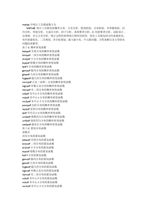
matlab中统计工具箱函数大全MATLAB统计工具箱包括概率分布、方差分析、假设检验、分布检验、非参数检验、回归分析、判别分析、主成分分析、因子分析、系统聚类分析、K均值聚类分析、试验设计、决策树、多元方差分析、统计过程控制和统计图形绘制等。
优化工具箱包括无约束最优化、有约束最优化、二次规划、多目标规划、最大最小化、半元限问题、方程求解以及大型优化问题的求解等。
表Ⅰ-1 概率密度函数betapdf贝塔分布的概率密度函数binopdf二项分布的概率密度函数chi2pdf卡方分布的概率密度函数exppdf指数分布的概率密度函数fpdf f分布的概率密度函数gampdf伽玛分布的概率密度函数geopdf几何分布的概率密度函数hygepdf超几何分布的概率密度函数normpdf正态(高斯)分布的概率密度函数lognpdf对数正态分布的概率密度函数nbinpdf负二项分布的概率密度函数ncfpdf非中心f分布的概率密度函数nctpdf非中心t分布的概率密度函数ncx2pdf非中心卡方分布的概率密度函数poisspdf泊松分布的概率密度函数raylpdf雷利分布的概率密度函数tpdf学生氏t分布的概率密度函数unidpdf离散均匀分布的概率密度函数unifpdf连续均匀分布的概率密度函数weibpdf威布尔分布的概率密度函数表Ⅰ-2 累加分布函数函数名对应分布的累加函数betacdf贝塔分布的累加函数binocdf二项分布的累加函数chi2cdf卡方分布的累加函数expcdf指数分布的累加函数fcdf f分布的累加函数gamcdf伽玛分布的累加函数geocdf几何分布的累加函数hygecdf超几何分布的累加函数logncdf对数正态分布的累加函数nbincdf负二项分布的累加函数ncfcdf非中心f分布的累加函数nctcdf非中心t分布的累加函数ncx2cdf非中心卡方分布的累加函数normcdf正态(高斯)分布的累加函数poisscdf泊松分布的累加函数raylcdf雷利分布的累加函数tcdf学生氏t分布的累加函数unidcdf离散均匀分布的累加函数unifcdf连续均匀分布的累加函数weibcdf威布尔分布的累加函数表Ⅰ-11 线性模型函数anova1单因子方差分析anova2双因子方差分析anovan多因子方差分析aoctool协方差分析交互工具dummyvar拟变量编码friedman Friedman检验glmfit一般线性模型拟合kruskalwallis Kruskalwallis检验leverage中心化杠杆值lscov已知协方差矩阵的最小二乘估计manova1单因素多元方差分析manovacluster多元聚类并用冰柱图表示multcompare多元比较多项式评价及误差区间估计polyfit最小二乘多项式拟合polyval多项式函数的预测值polyconf残差个案次序图regress多元线性回归regstats回归统计量诊断Ridge岭回归rstool多维响应面可视化robustfit稳健回归模型拟合stepwise逐步回归x2fx用于设计矩阵的因子设置矩阵表Ⅰ-12 非线性回归函数nlinfit非线性最小二乘数据拟合(牛顿法)nlintool非线性模型拟合的交互式图形工具nlparci参数的置信区间nlpredci预测值的置信区间nnls非负最小二乘表Ⅰ-13 试验设计函数cordexch D-优化设计(列交换算法)daugment递增D-优化设计dcovary固定协方差的D-优化设计ff2n二水平完全析因设计fracfact二水平部分析因设计fullfact混合水平的完全析因设计hadamard Hadamard矩阵(正交数组)rowexch D-优化设计(行交换算法)表Ⅰ-14 主成分分析函barttest Barttest检验pcacov源于协方差矩阵的主成分pcares源于主成分的方差princomp根据原始数据进行主成分分析表Ⅰ-15 多元统计函数classify聚类分析mahal马氏距离manova1单因素多元方差分析manovacluster多元聚类分析表Ⅰ-16 假设检验函数ranksum秩和检验signrank符号秩检验signtest符号检验ttest单样本t检验ttest2双样本t检验ztest z检验表Ⅰ-17 分布检验函数jbtest正态性的Jarque-Bera检验kstest单样本Kolmogorov-Smirnov检验kstest2双样本Kolmogorov-Smirnov检验lillietest正态性的Lilliefors检验Ⅰ-18 非参数函数friedman Friedman检验kruskalwallis Kruskalwallis检验ranksum秩和检验signrank符号秩检验signtest符号检验表Ⅰ-19 文件输入输出函数caseread读取个案名casewrite写个案名到文件tblread以表格形式读数据tblwrite以表格形式写数据到文件tdfread从表格间隔形式的文件中读取文本或数值数据表Ⅰ-20 演示函数aoctool协方差分析的交互式图形工具disttool探察概率分布函数的GUI工具glmdemo一般线性模型演示randtool随机数生成工具polytool多项式拟合工具rsmdemo响应拟合工具robustdemo稳健回归拟合工具统计工具箱是matlab提供给人们的一个强有力的统计分析工具.包含200多个m文件(函数),主要支持以下各方面的内容.〉〉概率分布:提供了20种概率分布,包含离散和连续分布,且每种分布,提供了5个有用的函数,即概率密度函数,累积分布函数,逆累积分布函数,随机产生器与方差计算函数.〉〉参数估计:依据特殊分布的原始数据,可以计算分布参数的估计值及其置信区间.〉〉描述性统计:提供描述数据样本特征的函数,包括位置和散布的度量,分位数估计值和数据处理缺失情况的函数等.〉〉线性模型:针对线性模型,工具箱提供的函数涉及单因素方差分析,双因素方差分析,多重线性回归,逐步回归,响应曲面和岭回归等.〉〉非线性模型:为非线性模型提供的函数涉及参数估计,多维非线性拟合的交互预测和可视化以及参数和预计值的置信区间计算等.〉〉假设检验: 此间提供最通用的假设检验函数:t检验和z检验〉〉其它的功能就不再介绍.统计工具箱函数主要分为两类:〉数值计算函数(M文件)〉交互式图形函数(Gui)matlab惯例:beta 线性模型中的参数,E(x) x的数学期望,f(x|a,b) 概率密度函数,F(x|a,b) 累积分布函数,I([a,b]) 指示(Indicator)函数p,q p事件发生的概率.[size=2][color=blue]第1节概率分布[/color][/size]统计工具箱提供的常见分布Uniform均匀,Weibull威布尔,Noncentral t,Rayleigh瑞利,Poisson泊松,Student's t,Normal 正态,Negative Binomial,Noncentral FLognormal对数,正态,Hyper G,F分布,Gamma,Geometric几何,Noncentral chi-square,Exponential指数,Binomial二项,Chi-squareBeta(分布),discrete,Continuous,Continuous,离散分布,统计量连续分布,数据连续分布,概率密度函数pdf,probbability density function〉〉功能:可选的通用概率密度函数〉〉格式:Y=pdf('Name',X,A1,A1,A3)'Name' 为特定的分布名称,第一个字母必须大写X 为分布函数自变量取值矩阵A1,A2,A3 分别为相应分布的参数值Y 存放结果,为概率密度值矩阵算例:>> y=pdf('Normal',-2:2,0,1)y =0.0540 0.2420 0.3989 0.2420 0.0540>> Y=pdf('Normal',-2:0.5:2,1,4)Y =0.0753 0.0820 0.0880 0.0930 0.0967 0.0990 0.0997 0.0990 0.0967>> p=pdf('Poisson',0:2:8,2)p =0.1353 0.2707 0.0902 0.0120 0.0009>> p=pdf('F',1:2:10,4,7)p =0.4281 0.0636 0.0153 0.0052 0.0021我们也可以利用这种计算功能和作图功能,绘制一下密度函数曲线,例如,绘制不同的正态分布的密度曲线>> x=[-6:0.05:6];>> y1=pdf('Normal',x,0,0.5);>> y2=pdf('Normal',x,0,1);>> y3=pdf('Normal',x,0,2);>> y4=pdf('Normal',x,0,4);>>plot(x,y1,'K-',x,y2,'K--',x,y3,'*',x,y4,'+')这个程序计算了mu=0,而sigma取不同值时的正态分布密度函数曲线的形态,可以看出,sigma 越大,曲线越平坦.累积分布函数及逆累积分布函数cdf icdf〉〉功能:计算可选分布函数的累积分布和逆累积分布函数〉〉格式:P=cdf('Name',X,A1,A2,A3)X=icdf('Name',P,A1,A2,A3)>> x=[-3:0.5:3];>> p=cdf('Normal',x,0,1)p =0.0013 0.0062 0.0228 0.0668 0.1587 0.3085 0.5000 0.6915 0.8413 0.9332 0.9772 0.9938 0.9987 >> x=icdf('Normal',p,0,1)x =-3.0000 -2.5000 -2.0000 -1.5000 -1.0000 -0.5000 0 0.5000 1.0000 1.5000 2.0000 2.5000 3.0000 随机数产生器random〉〉功能:产生可选分布的随机数〉〉格式:y=random('Name',A1,A2,A3,m,n)A1,A2,A3 分布的参数'Name' 分布的名称m,n 确定y的数量,如果参数是标量,则y是m*n矩阵例如产生服从参数为(9,10)的F-分布的4个随机数值>> y=random('F',9,10,2,2)y =3.4907 1.67620.5702 1.1534均值和方差以'stat'结尾的函数均值和方差的计算函数[m,v]=normstat(mu,sigma)正态分布[mn,v]=hygestat(M,K,N)超几何分布[m,v]=geostat(P)几何分布[m,v]=gamstat(A,B)Gamma分布[m,v]=fstat(v1,v2)F 分布[m,v]=expstat(mu)指数分布[m,v]=chi2stat(nu)Chi-squrare分布[m,v]=binostat(N,P)二项分布[m,v]=betastat(A,B)Beta 分布函数名称及调用格式分布类型名称[m,v]=weibstat(A,B)威尔分布[m,v]=unistat(A,B)连续均匀分布[m,v]=unidstat(N)离散均匀分布[m,v]=tstat(nu)t 分布[m,v]=raylstat(B)瑞利分布[m,v]=poisstat(lambda)泊松分布[m,v]=ncx2stat(nu,delta)非中心chi2分布[m,v]=nctstat(nu,delta)非中心t分布[m,v]=ncfstat(nu1,nu2,delta)非中心F分布[m,v]=nbinstat(R,P)负二项分布[m,v]=lognstat(mu,sigma)对数正态分布[size=2][color=blue]第2节参数估计[/color][/size]参数估计是总体的分布形式已经知道,且可以用有限个参数表示的估计问题.分为点估计(极大似燃估计Maximum likehood estimation, MLE)和区间估计.求取各种分布的最大似然估计估计量mle〉〉格式:phat=mle('dist',data)[phat,pci]=mle('dist',data)[phat,pci]=mle('dist',data,alpha)[phat,pci]=mle('dist',data,alpha,p1)〉〉'dist' 给定的特定分布的名称,'beta','binomial'等.Data为数据样本,矢量形式给出.Alpha用户给定的置信度值,以给出100(1-alpha)%的置信区间,缺省为0.05.最后一种是仅供二项分布参数估计,p1为实验次数.例1 计算beta 分布的两个参数的似然估计和区间估计(alpha=0.1,0.05,0.001),样本由随机数产生.>> random('beta',4,3,100,1);>> [p,pci]=mle('beta',r,0.1)p =4.6613 3.5719pci =3.6721 2.78115.6504 4.3626>> [p,pci]=mle('beta',r,0.05)p =4.6613 3.5719pci =3.4827 2.62965.8399 4.5141>> [p,pci]=mle('beta',r,0.001)p =4.6613 3.5719pci =2.6825 1.99006.6401 5.1538例2 计算二项分布的参数估计与区间估计,alpha=0.01.>> r=random('Binomial',10,0.2,10,1);>> [p,pci]=mle('binomial',r,0.01,10)p =0.2000 0.2000 0.1000 0.4000 0.2000 0.2000 0.4000 0 0.1000 0.2000pci =0.0109 0.0109 0.0005 0.0768 0.0109 0.0109 0.0768 NaN 0.0005 0.01090.6482 0.6482 0.5443 0.8091 0.6482 0.6482 0.8091 0.4113 0.5443 0.6482[size=2][color=blue] 第3节描述统计[/color][/size]描述性统计包括:位置度量,散布度量,缺失数据下的统计处理,相关系数,样本分位数,样本峰度, 样本偏度,自助法等〉〉位置度量:几何均值(geomean),调和均值(harmmean),算术平均值(mean),中位数(median),修正的样本均值(trimean).〉〉散布度量:方差(var),内四分位数间距(iqr),平均绝对偏差(mad),样本极差(range),标准差(std),任意阶中心矩(moment),协方差矩阵(cov).〉〉缺失数据情况下的处理:忽视缺失数据的最大值(nanmax),忽视缺失数据的平均值(nanmean),忽视缺失数据的中位数(nanmedian),忽视缺失数据的最小值(nanmin),忽视缺失数据的标准差(nanstd),忽视缺失数据的和(namsum).〉〉相关系数:corrcoef ,计算相关系数〉〉样本分位数:prctile,计算样本的经验分位数〉〉样本峰度:kurtosis,计算样本峰度〉〉样本偏度:skewness,计算样本偏度〉〉自助法:bootstrp,对样本从新采样进行自助统计中心趋势(位置)度量样本中心趋势度量的目的在于对数据样本在分布线上分布的中心位置予以定为.均值是对中心位置简单和通常的估计量.不幸的是,几乎所有的实际数据都存在野值(输入错误或其它小的技术问题造成的).样本均值对这样的值非常敏感.中位数和修正(剔除样本高值和低值)后的均值则受野值干扰很小.而几何均值和调和均值对野值也较敏感.下面逐个说明这些度量函数. 〉〉geomean功能:样本的几何均值格式:m=geomean(X)若X为向量,则返回X中元素的几何均值;若X位矩阵,给出的结果为一个行向量,即每列几何均值.例1 计算随机数产生的样本的几何均值>> X=random('F',10,10,100,1);>> m=geomean(X)m =1.1007>> X=random('F',10,10,100,5);>> m=geomean(X)m =0.9661 1.0266 0.9703 1.0268 1.0333〉〉harmmean功能:样本的调和均值格式:m=harmmean(X)例2 计算随机数的调和均值>> X=random('Normal',0,1,50,5);>> m=harmmean(X)m =-0.2963 -0.0389 -0.9343 5.2032 0.7122〉〉mean功能:样本数据的算术平均值格式:m=mean(x)例3 计算正态随机数的算术平均数>>X=random('Normal',0,1,300,5);>> xbar=mean(X)xbar =0.0422 -0.0011 -0.0282 0.0616 -0.0080〉〉median功能:样本数据的中值(中位数),是对中心位值的鲁棒估计.格式:m=median(X)例4 计算本的中值>> X=random('Normal',0,1,5,3)X =0.0000 0.8956 0.5689-0.3179 0.7310 -0.25561.0950 0.5779 -0.3775-1.8740 0.0403 -0.29590.4282 0.6771 -1.4751>> m=median(X)m =0.0000 0.6771 -0.2959〉〉trimmean功能:剔除极端数据的样本均值.格式:m=trimmean(X,percent)说明:计算剔除观测值中最高percent%和最低percent%的数据后的均值例5 计算修改后的样本均值>> X=random('F',9,10,100,4);>> m=trimmean(X,10)m =1.1470 1.1320 1.1614 1.0469散布度量散布度量是描述样本中数据离其中心的程度,也称离差.常用的有极差,标准差,平均绝对差,四分位数间距〉〉iqr功能:计算样本的内四分位数的间距,是样本的鲁棒估计格式:y=iqr(X)说明:计算样本的75%和25%的分位数之差,不受野值影响.例6 计算样本的四分位间距>> X=random('Normal',0,1,100,4);>> m=iqr(X)m =1.3225 1.2730 1.3018 1.2322〉〉mad功能:样本数据的平均绝对偏差格式:y=mad(X)说明:正态分布的标准差sigma可以用mad乘以1.3估计例7 计算样本数据的绝对偏差>> X=random('F',10,10,100,4);>> y=mad(X)y =0.5717 0.5366 0.6642 0.7936>> y1=var(X)y1 =0.6788 0.6875 0.7599 1.3240>> y2=y*1.3y2 =0.8824 0.8938 0.9879 1.7212〉〉range功能:计算样本极差格式:y=range(X)说明:极差对野值敏感例8 计算样本值的极差>> X=random('F',10,10,100,4);>> y=range(X)y =10.8487 3.5941 4.2697 4.0814〉〉var功能:计算样本方差格式:y=var(X) y=var(X,1) y=var(X,w)Var(X)经过n-1进行了标准化,Var(X,1)经过n进行了标准变化例9 计算各类方差>> X=random('Normal',0,1,100,4);>> y=var(X)y =0.9645 0.8209 0.9595 0.9295>> y1=var(X,1)y1 =0.9548 0.8126 0.9499 0.9202>> w=[1:1:100];>> y2=var(X,w)y2 =0.9095 0.7529 0.9660 0.9142〉〉std功能:样本的标准差格式:y=std(X)说明:经过n-1标准化后的标准差例10计算随机样本的标准差>> X=random('Normal',0,1,100,4);>> y=std(X)y =0.8685 0.9447 0.9569 0.9977〉〉cov功能:协方差矩阵格式:C=cov(X) C=cov(x,y) C=cov([x y])说明:若X为向量,cov(X)返回一个方差标量;若X为矩阵,则返回协方差矩阵;cov(x,y)与cov([x y])相同,x与y的长度相同.例11 计算协方差>> x=random('Normal',2,4,100,1);>> y=random('Normal',0,1,100,1);>> C=cov(x,y)C =12.0688 -0.0583-0.0583 0.8924处理缺失数据的函数在对大量数据样本时,常常遇到一些无法确定的或者无法找到确切的值.在这种情况下,用符号"NaN"(not a number )标注这样的数据.这种情况下,一般的函数得不到任何信息.例如m中包含nan数据>> m=magic(3);>> m([1 5 9])=[NaN NaN NaN];>> sum(m)ans =NaN NaN NaN但是通过缺失数据的处理,得到有用的信息.>> nansum(m)ans =7 10 13〉〉nanmax功能:忽视NaN,求其它数据的最大值格式:m=nanmax(X)[m,ndx]=nanmax(X)m=nanmax(a,b)说明:nanmax(X)返回X中数据除nan外的其它的数据的最大值,[m,ndx]=nanmax(X)还返回X 最大值的序号给ndx.m=nanmax(a,b)返回a或者b的最大值,a,b长度同>> m=magic(3);>> m([1 5 9])=[NaN NaN NaN];>> [m,ndx]=nanmax(m)m =4 9 7ndx =3 3 2处理缺失数据的常用函数Y=nansum(X)求包含确实数据的和nansumY=nanstd(X)求包含确实数据的标准差NanstdY=nanmedian(X)求包含确实数据中位数NanmedianY=nanmean(X)求包含确实数据的平均值Nanmean同上求包含确实数据的最小值Nanmin(略)求包含确实数据的最大值Nanmax调用格式功能函数名称中心矩moment功能:任意阶的中心矩格式:m=moment(X,order)说明:order为阶,函数本身除以X的长度例12 计算样本函数的中心矩>> X=random('Poisson',2,100,4);>> m=moment(X,1)m =0 0 0 0>> m=moment(X,2)m =1.76042.0300 1.6336 2.3411>> m=moment(X,3)m =1.37792.5500 2.3526 2.2964百分位数及其图形描述白分位数图形可以直观观测到样本的大概中心位置和离散程度,可以对中心趋势度量和散布度量作补充说明〉〉prctile功能:计算样本的百分位数格式:y=prctile(X,p)说明:计算X中数据大于P%的值,P的取值区间为[0,100],如果X为向量,返回X中P百分位数;X 为矩阵,给出一个向量;如果P为向量,则y的第i个行对应于X的p(i) 百分位数.例如>> x=(1:5)'*(1:5)x =1 2 3 4 52 4 6 8 103 6 9 12 154 8 12 16 205 10 15 20 25>> y=prctile(x,[25,50,75])y =1.7500 3.5000 5.2500 7.0000 8.75003.0000 6.0000 9.0000 12.0000 15.00004.2500 8.5000 12.7500 17.0000 21.2500做出相应的百分位数的图形>> boxplot(x)5列分位数构造5个盒图,见下页.相关系数corrcoef功能:相关系数格式:R=corrcoef(X)例13 合金的强度y与含碳量x的样本如下,试计算r(x,y).>> X=[41 42.5 45 45.5 45 47.5 49 51 50 55 57.5 59.5;0.1,0.11 0.12 0.13 0.14 0.15 0.16 0.17 0.18 0.20 0.22 0.24]';>> R=corrcoef(X)R =1.0000 0.98970.9897 1.0000样本峰度kurtosis功能:样本峰度格式:k=kurtosis(X)说明:峰度为单峰分布区线" 峰的平坦程度"的度量,其定义为Matlab 工具箱中峰度不采用一般定义(k-3,标准正态分布的峰度为0).而是定义标准正态分布峰度为3,曲线比正态分布平坦,峰度大于3,反之,小于3.例14 计算随机样本的峰度>> X=random('F',10,20,100,4);>> k=kurtosis(X)k =6.5661 5.58516.03497.0129样本偏度skewness功能:样本偏度格式:y=skewness(X)说明:偏度是度量样本围绕其均值的对称情况.如果偏度为负,则数据分布偏向左边,反之,偏向右边.其定义为>> X=random('F',9,10,100,4);>> y=skewness(X)y =1.0934 1.55132.0522 2.9240自助法bootstrap引例:一组来自15个法律学校的学生的lsat分数和gpa进行比较的样本.> load lawdata>> x=[lsat gpa]x =576.0000 3.3900635.0000 3.3000558.0000 2.8100578.0000 3.0300666.0000 3.4400580.0000 3.0700555.0000 3.0000661.0000 3.4300651.0000 3.3600605.0000 3.1300653.0000 3.1200575.0000 2.7400545.0000 2.7600572.0000 2.8800594.0000 2.9600绘图,并进行曲线拟合>> plot(lsat,gpa,'+')>> lsline通过上图的拟合可以看出,lsat随着gpa增长而提高,但是我们确信此结论的程度是多少曲线只给出了直观表现,没有量的表示.计算相关系数>> y=corrcoef(lsat,gpa)y =1.0000 0.77640.7764 1.0000相关系数是0.7764,但是由于样本容量n=15比较小,我们仍然不能确定在统计上相关的显著性多大.应此,必须采用bootstrp函数对lsat和gpa样本来从新采样,并考察相关系数的变化. >> y1000=bootstrp(1000,'corrcoef',lsat,gpa);>> hist(y1000(:,2),30)绘制lsat,gpa和相关系数得直方图如下结果显示,相关系数绝大多数在区间[0.4,1] 内,表明lsat分数和gpa具有确定的相关性,这样的分析,不需要对象关系数的概率分布做出很强的假设.[size=2] [color=blue]第4节假设检验[/color][/size]基本概念H0:零假设,即初始判断.H1:备择假设, 也称对立假设.Alpha :显著水平,在小样本的前提下,不能肯定自己的结论,所以事先约定,如果观测到的符合零假设的样本值的概率小于alpha,则拒绝零假设.典型的显著水平取alpha=0.05.如果想减少犯错误的可能,可取更小的值.P-值:在零假设为真的条件下,观测给定样本结果的概率值.如果Pmu tail=-1——x>x =[119 117 115 116 112 121 115 122 116 118 109 112 119 112 117 113 114 109 109 118];>> h=ztest(x,115,4)h =表明,接受H0,认为该种汽油的平均价格为115美分.>> [h,sig,ci]=ztest(x,115,4,0.01,0)h = 0sig =0.8668ci =112.8461 117.4539>> [h,sig,ci]=ztest(x,115,4,0.01,1)h =0sig =0.4334ci =113.0693 Inf>> [h,sig,ci]=ztest(x,115,4,0.01,-1)h=0sig =0.5666ci =-Inf 117.2307Ttest功能:单一样本均值的t检验格式:h=ttest(x,m)h=ttest(x,m,alpha)[h,sig,ci]=ttest(x,m,alpha,tail)说明:用于正态总体标准差未知时对均值的t检验.Tail功能与ztest作用一致.>> x=random('Normal',0,1,100,1);>> [h,sig,ci]=ttest(x,0,0.01,-1)h =sig =0.0648ci =-Inf 0.0808>> [h,sig,ci]=ttest(x,0,0.001,1)h =sig =0.9352ci =-0.4542 InfSigntest功能:成对样本的符号检验格式:p=signtest(x,y,alpha)[p,h]=signtest(x,y,alpha)说明:p给出两个配对样本x和y的中位数(对于正态分布,中位数,就是平均值.相等的显著性概率.X与y的长度相等.Y也可以为标量,计算x的中位数与常数y之间差异的概率.[p,h]返回结果h.如果这样两个样本的中位数之间差几乎为0,则h=0,否则有显著差异,则h=1.>> x=[0 1 0 1 1 1 1 0 1 0];>> y=[1 1 0 0 0 0 1 1 0 0];>> [p,h]=signtest(x,y,0.05)p =0.6875h =Signrank功能:威尔科克符号秩检验格式:p=signrank(x,y,alpha)[p,h]=signrank(x,y,alpha)说明:p给出两个配对样本x和y的中位数(对于正态分布,中位数和均值等)相等的假设的显著性的概率.X与y的长度相同.[p,h]返回假设检验的结果,如果两个样本的中位数之差极护卫零,则h=0;否则,有显著差异,则h=1.>> x=random('Normal',0,1,200,1);>> y=random('Normal',0.1,2,200,1);>> [p,h]=signrank(x,y,0.05)p =0.9757h =Ranksum功能:两个总体一致性的威尔科克秩和的检验格式:p=ranksum(x,y,alpha)[p,h]=ranksum(x,y,alpha)说明:p返回两个总体样本x和y一致的显著性概率.X和y的长度可以不同.但长度长的排在前面.[p,h]返回检验结果,如果总体x和y并非明显不一致,返回h=0,否则,h=1.>> x=random('Normal',0,2,20,1);>> y=random('Normal',0.1,4,10,1);>> [p,h]=ranksum(x,y,0.05)p =0.7918h =[size=2] [color=blue]第5节统计绘图[/color][/size]统计绘图就是用图形表达函数,以便直观地,充分的表现样本及其统计量的内在本质性. Box图功能:数据样本的box图格式:boxplot(X) boxplot(X,notch) boxplot(X,notch,'sym')boxplot(X,notch,'sym,vert) boxplot(X,notch,'sym',vert,whis)说明1:"盒子"的上底和下底间为四分位间距,"盒子"的上下两条线分别表示样本的25%和75%分位数."盒子"中间线为样本中位数.如果盒子中间线不在盒子中间,表示样本存在一定的篇度.虚线贯穿"盒子"上下,表示样本的其余部分(除非有野值).样本最大值为虚线顶端,样本最小值为虚线底端.用"+"表示野值."切口"是样本的置信区间,却省时,没有切口说明2:notch=0,盒子没有切口,notch=1,盒子有切口;'sym'为野值标记符号,缺省时,"+"表示.Vert=0时候,box图水平放置,vert=1时,box图垂直放置.Whis定义虚线长度为内四分位间距(IQR)的函数(缺省时为1.5*IQR),若whis=0,box图用'sym'规定的记号显示盒子外所有数据. >> x1=random('Normal',2,1,100,1);>> x2=random('Normal',1,2,100,1);>> x=[x1 x2];>> boxplot(x,1,'*',1,0)绘图结果见下页Errorbar 误差条图功能:误差条图格式:errorbar(X,Y,L,U,symbol)errorbar(X,Y,L)errorbar(Y,L)说明:误差条是距离点(X,Y)上面的长度为U(i) ,下面的长度为L(i) 的直线.X,Y,L,U的长度必须相同.Symbol为一字符串,可以规定线条类型,颜色等.>> U=ones(20,1);>> L=ones(20,1);>> errorbar(r1,r2,L,U,'+')>> r1=random('Poisson',2,10,1);>>r2=random('Poisson',10,10,1);>> U=ones(10,1);>> L=U;>> errorbar(r1,r2,L,U,'+')Lsline 绘制最小二乘拟合线功能:绘制数据的最小二乘拟合曲线格式:lslineh=lsline说明:lsline为当前坐标系中的每一个线性数据给出其最小二乘拟合线.>> y=[2 3.4 5.6 8 11 12.3 13.8 16 18.8 19.9]';>> plot(y,'+')>> lslineRefcurve 参考多项式功能:在当前图形中给出多项式拟合曲线格式:h=refcurve(p)说明:在当前图形中给出多项式p(系数向量)的曲线,n阶多项式为y=p1*x^n+p2*x^(n-1)+…+pn*x+p0则p=[p1 p2 … pn p0]>> h=[85 162 230 289 339 381 413 437 452 458 456 440 400 356];>> plot(h,'+')>> refcurve([-4.9,100,0])。
2、MATLAB统计工具箱中的回归分析命令
1.多元线性回归 . 2.多项式回归 . 3.非线性回归 4.逐步回归 .
返回
多元线性回归
y = β 0 + β 1 x1 + ... + β p x p
1.确定回归系数的点估计值: .确定回归系数的点估计值:
b=regress( Y,
ˆ β0 ˆ β1 b= M β ˆ p
由下列 4 个模型中选择 1 个(用字符串输入,缺省时为线性模型): linear(线性): y = β 0 + β 1 x1 + L + β m x m purequadratic(纯二次): interaction(交叉): y =
y = β 0 + β 1 x1 + L + β m x m + ∑ β jj x 2 j
x=[143 145 146 147 149 150 153 154 155 156 157 158 159 160 162 164]'; X=[ones(16,1) x]; Y=[88 85 88 91 92 93 93 95 96 98 97 96 98 99 100 102]';
2.回归分析及检验: .回归分析及检验: [b,bint,r,rint,stats]=regress(Y,X) b,bint,stats To MATLAB(liti11)
r2=0.9282, F=180.9531, p=0.0000 p<0.05, 可知回归模型 y=-16.073+0.7194x 成立.
3.残差分析,作残差图: .残差分析,作残差图: rcoplot(r,rint) 从残差图可以看出,除第二个数据外,其余数据的残 差离零点均较近,且残差的置信区间均包含零点,这说明 回归模型 y=-16.073+0.7194x能较好的符合原始数据,而第 二个数据可视为异常点.
Matlab统计工具箱简介
6
二 概率分布
随机变量的统计行为取决于其概率分布,而分布函数常用连续和 离散型分布。统计工具箱提供20种分布。每种分布有五类函数。
1: 概率密度(pdf) ; 2: 累积分布函数(cdf); 3:逆累积分布函数 (icdf);4: 随机数产生器 5: 均值和方差函数;
28
4.6中心矩
中心矩是关于数学期望的矩。对于任意的r 0,称
E(x)r
为随机变量X的r阶中心矩。一阶中心矩为0,二阶中心
矩为方差:
2 DX
函数moment计算任意阶中心矩。 格式:m=moment(X,order) 说明:order确定阶。
29
4.7相关系数
相关系数是两个随机变量间线性相依程度的 度量。
(如binomial二项分布,
n b(k;n,p)kpk(1p)nk
即n次贝努里试验中出现k次成功的概率.poisson
分布,
p(;k)
k
e
k!
4
1.1.2 概率分布—连续型
连续型分布
如正态分布F(x)=
( y)2
1
x
2
e
2
dy
beta分布,uniform平均分布等.
每种分布提供5类函数:
1 概率密度
25
4.3散布度量
散布度量可以理解为样本中的数据偏离其数值中心的 程度,也称离差。
极差,定义为样本最大观测值与最小观测值之差。 标准差和方差为常用的散布度量,对正态分布的样本
描述是最优的。但抗野值干扰能力较小。 平均绝对值偏差对野值也敏感。 四分位数间距为随机变量的上四分位数 和下四分位之
利用MATLAB进行统计分析
利用MATLAB进行统计分析使用 MATLAB 进行统计分析引言统计分析是一种常用的数据分析方法,可以帮助我们理解数据背后的趋势和规律。
MATLAB 提供了一套强大的统计工具箱,可以帮助用户进行数据的统计计算、可视化和建模分析。
本文将介绍如何利用 MATLAB 进行统计分析,并以实例展示其应用。
一、数据导入和预处理在开始统计分析之前,首先需要导入数据并进行预处理。
MATLAB 提供了多种导入数据的方式,可以根据实际情况选择合适的方法。
例如,可以使用`readtable` 函数导入Excel 表格数据,或使用`csvread` 函数导入CSV 格式的数据。
导入数据后,我们需要对数据进行预处理,以确保数据的质量和准确性。
预处理包括数据清洗、缺失值处理、异常值处理等步骤。
MATLAB 提供了丰富的函数和工具,可以帮助用户进行数据预处理。
例如,可以使用 `fillmissing` 函数填充缺失值,使用 `isoutlier` 函数识别并处理异常值。
二、描述统计分析描述统计分析是对数据的基本特征进行概括和总结的方法,可以帮助我们了解数据的分布、中心趋势和变异程度。
MATLAB 提供了多种描述统计分析的函数,可以方便地计算数据的均值、标准差、方差、分位数等指标。
例如,可以使用 `mean` 函数计算数据的均值,使用 `std` 函数计算数据的标准差,使用 `median` 函数计算数据的中位数。
此外,MATLAB 还提供了 `histogram`函数和 `boxplot` 函数,可以绘制数据的直方图和箱线图,从而更直观地展现数据的分布特征。
三、假设检验假设检验是统计分析中常用的推断方法,用于检验关于总体参数的假设。
MATLAB 提供了多种假设检验的函数,可以帮助用户进行单样本检验、双样本检验、方差分析等分析。
例如,可以使用 `ttest` 函数进行单样本 t 检验,用于检验一个总体均值是否等于某个给定值。
可以使用 `anova1` 函数进行单因素方差分析,用于比较不同组之间的均值差异是否显著。
Matlab数理统计工具箱常用函数命令大全
Matlab数理统计工具箱应用简介1.概述Matlab的数理统计工具箱是Matlab工具箱中较为简单的一个,其牵扯的数学知识是大家都很熟悉的数理统计,因此在本文中,我们将不再对数理统计的知识进行重复,仅仅列出数理统计工具箱的一些函数,这些函数的意义都很明确,使用也很简单,为了进一步简明,本文也仅仅给出了函数的名称,没有列出函数的参数以及使用方法,大家只需简单的在Matlab工作空间中输入“help 函数名”,便可以得到这些函数详细的使用方法。
2.参数估计betafit 区间3.累积分布函数betacdf β累积分布函数binocdf 二项累积分布函数cdf 计算选定的累积分布函数chi2cdf 累积分布函数2χexpcdf 指数累积分布函数fcdf F累积分布函数gamcdf γ累积分布函数geocdf 几何累积分布函数hygecdf 超几何累积分布函数logncdf 对数正态累积分布函数nbincdf 负二项累积分布函数ncfcdf 偏F累积分布函数nctcdf 偏t累积分布函数ncx2cdf 偏累积分布函数2χnormcdf 正态累积分布函数poisscdf 泊松累积分布函数raylcdf Reyleigh累积分布函数tcdf t 累积分布函数unidcdf 离散均匀分布累积分布函数unifcdf 连续均匀分布累积分布函数weibcdf Weibull累积分布函数4.概率密度函数betapdf β概率密度函数binopdf 二项概率密度函数chi2pdf 概率密度函数2χexppdf 指数概率密度函数fpdf F概率密度函数gampdf γ概率密度函数geopdf 几何概率密度函数hygepdf 超几何概率密度函数lognpdf 对数正态概率密度函数nbinpdf 负二项概率密度函数ncfpdf 偏F概率密度函数nctpdf 偏t概率密度函数ncx2pdf 偏概率密度函数2χnormpdf 正态分布概率密度函数pdf 指定分布的概率密度函数poisspdf 泊松分布的概率密度函数raylpdf Rayleigh概率密度函数tpdf t概率密度函数unidpdf 离散均匀分布概率密度函数unifpdf 连续均匀分布概率密度函数weibpdf Weibull概率密度函数5.逆累积分布函数Betainv 逆β累积分布函数binoinv 逆二项累积分布函数chi2inv 逆累积分布函数2χexpinv 逆指数累积分布函数finv 逆F累积分布函数gaminv 逆γ累积分布函数geoinv 逆几何累积分布函数hygeinv 逆超几何累积分布函数logninv 逆对数正态累积分布函数nbininv 逆负二项累积分布函数ncfinv 逆偏F累积分布函数nctinv 逆偏t累积分布函数ncx2inv 逆偏累积分布函数2χnorminv 逆正态累积分布函数possinv 逆正态累积分布函数raylinv 逆Rayleigh累积分布函数tinv 逆t累积分布函数unidinv 逆离散均匀累积分布函数unifinv 逆连续均匀累积分布函数weibinv 逆Weibull累积分布函数6.分布矩函数betastat 计算β分布的均值和方差binostat 二项分布的均值和方差chi2stat 计算分布的均值和方差2χexpstat 计算指数分布的均值和方差fstat 计算F分布的均值和方差gemstat 计算γ分布的均值和方差geostat 计算几何分布的均值和方差hygestat 计算超几何分布的均值和方差lognstat 计算对数正态分布的均值和方差nbinstat 计算负二项分布的均值和方差ncfstat 计算偏F分布的均值和方差nctstat 计算偏t分布的均值和方差ncx2stat 计算偏分布的均值和方差2χnormstat 计算正态分布的均值和方差poissstat 计算泊松分布的均值和方差raylstat 计算Rayleigh分布的均值和方差tstat 计算t分布的均值和方差unidstat 计算离散均匀分布的均值和方差unifstat 计算连续均匀分布的均值和方差weibstat 计算Weibull分布的均值和方差7.统计特征函数corrcoef 计算互相关系数cov 计算协方差矩阵geomean 计算样本的几何平均值harmmean 计算样本数据的调和平均值iqr 计算样本的四分位差kurtosis 计算样本的峭度mad 计算样本数据平均绝对偏差mean 计算样本的均值median 计算样本的中位数moment 计算任意阶的中心矩prctile 计算样本的百份位数range 样本的范围skewness 计算样本的歪度std 计算样本的标准差trimmean 计算包含极限值的样本数据的均值var 计算样本的方差8.统计绘图函数boxplot 在矩形框内画样本数据errorbar 在曲线上画误差条fsurfht 画函数的交互轮廓线gline 在图中交互式画线gname 用指定的标志画点lsline 画最小二乘拟合线normplot 画正态检验的正态概率图pareto 画统计过程控制的Pareto图qqplot 画两样本的分位数-分位数图refcurve 在当前图中加一多项式曲线refline 在当前坐标中画参考线surfht 画交互轮廓线weibplot 画Weibull概率图9.统计处理控制capable 处理能力索引capaplot 画处理能力图ewmaplot 画指数加权移动平均图histfit 叠加正态密度直方图normspec 在规定的极限内画正态密度图schart 画标准偏差图xbarplot 画水平条图10.假设检验Ranksum 计算母体产生的两独立样本的显著性概率和假设检验的结果signrank 计算两匹配样本中位数相等的显著性概率和假设检验的结果signtest 计算两匹配样本的显著性概率和假设检验的结果ttest 对单个样本均值进行t检验ttest2 对两样本均值差进行t检验ztest 对已知方差的单个样本均值进行z检验11.试验设计cordexch 配位交叉算法D-优化试验设计daugment D-优化增强试验设计dcovary 使用指定协变数的D-优化试验设计ff2n 两水平全因素试验设计fullfact 全因素试验设计hadamard Hadamard正交试验rowexch 行交换算法D-优化试验设计。
MATLAB常用工具箱与函数库介绍
MATLAB常用工具箱与函数库介绍1. 统计与机器学习工具箱(Statistics and Machine Learning Toolbox):该工具箱提供了各种统计分析和机器学习算法的函数,包括描述统计、概率分布、假设检验、回归分析、分类与聚类等。
可以用于进行数据探索和建模分析。
2. 信号处理工具箱(Signal Processing Toolbox):该工具箱提供了一系列信号处理的函数和算法,包括滤波、谱分析、信号生成与重构、时频分析等。
可以用于音频处理、图像处理、通信系统设计等领域。
3. 控制系统工具箱(Control System Toolbox):该工具箱提供了控制系统设计与分析的函数和算法,包括系统建模、根轨迹设计、频域分析、状态空间分析等。
可以用于控制系统的设计和仿真。
4. 优化工具箱(Optimization Toolbox):该工具箱提供了各种数学优化算法,包括线性规划、非线性规划、整数规划、最优化等。
可以用于寻找最优解或最优化问题。
5. 图像处理工具箱(Image Processing Toolbox):该工具箱提供了图像处理和分析的函数和算法,包括图像滤波、边缘检测、图像分割、图像拼接等。
可以用于计算机视觉、医学影像处理等领域。
6. 神经网络工具箱(Neural Network Toolbox):该工具箱提供了神经网络的建模和训练工具,包括感知机、多层前馈神经网络、循环神经网络等。
可以用于模式识别、数据挖掘等领域。
7. 控制系统设计工具箱(Robust Control Toolbox):该工具箱提供了鲁棒控制系统设计与分析的函数和算法,可以处理不确定性和干扰的控制系统设计问题。
8. 信号系统工具箱(Signal Systems Toolbox):该工具箱提供了分析、设计和模拟线性时不变系统的函数和算法。
可以用于信号处理、通信系统设计等领域。
9. 符号计算工具箱(Symbolic Math Toolbox):该工具箱提供了符号计算的功能,可以进行符号表达式的运算、求解方程、求解微分方程等。
- 1、下载文档前请自行甄别文档内容的完整性,平台不提供额外的编辑、内容补充、找答案等附加服务。
- 2、"仅部分预览"的文档,不可在线预览部分如存在完整性等问题,可反馈申请退款(可完整预览的文档不适用该条件!)。
- 3、如文档侵犯您的权益,请联系客服反馈,我们会尽快为您处理(人工客服工作时间:9:00-18:30)。
% Statistics Toolbox% betafit - Beta parameter estimation.% binofit - Binomial parameter estimation.% dfittool - Distribution fitting tool.% evfit - Extreme value parameter estimation.% expfit - Exponential parameter estimation.% gamfit - Gamma parameter estimation.% lognfit - Lognormal parameter estimation.% mle - Maximum likelihood estimation (MLE).% mlecov - Asymptotic covariance matrix of MLE.% nbinfit - Negative binomial parameter estimation.% normfit - Normal parameter estimation.% poissfit - Poisson parameter estimation.% raylfit - Rayleigh parameter estimation.% unifit - Uniform parameter estimation.% wblfit - Weibull parameter estimation.%% Probability density functions (pdf).% betapdf - Beta density.% binopdf - Binomial density.% chi2pdf - Chi square density.% evpdf - Extreme value density.% exppdf - Exponential density.% fpdf - F density.% gampdf - Gamma density.% geopdf - Geometric density.% hygepdf - Hypergeometric density.% lognpdf - Lognormal density.% mvnpdf - Multivariate normal density.% nbinpdf - Negative binomial density.% ncfpdf - Noncentral F density.% nctpdf - Noncentral t density.% ncx2pdf - Noncentral Chi-square density.% normpdf - Normal (Gaussian) density.% pdf - Density function for a specified distribution. % poisspdf - Poisson density.% raylpdf - Rayleigh density.% tpdf - T density.% unidpdf - Discrete uniform density.% unifpdf - Uniform density.% wblpdf - Weibull density.%% Cumulative Distribution functions (cdf).% betacdf - Beta cdf.% binocdf - Binomial cdf.% cdf - Specified cumulative distribution function.% chi2cdf - Chi square cdf.% ecdf - Empirical cdf (Kaplan-Meier estimate).% evcdf - Extreme value cumulative distribution function.% expcdf - Exponential cdf.% fcdf - F cdf.% gamcdf - Gamma cdf.% geocdf - Geometric cdf.% hygecdf - Hypergeometric cdf.% logncdf - Lognormal cdf.% nbincdf - Negative binomial cdf.% ncfcdf - Noncentral F cdf.% nctcdf - Noncentral t cdf.% ncx2cdf - Noncentral Chi-square cdf.% normcdf - Normal (Gaussian) cdf.% poisscdf - Poisson cdf.% raylcdf - Rayleigh cdf.% tcdf - T cdf.% unidcdf - Discrete uniform cdf.% unifcdf - Uniform cdf.% wblcdf - Weibull cdf.%% Critical Values of Distribution functions.% betainv - Beta inverse cumulative distribution function.% binoinv - Binomial inverse cumulative distribution function.% chi2inv - Chi square inverse cumulative distribution function.% evinv - Extreme value inverse cumulative distribution function.% expinv - Exponential inverse cumulative distribution function.% finv - F inverse cumulative distribution function.% gaminv - Gamma inverse cumulative distribution function.% geoinv - Geometric inverse cumulative distribution function.% hygeinv - Hypergeometric inverse cumulative distribution function.% icdf - Specified inverse cdf.% logninv - Lognormal inverse cumulative distribution function.% nbininv - Negative binomial inverse distribution function.% ncfinv - Noncentral F inverse cumulative distribution function.% nctinv - Noncentral t inverse cumulative distribution function.% ncx2inv - Noncentral Chi-square inverse distribution function.% norminv - Normal (Gaussian) inverse cumulative distribution function. % poissinv - Poisson inverse cumulative distribution function.% raylinv - Rayleigh inverse cumulative distribution function.% tinv - T inverse cumulative distribution function.% unidinv - Discrete uniform inverse cumulative distribution function.% unifinv - Uniform inverse cumulative distribution function. % wblinv - Weibull inverse cumulative distribution function. %% Random Number Generators.% betarnd - Beta random numbers.% binornd - Binomial random numbers.% chi2rnd - Chi square random numbers.% evrnd - Extreme value random numbers.% exprnd - Exponential random numbers.% frnd - F random numbers.% gamrnd - Gamma random numbers.% geornd - Geometric random numbers.% hygernd - Hypergeometric random numbers.% iwishrnd - Inverse Wishart random matrix.% lognrnd - Lognormal random numbers.% mvnrnd - Multivariate normal random numbers.% mvtrnd - Multivariate t random numbers.% nbinrnd - Negative binomial random numbers.% ncfrnd - Noncentral F random numbers.% nctrnd - Noncentral t random numbers.% ncx2rnd - Noncentral Chi-square random numbers.% normrnd - Normal (Gaussian) random numbers.% poissrnd - Poisson random numbers.% randg - Gamma random numbers (unit scale).% random - Random numbers from specified distribution.% randsample - Random sample from finite population.% raylrnd - Rayleigh random numbers.% trnd - T random numbers.% unidrnd - Discrete uniform random numbers.% unifrnd - Uniform random numbers.% wblrnd - Weibull random numbers.% wishrnd - Wishart random matrix.%% Statistics.% betastat - Beta mean and variance.% binostat - Binomial mean and variance.% chi2stat - Chi square mean and variance.% evstat - Extreme value mean and variance.% expstat - Exponential mean and variance.% fstat - F mean and variance.% gamstat - Gamma mean and variance.% geostat - Geometric mean and variance.% hygestat - Hypergeometric mean and variance.% lognstat - Lognormal mean and variance.% nbinstat - Negative binomial mean and variance.% ncfstat - Noncentral F mean and variance.% nctstat - Noncentral t mean and variance.% ncx2stat - Noncentral Chi-square mean and variance.% normstat - Normal (Gaussian) mean and variance.% poisstat - Poisson mean and variance.% raylstat - Rayleigh mean and variance.% tstat - T mean and variance.% unidstat - Discrete uniform mean and variance.% unifstat - Uniform mean and variance.% wblstat - Weibull mean and variance.%% Likelihood functions.% betalike - Negative beta log-likelihood.% evlike - Negative extreme value log-likelihood.% explike - Negative exponential log-likelihood.% gamlike - Negative gamma log-likelihood.% lognlike - Negative lognormal log-likelihood.% nbinlike - Negative likelihood for negative binomial distribution. % normlike - Negative normal likelihood.% wbllike - Negative Weibull log-likelihood.%% Descriptive Statistics.% bootstrp - Bootstrap statistics for any function.% corr - Linear or rank correlation coefficient.% corrcoef - Linear correlation coefficient with confidence intervals. % cov - Covariance.% crosstab - Cross tabulation.% geomean - Geometric mean.% grpstats - Summary statistics by group.% harmmean - Harmonic mean.% iqr - Interquartile range.% kurtosis - Kurtosis.% mad - Median Absolute Deviation.% mean - Sample average (in MATLAB toolbox).% median - 50th percentile of a sample.% moment - Moments of a sample.% nanmax - Maximum ignoring NaNs.% nanmean - Mean ignoring NaNs.% nanmedian - Median ignoring NaNs.% nanmin - Minimum ignoring NaNs.% nanstd - Standard deviation ignoring NaNs.% nansum - Sum ignoring NaNs.% nanvar - Variance ignoring NaNs.% prctile - Percentiles.% quantile - Quantiles.% range - Range.% skewness - Skewness.% std - Standard deviation (in MATLAB toolbox).% tabulate - Frequency table.% trimmean - Trimmed mean.% var - Variance (in MATLAB toolbox).%% Linear Models.% addedvarplot - Created added-variable plot for stepwise regression.% anova1 - One-way analysis of variance.% anova2 - Two-way analysis of variance.% anovan - n-way analysis of variance.% aoctool - Interactive tool for analysis of covariance.% dummyvar - Dummy-variable coding.% friedman - Friedman's test (nonparametric two-way anova).% glmfit - Generalized linear model fitting.% glmval - Evaluate fitted values for generalized linear model.% kruskalwallis - Kruskal-Wallis test (nonparametric one-way anova).% leverage - Regression diagnostic.% lscov - Least-squares estimates with known covariance matrix.% lsqnonneg - Non-negative least-squares.% manova1 - One-way multivariate analysis of variance.% manovacluster - Draw clusters of group means for manova1.% multcompare - Multiple comparisons of means and other estimates.% polyconf - Polynomial evaluation and confidence interval estimation.% polyfit - Least-squares polynomial fitting.% polyval - Predicted values for polynomial functions.% rcoplot - Residuals case order plot.% regress - Multivariate linear regression.% regstats - Regression diagnostics.% ridge - Ridge regression.% robustfit - Robust regression model fitting.% rstool - Multidimensional response surface visualization (RSM).% stepwise - Interactive tool for stepwise regression.% stepwisefit - Non-interactive stepwise regression.% x2fx - Factor settings matrix (x) to design matrix (fx).%% Nonlinear Models.% nlinfit - Nonlinear least-squares data fitting.% nlintool - Interactive graphical tool for prediction in nonlinear models. % nlpredci - Confidence intervals for prediction.% nlparci - Confidence intervals for parameters.%% Design of Experiments (DOE).% bbdesign - Box-Behnken design.% candexch - D-optimal design (row exchange algorithm for candidate set). % candgen - Candidates set for D-optimal design generation.% ccdesign - Central composite design.% cordexch - D-optimal design (coordinate exchange algorithm).% daugment - Augment D-optimal design.% dcovary - D-optimal design with fixed covariates.% ff2n - Two-level full-factorial design.% fracfact - Two-level fractional factorial design.% fullfact - Mixed-level full-factorial design.% hadamard - Hadamard matrices (orthogonal arrays).% lhsdesign - Latin hypercube sampling design.% lhsnorm - Latin hypercube multivariate normal sample.% rowexch - D-optimal design (row exchange algorithm).%% Statistical Process Control (SPC).% capable - Capability indices.% capaplot - Capability plot.% ewmaplot - Exponentially weighted moving average plot.% histfit - Histogram with superimposed normal density.% normspec - Plot normal density between specification limits.% schart - S chart for monitoring variability.% xbarplot - Xbar chart for monitoring the mean.%% Multivariate Statistics.% Cluster Analysis.% cophenet - Cophenetic coefficient.% cluster - Construct clusters from LINKAGE output.% clusterdata - Construct clusters from data.% dendrogram - Generate dendrogram plot.% inconsistent - Inconsistent values of a cluster tree.% kmeans - k-means clustering.% linkage - Hierarchical cluster information.% pdist - Pairwise distance between observations.% silhouette - Silhouette plot of clustered data.% squareform - Square matrix formatted distance.%% Dimension Reduction Techniques.% factoran - Factor analysis.% pcacov - Principal components from covariance matrix.% pcares - Residuals from principal components.% princomp - Principal components analysis from raw data.% rotatefactors - Rotation of FA or PCA loadings.%% Plotting.% andrewsplot - Andrews plot for multivariate data.% biplot - Biplot of variable/factor coefficients and scores.% glyphplot - Plot stars or Chernoff faces for multivariate data.% gplotmatrix - Matrix of scatter plots grouped by a common variable. % parallelcoords - Parallel coordinates plot for multivariate data.%% Other Multivariate Methods.% barttest - Bartlett's test for dimensionality.% canoncorr - Cannonical correlation analysis.% cmdscale - Classical multidimensional scaling.% classify - Linear discriminant analysis.% mahal - Mahalanobis distance.% manova1 - One-way multivariate analysis of variance.% mdscale - Metric and non-metric multidimensional scaling.% procrustes - Procrustes analysis.%% Decision Tree Techniques.% treedisp - Display decision tree.% treefit - Fit data using a classification or regression tree.% treeprune - Prune decision tree or creating optimal pruning sequence. % treetest - Estimate error for decision tree.% treeval - Compute fitted values using decision tree.%% Hypothesis Tests.% ranksum - Wilcoxon rank sum test (independent samples).% signrank - Wilcoxon sign rank test (paired samples).% signtest - Sign test (paired samples).% ztest - Z test.% ttest - One sample t test.% ttest2 - Two sample t test.%% Distribution Testing.% jbtest - Jarque-Bera test of normality% kstest - Kolmogorov-Smirnov test for one sample% kstest2 - Kolmogorov-Smirnov test for two samples% lillietest - Lilliefors test of normality%% Nonparametric Functions.% friedman - Friedman's test (nonparametric two-way anova).% kruskalwallis - Kruskal-Wallis test (nonparametric one-way anova).% ksdensity - Kernel smoothing density estimation.% ranksum - Wilcoxon rank sum test (independent samples).% signrank - Wilcoxon sign rank test (paired samples).% signtest - Sign test (paired samples).%% Hidden Markov Models.% hmmdecode - Calculate HMM posterior state probabilities.% hmmestimate - Estimate HMM parameters given state information.% hmmgenerate - Generate random sequence for HMM.% hmmtrain - Calculate maximum likelihood estimates for HMM parameters. % hmmviterbi - Calculate most probable state path for HMM sequence.%% Statistical Plotting.% andrewsplot - Andrews plot for multivariate data.% biplot - Biplot of variable/factor coefficients and scores.% boxplot - Boxplots of a data matrix (one per column).% cdfplot - Plot of empirical cumulative distribution function.% ecdfhist - Histogram calculated from empirical cdf.% fsurfht - Interactive contour plot of a function.% gline - Point, drag and click line drawing on figures.% glyphplot - Plot stars or Chernoff faces for multivariate data.% gname - Interactive point labeling in x-y plots.% gplotmatrix - Matrix of scatter plots grouped by a common variable.% gscatter - Scatter plot of two variables grouped by a third.% hist - Histogram (in MATLAB toolbox).% hist3 - Three-dimensional histogram of bivariate data.% lsline - Add least-square fit line to scatter plot.% normplot - Normal probability plot.% parallelcoords - Parallel coordinates plot for multivariate data.% probplot - Probability plot.% qqplot - Quantile-Quantile plot.% refcurve - Reference polynomial curve.% refline - Reference line.% surfht - Interactive contour plot of a data grid.% wblplot - Weibull probability plot.%% Statistics Demos.% aoctool - Interactive tool for analysis of covariance.% disttool - GUI tool for exploring probability distribution functions. % polytool - Interactive graph for prediction of fitted polynomials.% randtool - GUI tool for generating random numbers.% rsmdemo - Reaction simulation (DOE, RSM, nonlinear curve fitting).% robustdemo - Interactive tool to compare robust and least squares fits. %% File Based I/O.% tblread - Read in data in tabular format.% tblwrite - Write out data in tabular format to file.% tdfread - Read in text and numeric data from tab-delimitted file. % caseread - Read in case names.% casewrite - Write out case names to file.%% Utility Functions.% combnk - Enumeration of all combinations of n objects k at a time. % grp2idx - Convert grouping variable to indices and array of names. % hougen - Prediction function for Hougen model (nonlinear example). % statget - Get STATS options parameter value.% statset - Set STATS options parameter value.% tiedrank - Compute ranks of sample, adjusting for ties.% zscore - Normalize matrix columns to mean 0, variance 1.% Other Utility Functions.% betalik1 - Computation function for negative beta log-likelihood. % boxutil - Utility function for boxplot.% cdfcalc - Computation function for empirical cdf.% dfgetset - Getting and setting dfittool parameters.% dfswitchyard - Invoking private functions for dfittool.% distchck - Argument checking for cdf, pdf and inverse functions. % export2wsdlg - Dialog to export data from gui to workspace.% iscatter - Grouped scatter plot using integer grouping.% meansgraph - Interactive means graph for multiple comparisons.% statdisptable - Display table of statistics.%% HTML Demo Functions.% classdemo - Classification demo.% clusterdemo - Cluster analysis demo.% cmdscaledemo - Classical multidimensional scaling demo.% copulademo - Copula simulation demo.% customdist1demo - Custom distribution fitting demo.% customdist2demo - Custom distribution fitting demo.% factorandemo - Factor analysis demo.% glmdemo - Generalized linear model demo.% gparetodemo - Generalized Pareto fitting demo.% mdscaledemo - Non-classical multidimensional scaling demo.% mvplotdemo - Multidimensional data plotting demo.% samplesizedemo - Sample size calculation demo.% survivaldemo - Survival data analysis demo.%% Obsolete Functions% weibcdf - Weibull cdf, old parameter definitions.% weibfit - Weibull fitting, old parameter definitions.% weibinv - Weibull inv cdf, old parameter definitions.% weiblike - Weibull likelihood, old parameter definitions.% weibpdf - Weibull pdf, old parameter definitions.% weibplot - Weibull prob plot, old parameter definitions.% weibrnd - Weibull random numbers, old parameter definitions. % weibstat - Weibull statistics, old parameter definitions.。