walsh变换matlab仿真-word2003
(完整word版)含答案《MATLAB实用教程》
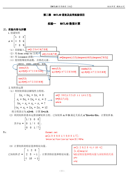
第二章 MATLAB 语言及应用实验项目实验一 MATLAB 数值计算三、实验内容与步骤1.创建矩阵⎥⎥⎥⎦⎤⎢⎢⎢⎣⎡=987654321a(1(2)用(3)用(42.矩阵的运算(1)利用矩阵除法解线性方程组。
⎪⎪⎩⎪⎪⎨⎧=+++=-+-=+++=+-12224732258232432143214321421x x x x x x x x x x x x x x x 将方程表示为AX=B ,计算X=A\B 。
(2)利用矩阵的基本运算求解矩阵方程。
已知矩阵A 和B 满足关系式A -1BA=6A+BA ,计算矩阵B 。
其中⎥⎥⎥⎦⎤⎢⎢⎢⎣⎡=7/10004/10003/1A ,Ps: format rata=[1/3 0 0;0 1/4 0;0 0 1/7];b=inv(a)*inv(inv(a)-eye(3))*6*a(3)计算矩阵的特征值和特征向量。
已知矩阵⎥⎥⎥⎦⎤⎢⎢⎢⎣⎡--=1104152021X ,计算其特征值和特征向量。
(4)Page:322利用数学函数进行矩阵运算。
已知传递函数G(s)=1/(2s+1),计算幅频特性Lw=-20lg(1)2(2w )和相频特性Fw=-arctan(2w),w 的范围为[0.01,10],按对数均匀分布。
3.多项式的运算(1)多项式的运算。
已知表达式G(x)=(x-4)(x+5)(x 2-6x+9),展开多项式形式,并计算当x 在[0,20]内变化时G(x)的值,计算出G(x)=0的根。
Page 324(2)多项式的拟合与插值。
将多项式G(x)=x 4-5x 3-17x 2+129x-180,当x 在[0,20]多项式的值上下加上随机数的偏差构成y1,对y1进行拟合。
对G(x)和y1分别进行插值,计算在5.5处的值。
Page 325 四、思考练习题1.使用logspace 函数创建0~4π的行向量,有20个元素,查看其元素分布情况。
Ps: logspace(log10(0),log10(4*pi),20) (2) sort(c,2) %顺序排列 3.1多项式1)f(x)=2x 2+3x+5x+8用向量表示该多项式,并计算f(10)值. 2)根据多项式的根[-0.5 -3+4i -3-4i]创建多项式。
matlab表达式转换为word公式

将Matlab 表达式转换为word 公式(1) Matlab 可以把公式表达式转换为Cfortran 格式,也可以转换为Latex 排版格式,由于Latex 公式的控制格式是纯文本的,因此任何表达式要转换为Latex 格式都是很简单的,Maple 、Mathematica 都提供了类似功能。
(2) MathType 6.0版提供了将Latex 转换为Mathtype 公式的功能,这意味着用Matlab/Mathematica/maple 计算出来的公式可以先转换为Latex ,然后再直接转换为MathType 公式。
方法:在MathType 要导入,先复制Latex 表达式,然后直接粘贴进来就可以看到公式了。
(3) MathType 还可以导出和导入为windows 图元文件emf 矢量图片格式gif ,这意味着如果你有一个公式是图片格式的,可以转换为这两种格式,然后用MathType 导入并编辑。
最后来一个Matlab 代码运算结果转换为MathType 公式的例子: syms x y;f=sin(x)*exp(y)+log(y)*cos(x);f=diff(diff(f,x,2),y,2) %输出matlab 公式形式fs=latex(f) %输出latex 公式形式f =-sin(x)*exp(y)+1/y^2*cos(x)fs =-\sin \left( x \right) {e^{y}}+{\frac {\cos \left( x \right) }{{y}^{2}}}在MathType 中选择转换选项后,把上面的代码直接复制进去就可以看到下面的公式了。
最后再做一些小修改,比如括号、下标,MATLAB 里没下标,括号有时也是多余。
()()2cos sin y x fs x e y =-+文章来源/blog/static/29562664200772354258481/。
MATLAB仿真与建模中常见问题与解决方法

MATLAB仿真与建模中常见问题与解决方法引言MATLAB作为一种功能强大的数学软件平台,被广泛应用于科学研究、工程设计等领域。
然而,在进行MATLAB仿真和建模过程中,常常会遇到一些问题和困惑。
本文将针对这些常见问题,提供一些解决方法和建议,帮助读者更好地应对挑战。
1. 数据处理问题在仿真和建模过程中,数据处理是一个常见的问题。
首先,当我们从实验中获得大量数据时,如何进行处理和分析就成为一个关键问题。
MATLAB提供了各种强大的数据处理函数,例如mean、std、histogram等,可以帮助我们对数据进行统计和可视化分析。
此外,MATLAB还提供了数据拟合函数和插值函数,可以对数据进行拟合和补全。
另一个常见的数据处理问题是数据噪声的处理。
在实际应用中,测量数据常常存在噪声,这会对仿真和建模结果产生影响。
为了解决这个问题,我们可以使用滤波器函数来降低噪声的影响。
MATLAB中常用的滤波器函数有移动平均滤波器和中值滤波器等。
2. 优化问题在一些实际应用中,我们需要对模型进行优化,以找到最优解。
MATLAB提供了一些优化算法和工具箱,可以帮助我们解决这个问题。
一种常见的优化算法是遗传算法,它模拟了自然界的进化过程,通过遗传操作来搜索最优解。
MATLAB中的Global Optimization Toolbox提供了遗传算法的实现。
此外,MATLAB还提供了其他优化算法,如线性规划、非线性规划和整数规划等。
通过选择合适的算法和设置适当的优化目标,我们可以得到满意的优化结果。
3. 建模问题在建模过程中,我们常常需要选择适当的模型和参数来描述系统。
这需要一定的经验和技巧。
MATLAB提供了一些建模工具和函数,可以帮助我们更好地处理这个问题。
首先,MATLAB中的Curve Fitting Toolbox提供了各种曲线拟合函数,如线性拟合、多项式拟合和非线性拟合等。
通过选择合适的模型和调整参数,我们可以将实验数据拟合成理想的曲线。
经典功率谱估计Welch法的MATLAB仿真分析

经典功率谱估计Welch法的MATLAB仿真分析杨晓明;晋玉剑;李永红【摘要】周期图法是经典功率谱估计中的一种基本方法,但是在实际应用中难以同时保证良好的分辨力和方差性能.因此本文以周期图法原理为切入点,对改进后的Welch算法进行研究,并借助MATLAB软件强大的信号处理与数值分析能力,对Welch算法的谱估计分辨力、方差等性能进行仿真分析.讨论了不同数据分段长度、不同窗函数类型等因素对算法性能产生的影响.仿真结果表明,Welch算法由于合理的引入数据分段和窗函数,得到了较好的方差性能以及分辨能力,但在对短数据进行功率谱估计时还有一定的局限性.【期刊名称】《电子测试》【年(卷),期】2011(000)007【总页数】4页(P101-104)【关键词】经典功率谱估计;周期图法;Welch法;MATLAB仿真【作者】杨晓明;晋玉剑;李永红【作者单位】中北大学,太原,030051;中北大学,太原,030051;中北大学,太原,030051【正文语种】中文【中图分类】TN911.720 引言在对平稳随机信号的频谱分析中,由于其不满足平方可积、非周期性等特点,只有应用功率谱估计(PSD)才能根据有限长信号估计出原信号的真实功率谱[1]。
文中通过分析经典功率谱周期图法的原理与所存在的缺陷,进而对改进后的Welch算法进行了讨论,并通过MATLAB软件进行仿真。
分析仿真曲线后得出结论,Welch算法通过数据分段和加窗,有效降低谱估计的方差,同时又不使分辨力遭到严重破坏,是一种有效的谱估计方法[2],仿真过程中也同时发现算法存在一定的局限性。
1 经典功率谱估计Welch算法经典谱估计是将数据工作区外的未知数据假设为零,相当于数据加窗。
它可以分为用随机序列求谱的自相关法和将序列直接用FFT求谱的直接法,以及改进后的Bartlett法和Welch法。
1.1 周期图法(直接法)周期图(Periodogram)的概念是在19世纪末由Schuster提出。
Matlab仿真波形转到Word以及FFT波形处理

仿真波形如何转到Word的文档一、仿真波形如何转到Word,及如何修改与标注坐标步骤如下:1、先从Matlab/Simulink中选出时钟Clock 以及To Workspace模块并连接起来,如下图1-1。
然后打开To Workspace,如下图1-2,接着设置参数:修改Variable name为t(可自己定义),Sample time为2e-4(可自己定义),Save format为Array。
图1-1图1-22、选择To Workspace接到需要的位置,比如要测A相电流,打开To Workspace,设置如下图1-3,同图1-2类似,只要修改Variable name为ia(可自己定义)。
注:Sample time必须与步骤1中的Sample time一致。
图1-33、步骤1、2完成后,开始仿真运行,仿真完成后,在Matlab命令行中输入plot(t,ia),然后单机Enter键确定后,便可显示如下图1-4所示的仿真波形。
图1-44、点击Edit,如下图1-5所示,然后选择Edit图标下的Axes Properties…,显示结果如下图6所示。
图1-5图1-65、在图1-6下方的方框内点击X Axis,选择X Label:输入t/s,即标注了横坐标时间t,单位为秒(s),如下图1-7所示。
然后可以修改X Limits参数,即横坐标范围。
图1-7同理设置Y Axis。
选择Y Label:输入i a/A,即标注了纵坐标电流i a,单位为安培(A)。
6、完成上述步骤后,选择Edit图标下的Copy Figure命令,如图1-8所示。
最后粘帖到Word中,得到所需a相电流波形i a如图1-9所示。
图1-8图1-9注:可以采用Edit 图标下的Axes Properties 中的grid 命令,会产生如下图1-10所示的效果。
当然还可以采用Subplot 等命令,将2、3个仿真波形放到一个图中对比显示。
MATLAB7.0使用详解-第19章 Word和Excel环境下
19.1.4 输出元胞的格式设置
读者应该看到图中显示的蓝色的结果同样被一个方括号包围,这 就是输出元胞。输出元胞可以包含各种类型的结果,用户可以使 用Notebook设置对话框(Notebook Options),对输出元胞的结 果各项属性进行设置。 用户可以选择菜单栏上的Notebook\Notebook Options选项,打开 设置对话框,如图所示。
19.1.5 Notebook菜单功能选项
关于Notebook菜单中的选项,前几小节已经陆续介绍了一些,读者首先仔 细浏览一下Notebook菜单栏的所有选项,如图所示。 本节将介绍其他重要选项的功能和使用方法。 1.定义“自初始化元胞”(Define AutoInit Cell) 2.定义“计算区”(Define Calc Zone) 3.定义“元胞组”(Define Cells) 4.元胞图形输出拨动控制开关设置(Toggle Graph Output for Cell) 5.元胞的循环运行(Evaluate Loop) 6.撤消元胞定义(Undefine Cells)
19.1.2 Notebook的启动及初始化
当Notebook的安装成功后,用户可以使用两种方法打开Notebook,一种是 在Word里启动,另一种方法是在MATLAB中启动。首先介绍在Word中启动的 方法。 (1)在Windows环境下打开Word。所得到的窗口是以默认模板Normal.dot 创建的。 (2)创建新的M-book。选择“文件”菜单中的“新建”选项,系统弹出 新建文档对话框。 (3)选择M-book模板。在弹出的模板选择对话框中选择M-book.dot模板。 (4)Notebook启动完成。系统生成一个新的Word文档,在标题栏多出了 Notebook菜单。
图像压缩编码中Walsh变换与DCT变换及其比较
图像压缩编码中Walsh变换与DCT变换及其比较龙清【期刊名称】《现代电子技术》【年(卷),期】2011(34)10【摘要】图像变换是图像处理的基础,是图像压缩的第一步.在图像压缩中,DCT变换因其变换效果好而被广泛采用,成为目前最常用的图像压缩变换方法,而Walsh变换还未被广泛采用.通过对这两种变换的算法分析以及Matlab仿真实验和峰值信噪比的对比,结果表明,Walsh变换在算法上比DCT简单,实现较为容易,其变换性能并不亚于DCT变换,在某些量化级上甚至还优于DCT变换,Walsh变换有着广泛的应用前景.%Image transform is the foundation of image processing and the first step of image compression coding. Because of its good effect in image transform, the DCT transform has been used widely, and has became the most common transform method in image compression coding. By analyzing the DCT transform and Walsh transform, and comparing the MATLAB simulation experiment with PSNR, the results show that the Walsh transform is not inferior to the DCT transform in performance, and in some quantitative level it is superior to the DCT transform. Besides, the Walsh transform is simpler than the DCT in algorithm. It can be used widely in future.【总页数】5页(P12-16)【作者】龙清【作者单位】重庆广播电视集团(总台),重庆401147【正文语种】中文【中图分类】TN919-34;TP391.41【相关文献】1.Walsh变换在彩色图像压缩编码中的应用 [J], 李钰;赵铁民2.一种基于分块DCT变换的嵌入式图像压缩编码算法 [J], 王延求3.基于DCT变换的图像压缩编码的MATLAB实现 [J], 彭干涛;禹峰;林嘉居4.H.264/AVC中的整数变换与DCT变换的比较 [J], 杜路泉;王泽勇;王黎;高晓蓉5.DCT变换图像压缩编码算法 [J], 王延求因版权原因,仅展示原文概要,查看原文内容请购买。
matlab的仿真流程总结
matlab的仿真流程总结下载温馨提示:该文档是我店铺精心编制而成,希望大家下载以后,能够帮助大家解决实际的问题。
文档下载后可定制随意修改,请根据实际需要进行相应的调整和使用,谢谢!并且,本店铺为大家提供各种各样类型的实用资料,如教育随笔、日记赏析、句子摘抄、古诗大全、经典美文、话题作文、工作总结、词语解析、文案摘录、其他资料等等,如想了解不同资料格式和写法,敬请关注!Download tips: This document is carefully compiled by theeditor. I hope that after you download them,they can help yousolve practical problems. The document can be customized andmodified after downloading,please adjust and use it according toactual needs, thank you!In addition, our shop provides you with various types ofpractical materials,such as educational essays, diaryappreciation,sentence excerpts,ancient poems,classic articles,topic composition,work summary,word parsing,copy excerpts,other materials and so on,want to know different data formats andwriting methods,please pay attention!1. 问题定义与分析明确仿真的目的和要解决的问题。
确定系统的输入、输出和关键参数。
walsh变换matlab仿真-word2003
Open walshhadamarddemo.m in the EditorRun in the Command WindowDiscrete Walsh-Hadamard Transform Contents•Introduction•Walsh (or Hadamard) Functions•Discrete Walsh-Hadamard Transform•Walsh-Transform Applications•ReferencesIntroductionThe Walsh-Hadamard transform (WHT) is a suboptimal, non-sinusoidal, orthogonal transformation that decomposes a signal into a set of orthogonal, rectangular waveforms called Walsh functions. The transformation has no multipliers and is real because the amplitude of Walsh (or Hadamard) functions has only two values, +1 or -1.WHTs are used in many different applications, such as power spectrum analysis, filtering, processing speech and medical signals, multiplexing and coding in communications, characterizing non-linear signals, solving non-linear differential equations, and logical design and analysis.This demo provides an overview of the Walsh-Hadamard transform and some of its properties by showcasing two applications, communications using spread spectrum and processing of ECG signals.Walsh (or Hadamard) FunctionsWalsh functions are rectangular or square waveforms with values of -1 or +1. An important characteristic of Walsh functions is sequency which is determined from the number of zero-crossings per unit time interval. Every Walsh function has a unique sequency value.Walsh functions can be generated in many ways (see [1]). Here we use the hadamard fu nction in MATLAB® to generate Walsh functions. Length eight Walsh functions are generated as follows.N = 8; % Length of Walsh (Hadamard) functionshadamardMatrix = hadamard(N)hadamardMatrix =1 1 1 1 1 1 1 11 -1 1 -1 1 -1 1 -11 1 -1 -1 1 1 -1 -11 -1 -1 1 1 -1 -1 11 1 1 1 -1 -1 -1 -11 -1 1 -1 -1 1 -1 11 1 -1 -1 -1 -1 1 11 -1 -1 1 -1 1 1 -1The rows (or columns) of the symmetric hadamardMatrix contain the Walsh functions. The Walsh functions in the matrix are not arranged in increasing order of their sequencies or number of zero-crossings (i.e. 'sequency order') but are arranged in 'Hadamard order'. The Walsh matrix, which contains the Walsh functions along the rows or columns in the increasing order of their sequencies is obtained by changing the index of the hadamardMatrix as follows.HadIdx = 0:N-1; % Hadamard indexM = log2(N)+1; % Number of bits to represent the indexEach column of the sequency index (in binary format) is given by the modulo-2 addition of columns of the bit-reversed Hadamard index (in binary format).binHadIdx = fliplr(dec2bin(HadIdx,M))-'0'; % Bit reversing of the binary indexbinSeqIdx = zeros(N,M-1); % Pre-allocate memoryfor k = M:-1:2% Binary sequency indexbinSeqIdx(:,k) = xor(binHadIdx(:,k),binHadIdx(:,k-1));endSeqIdx = binSeqIdx*pow2((M-1:-1:0)'); % Binary to integer sequency indexwalshMatrix = hadamardMatrix(SeqIdx+1,:) % 1-based indexing walshMatrix =1 1 1 1 1 1 1 11 1 1 1 -1 -1 -1 -11 1 -1 -1 -1 -1 1 11 1 -1 -1 1 1 -1 -11 -1 -1 1 1 -1 -1 11 -1 -1 1 -1 1 1 -11 -1 1 -1 -1 1 -1 11 -1 1 -1 1 -1 1 -1Discrete Walsh-Hadamard TransformThe forward and inverse Walsh transform pair for a signal x(t) of length N areFast algorithms, similar to the Cooley-Tukey algorithm, have been developed to implement the Walsh-Hadamard transform with complexityO(NlogN) (see [1] and [2]). Since the Walsh matrix is symmetric, both the forward and inverse transformations are identical operations except for the scaling factor of 1/N. The functions fwht and ifwht implement the forward and the inverse WHT respectively.Example 1 Perform WHT on the Walsh matrix. The expected result is an identity matrix because the rows (or columns) of the symmetric Walsh matrix contain the Walsh functions.y1 = fwht(walshMatrix) % Fast Walsh-Hadamard transform y1 =1 0 0 0 0 0 0 00 1 0 0 0 0 0 00 0 1 0 0 0 0 00 0 0 1 0 0 0 00 0 0 0 1 0 0 00 0 0 0 0 1 0 00 0 0 0 0 0 1 00 0 0 0 0 0 0 1Example 2Construct a discontinuous signal by scaling and adding arbitrary columns of the Hadamard matrix. This signal is formed using weighted Walsh functions, so the WHT should return non-zero values equal to the weights at the respective sequency indices. While evaluating the WHT, the ordering is specified as 'hadamard', because a Hadamard matrix (instead of the Walsh matrix) is used to obtain the Walsh functions.N = 8;H = hadamard(N); % Hadamard matrix% Construct a signal by adding a few weighted Walsh functionsx = 8.*H(1,:) + 12.*H(3,:) + 18.*H(5,:) + 10.*H(8,:);y = fwht(x,N,'hadamard')y =8 0 12 0 18 0 0 10WHT is a reversible transform and the original signal can be recovered perfectly using the inverse transform. The norm between the original signal and the signal obtained from inverse transformation equals zero, indicating perfect reconstruction.xHat = ifwht(y,N,'hadamard');norm(x-xHat)ans =The Walsh-Hadamard transform involves expansion using a set of rectangular waveforms, so it is useful in applications involving discontinuous signals that can be readily expressed in terms of Walsh functions. Below are two applications of Walsh-Hadamard transforms.Walsh-Transform ApplicationsECG signal processing Often, it is necessary to record electro-cardiogram (ECG) signals of patients at different instants of time. This results in a large amount of data, which needs to be stored for analysis, comparison, etc. at a later time. Walsh-Hadamard transform is suitable for compression of ECG signals because it offers advantages such as fast computation of Walsh-Hadamard coefficients, less required storage space since it suffices to store only those sequency coefficients with large magnitudes, and fast signal reconstruction.An ECG signal and its corresponding Walsh-Hadamard transform is evaluated and shown below.x1 = ecg(512); % Single ecg wavex = repmat(x1,1,8);x = x + 0.1.*randn(1,length(x)); % Noisy ecg signaly = fwht(x); % Fast Walsh-Hadamard transform figure('Color','white');subplot(2,1,1);plot(x);xlabel('Sample index');ylabel('Amplitude');title('ECG Signal');subplot(2,1,2);plot(abs(y))xlabel('Sequency index');ylabel('Magnitude');title('WHT Coefficients');As can be seen in the above plot, most of the signal energy is concentrated at lower sequency values. For investigation purposes, only the first 1024 coefficients are stored and used to reconstruct the original signal. Truncating the higher sequency coefficients also helps with noise suppression. The original and the reproduced signals are shown below.y(1025:length(x)) = 0; % Zeroing out the higher coefficients xHat = ifwht(y); % Signal reconstruction using inverse WHTfigure('Color','white');plot(x);hold onplot(xHat,'r');xlabel('Sample index');ylabel('ECG signal amplitude');legend('Original Signal','Reconstructed Signal');x=ecg(512);x1=repmat(x,1,8);x1=x1+0.1*randn(1,length(x1));figure('Color','white');y1=fft(x1);subplot(2,1,1)plot(abs(y1))y1(201:length(x1))=0;xhat=ifft(y1);plot(abs(xhat))x2 = ecg(512); % Single ecg wavex = repmat(x2,1,8);x = x + 0.1.*randn(1,length(x));plot(x)y1(1025:length(x1))=0;xhat=ifft(y1);plot(abs(xhat))The reproduced signal is very close to the original signal.To reconstruct the original signal, we stored only the first 1024 coefficients and the ECG signal length. This represents a compression ratio of approximately 4:1.req = [length(x) y(1:1024)];whos x reqName Size Bytes Class Attributesreq 1x1025 8200 doublex 1x4096 32768 doubleCommunication using Spread Spectrum Spread spectrum-based communication technologies, like CDMA, use Walsh codes (derived from Walsh functions) to spread message signals and WHT transforms to despread them. Since Walsh codes are orthogonal, any Walsh-encoded signal appears as random noise to a terminal unless that terminal uses the same code for encoding. Below we demonstrate the process of spreading, determining Walsh codes used for spreading, and despreading to recover the message signal.Two CDMA terminals spread their respective message signals using two different Walsh codes (also known as Hadamard codes) of length 64. The spread message signals are corrupted by a additive white Gaussian noise of variance 0.1.At the receiver (base station), signal processing is non-coherent and the received sequence of length N needs to be correlated with 2^N Walsh codewords to extract the Walsh codes used by the respective transmitters. This can be effectively done by transforming the received signals to sequency domain using the fast Walsh-Hadamard transform. Using the sequency location at a which a peak occurs, the correspondingWalsh-Hadamard code (or the Walsh function) used can be determined. The plot below shows that Walsh-Hadamard codes with sequency (with ordering = 'hadamard') 60 and 10 were used in the first and the second transmitter, respectively.load mess_rcvd_signals.matN = length(rcvdSig1);y1 = fwht(rcvdSig1,N,'hadamard');y2 = fwht(rcvdSig2,N,'hadamard');figure('Color','white');plot(0:63,y1,0:63,y2,'r');xlabel('Sequency index');ylabel('WHT of the Received Signals');title('Walsh-Hadamard Code Extraction');legend('WHT of Tx - 1 signal','WHT of Tx - 2 signal');Despreading (or decoding) to extract the message signal can be carried out in a straightforward manner by multiplying the received signals by the respective Walsh-hadamard codes generated using the hadamard function. (Note that the indexing in MATLAB® starts from 1, hence Walsh-Hadamard codes with sequency 60 and 10 are obtained from by selecting the columns (or rows) 61 and 11 in the Hadamard matrix.)N = 64;hadamardMatrix = hadamard(N);codeTx1 = hadamardMatrix(:,61); % Code used by transmitter 1 codeTx2 = hadamardMatrix(:,11); % Code used by transmitter 2The decoding operation to recover the original message signal isxHat1 = codeTx1 .* rcvdSig1; % Decoded signal at receiver 1 xHat2 = codeTx2 .* rcvdSig2; % Decoded signal at receiver 2The recovered message signals at the receiver side are shown below and superimposed with the original signals for comparison.subplot(2,1,1);plot(x1);hold onplot(xHat1,'r');legend('Original Message','Reconstructed Message','Location','Best'); xlabel('Sample index');ylabel('Message signal amplitude');subplot(2,1,2);plot(x2);hold onplot(xHat2,'r');legend('Original Message','Reconstructed Message','Location','Best'); xlabel('Sample index');ylabel('Message signal amplitude');References1.K.G. Beauchamp, Applications of Walsh and Related Functions - Withan Introduction to Sequency Theory, Academic Press, 19842.T. Beer, Walsh Transforms, American Journal of Physics, Vol. 49,Issue 5, May 1981Copyright 2008-2010 The MathWorks, Inc.Published with MATLAB® 7.13MATLAB and Simulink are registered trademarks of The MathWorks, Inc. Please see aaamathworksaaa/trademarks for a list of other trademarks owned by The MathWorks, Inc. Other product or brand names are trademarks or registered trademarks of their respective owners.[文档可能无法思考全面,请浏览后下载,另外祝您生活愉快,工作顺利,万事如意!]11 / 11。
利用MATLAB仿真软件系统结合双线性变换法设计一个数字巴特沃斯高通IIR滤波器.
摘要Matlab是一个矩阵设计平台,传统数字滤波器设计需要大量的计算,但是利用Matlab可以快速实现滤波器的设计与仿真,而且频谱分析功能强大,在数字信号处理中发挥了巨大的作用。
本次实验中,用双线性不变法设计高通巴特沃斯IIR数字滤波器,介绍了设计步骤,然后在Matlab环境下进行了仿真与调试,实现了设计目标。
关键词:Matlab 数字滤波器双线性变换法 IIR摘要Matlab是一个矩阵设计平台,传统数字滤波器设计需要大量的计算,但是利用Matlab可以快速实现滤波器的设计与仿真,而且频谱分析功能强大,在数字信号处理中发挥了巨大的作用。
本次实验中,用双线性不变法设计高通巴特沃斯IIR数字滤波器,介绍了设计步骤,然后在Matlab环境下进行了仿真与调试,实现了设计目标。
关键词:Matlab 数字滤波器双线性变换法 IIR()Nj G 2c 2Ωj Ωj 11Ω⎪⎪⎭⎫ ⎝⎛+=摘要Matlab 是一个矩阵设计平台,传统数字滤波器设计需要大量的计算,但是利用Matlab 可以快速实现滤波器的设计与仿真,而且频谱分析功能强大,在数字信号处理中发挥了巨大的作用。
本次实验中,用双线性不变法设计高通巴特沃斯IIR 数字滤波器,介绍了设计步骤,然后在Matlab 环境下进行了仿真。
关键词:Matlab 数字滤波器 双线性变换法1设计要求和说明利用MATLAB 仿真软件系统结合双线性变换法设计一个数字巴特沃斯高通IIR 滤波器。
MATLAB 工具箱为滤波器的设计应用提供了丰富而简便的方法,使原来的非常繁琐复杂的程序设计变成简单的程序调用。
1.1 设计原理滤波器,顾名思义,就是对系统输入信号进行滤波。
那个数字滤波器的数学运算通常用两种方法来表示。
一种是频域法,即利用FFT 快速运算办法对输入信号进行离散傅里叶变换,分析其频谱,然后根据所希望的频率特性进行滤波,再利用傅里叶反变换来输出出时域信号。
N 阶低通巴特沃斯滤波器的特性为:其中,Ωc 为通带宽度,即截止频率。
- 1、下载文档前请自行甄别文档内容的完整性,平台不提供额外的编辑、内容补充、找答案等附加服务。
- 2、"仅部分预览"的文档,不可在线预览部分如存在完整性等问题,可反馈申请退款(可完整预览的文档不适用该条件!)。
- 3、如文档侵犯您的权益,请联系客服反馈,我们会尽快为您处理(人工客服工作时间:9:00-18:30)。
Open walshhadamarddemo.m in the EditorRun in the Command WindowDiscrete Walsh-Hadamard Transform Contents•Introduction•Walsh (or Hadamard) Functions•Discrete Walsh-Hadamard Transform•Walsh-Transform Applications•ReferencesIntroductionThe Walsh-Hadamard transform (WHT) is a suboptimal, non-sinusoidal, orthogonal transformation that decomposes a signal into a set of orthogonal, rectangular waveforms called Walsh functions. The transformation has no multipliers and is real because the amplitude of Walsh (or Hadamard) functions has only two values, +1 or -1.WHTs are used in many different applications, such as power spectrum analysis, filtering, processing speech and medical signals, multiplexing and coding in communications, characterizing non-linear signals, solving non-linear differential equations, and logical design and analysis.This demo provides an overview of the Walsh-Hadamard transform and some of its properties by showcasing two applications, communications using spread spectrum and processing of ECG signals.Walsh (or Hadamard) FunctionsWalsh functions are rectangular or square waveforms with values of -1 or +1. An important characteristic of Walsh functions is sequency which is determined from the number of zero-crossings per unit time interval. Every Walsh function has a unique sequency value.Walsh functions can be generated in many ways (see [1]). Here we use the hadamard function in MATLAB® to generate Walsh functions. Length eight Walsh functions are generated as follows.N = 8; % Length of Walsh (Hadamard) functionshadamardMatrix = hadamard(N)hadamardMatrix =1 1 1 1 1 1 1 11 -1 1 -1 1 -1 1 -11 1 -1 -1 1 1 -1 -11 -1 -1 1 1 -1 -1 11 1 1 1 -1 -1 -1 -11 -1 1 -1 -1 1 -1 11 1 -1 -1 -1 -1 1 11 -1 -1 1 -1 1 1 -1The rows (or columns) of the symmetric hadamardMatrix contain the Walsh functions. The Walsh functions in the matrix are not arranged in increasing order of their sequencies or number of zero-crossings (i.e. 'sequency order') but are arranged in 'Hadamard order'. The Walsh matrix, which contains the Walsh functions along the rows or columns in the increasing order of their sequencies is obtained by changing the index of the hadamardMatrix as follows.HadIdx = 0:N-1; % Hadamard indexM = log2(N)+1; % Number of bits to represent the indexEach column of the sequency index (in binary format) is given by the modulo-2 addition of columns of the bit-reversed Hadamard index (in binary format).binHadIdx = fliplr(dec2bin(HadIdx,M))-'0'; % Bit reversing of the binary indexbinSeqIdx = zeros(N,M-1); % Pre-allocate memoryfor k = M:-1:2% Binary sequency indexbinSeqIdx(:,k) = xor(binHadIdx(:,k),binHadIdx(:,k-1));endSeqIdx = binSeqIdx*pow2((M-1:-1:0)'); % Binary to integer sequency indexwalshMatrix = hadamardMatrix(SeqIdx+1,:) % 1-based indexing walshMatrix =1 1 1 1 1 1 1 11 1 1 1 -1 -1 -1 -11 1 -1 -1 -1 -1 1 11 1 -1 -1 1 1 -1 -11 -1 -1 1 1 -1 -1 11 -1 -1 1 -1 1 1 -11 -1 1 -1 -1 1 -1 11 -1 1 -1 1 -1 1 -1Discrete Walsh-Hadamard TransformThe forward and inverse Walsh transform pair for a signal x(t) of length N areFast algorithms, similar to the Cooley-Tukey algorithm, have been developed to implement the Walsh-Hadamard transform with complexityO(NlogN) (see [1] and [2]). Since the Walsh matrix is symmetric, both the forward and inverse transformations are identical operations except for the scaling factor of 1/N. The functions fwht and ifwht implement the forward and the inverse WHT respectively.Example 1 Perform WHT on the Walsh matrix. The expected result is an identity matrix because the rows (or columns) of the symmetric Walsh matrix contain the Walsh functions.y1 = fwht(walshMatrix) % Fast Walsh-Hadamard transform y1 =1 0 0 0 0 0 0 00 1 0 0 0 0 0 00 0 1 0 0 0 0 00 0 0 1 0 0 0 00 0 0 0 1 0 0 00 0 0 0 0 1 0 00 0 0 0 0 0 1 00 0 0 0 0 0 0 1Example 2Construct a discontinuous signal by scaling and adding arbitrary columns of the Hadamard matrix. This signal is formed using weighted Walsh functions, so the WHT should return non-zero values equal to the weights at the respective sequency indices. While evaluating the WHT, the ordering is specified as 'hadamard', because a Hadamard matrix (instead of the Walsh matrix) is used to obtain the Walsh functions.N = 8;H = hadamard(N); % Hadamard matrix% Construct a signal by adding a few weighted Walsh functionsx = 8.*H(1,:) + 12.*H(3,:) + 18.*H(5,:) + 10.*H(8,:);y = fwht(x,N,'hadamard')y =8 0 12 0 18 0 0 10WHT is a reversible transform and the original signal can be recovered perfectly using the inverse transform. The norm between the original signal and the signal obtained from inverse transformation equals zero, indicating perfect reconstruction.xHat = ifwht(y,N,'hadamard');norm(x-xHat)ans =The Walsh-Hadamard transform involves expansion using a set of rectangular waveforms, so it is useful in applications involving discontinuous signals that can be readily expressed in terms of Walsh functions. Below are two applications of Walsh-Hadamard transforms.Walsh-Transform ApplicationsECG signal processing Often, it is necessary to record electro-cardiogram (ECG) signals of patients at different instants of time. This results in a large amount of data, which needs to be stored for analysis, comparison, etc. at a later time. Walsh-Hadamard transform is suitable for compression of ECG signals because it offers advantages such as fast computation of Walsh-Hadamard coefficients, less required storage space since it suffices to store only those sequency coefficients with large magnitudes, and fast signal reconstruction.An ECG signal and its corresponding Walsh-Hadamard transform is evaluated and shown below.x1 = ecg(512); % Single ecg wavex = repmat(x1,1,8);x = x + 0.1.*randn(1,length(x)); % Noisy ecg signaly = fwht(x); % Fast Walsh-Hadamard transform figure('Color','white');subplot(2,1,1);plot(x);xlabel('Sample index');ylabel('Amplitude');title('ECG Signal');subplot(2,1,2);plot(abs(y))xlabel('Sequency index');ylabel('Magnitude');title('WHT Coefficients');As can be seen in the above plot, most of the signal energy is concentrated at lower sequency values. For investigation purposes, only the first 1024 coefficients are stored and used to reconstruct the original signal.Truncating the higher sequency coefficients also helps with noise suppression. The original and the reproduced signals are shown below.y(1025:length(x)) = 0; % Zeroing out the higher coefficients xHat = ifwht(y); % Signal reconstruction using inverse WHTfigure('Color','white');plot(x);hold onplot(xHat,'r');xlabel('Sample index');ylabel('ECG signal amplitude');legend('Original Signal','Reconstructed Signal');x=ecg(512);x1=repmat(x,1,8);x1=x1+0.1*randn(1,length(x1));figure('Color','white');y1=fft(x1);subplot(2,1,1)plot(abs(y1))y1(201:length(x1))=0;xhat=ifft(y1);plot(abs(xhat))x2 = ecg(512); % Single ecg wavex = repmat(x2,1,8);x = x + 0.1.*randn(1,length(x));plot(x)y1(1025:length(x1))=0;xhat=ifft(y1);plot(abs(xhat))The reproduced signal is very close to the original signal.To reconstruct the original signal, we stored only the first 1024 coefficients and the ECG signal length. This represents a compression ratio of approximately 4:1.req = [length(x) y(1:1024)];whos x reqName Size Bytes Class Attributesreq 1x1025 8200 doublex 1x4096 32768 doubleCommunication using Spread Spectrum Spread spectrum-based communication technologies, like CDMA, use Walsh codes (derived from Walsh functions) to spread message signals and WHT transforms to despread them. Since Walsh codes are orthogonal, any Walsh-encoded signal appears as random noise to a terminal unless that terminal uses the same code for encoding. Below we demonstrate the process of spreading, determining Walsh codes used for spreading, and despreading to recover the message signal.Two CDMA terminals spread their respective message signals using two different Walsh codes (also known as Hadamard codes) of length 64. The spread message signals are corrupted by a additive white Gaussian noise of variance 0.1.At the receiver (base station), signal processing is non-coherent and the received sequence of length N needs to be correlated with 2^N Walsh codewords to extract the Walsh codes used by the respective transmitters. This can be effectively done by transforming the received signals to sequency domain using the fast Walsh-Hadamard transform. Using the sequency location at a which a peak occurs, the correspondingWalsh-Hadamard code (or the Walsh function) used can be determined. The plot below shows that Walsh-Hadamard codes with sequency (with ordering = 'hadamard') 60 and 10 were used in the first and the second transmitter, respectively.load mess_rcvd_signals.matN = length(rcvdSig1);y1 = fwht(rcvdSig1,N,'hadamard');y2 = fwht(rcvdSig2,N,'hadamard');figure('Color','white');plot(0:63,y1,0:63,y2,'r');xlabel('Sequency index');ylabel('WHT of the Received Signals');title('Walsh-Hadamard Code Extraction');legend('WHT of Tx - 1 signal','WHT of Tx - 2 signal');Despreading (or decoding) to extract the message signal can be carried out in a straightforward manner by multiplying the received signals by the respective Walsh-hadamard codes generated using the hadamard function. (Note that the indexing in MATLAB® starts from 1, hence Walsh-Hadamard codes with sequency 60 and 10 are obtained from by selecting the columns (or rows) 61 and 11 in the Hadamard matrix.)N = 64;hadamardMatrix = hadamard(N);codeTx1 = hadamardMatrix(:,61); % Code used by transmitter 1 codeTx2 = hadamardMatrix(:,11); % Code used by transmitter 2The decoding operation to recover the original message signal isxHat1 = codeTx1 .* rcvdSig1; % Decoded signal at receiver 1 xHat2 = codeTx2 .* rcvdSig2; % Decoded signal at receiver 2The recovered message signals at the receiver side are shown below and superimposed with the original signals for comparison.subplot(2,1,1);plot(x1);hold onplot(xHat1,'r');legend('Original Message','Reconstructed Message','Location','Best'); xlabel('Sample index');ylabel('Message signal amplitude');subplot(2,1,2);plot(x2);hold onplot(xHat2,'r');legend('Original Message','Reconstructed Message','Location','Best'); xlabel('Sample index');ylabel('Message signal amplitude');References1.K.G. Beauchamp, Applications of Walsh and Related Functions - Withan Introduction to Sequency Theory, Academic Press, 19842.T. Beer, Walsh Transforms, American Journal of Physics, Vol. 49,Issue 5, May 1981Copyright 2008-2010 The MathWorks, Inc.Published with MATLAB® 7.13MATLAB and Simulink are registered trademarks of The MathWorks, Inc. Please see /trademarks for a list of other trademarks owned by The MathWorks, Inc. Other product or brand names are trademarks or registered trademarks of their respective owners.。