外文资料翻译--应用坐标测量机的机器人运动学姿态的标定翻译-精品
Robots机器人 中英文翻译
RobotsA robot is an automatically controlled, reprogrammable, multipurpose, mani pulating machine with several reprogrammable axes, which may be either fixed in place or mobile for use in industrial automation applications.The key words are reprogrammable and multipurpose because most single-purpose machines do not meet these two requirements.The term”reprogrammabl e” implies two things:The robot operates according to a written program can b e rewritten to accomdate a variety of manufacturing tasks. The term “multipurp ose” means that the robot can perform many different functions, depending on the program and tooling currently in use.Over the past two decades,the robot has been introduced into industry to perform many monotonous and often unsafe operations. Because robots can per form certain basic tasks more quickly and accurately than humans, they are bei ng increasingly used in various manufacturing industries.Structures of RobotsThe typical structure of industrial robots consists of 4 major components: the manipulator, the end effector, the power supply and control syterm.The manipulator is a mechanical unite that provides motions similar to those of a human arm. It often has a shoulder joint,an elbow and a wrist. It can rotate or slide, strech out and withdraw in every possible direction with certain flexibility.The basic mechanical configurations of the robot manipulator are categorized as Cartesian, cylindrical, spherical and articulated.A robot with a Cartesian geometry can move its gripper to any position within the cube or rectangle defined as its working volum.Cylindrical coordinate robots can move the gripper within a volum that is described by a cylinder. The cylindrical coordinate robot is positioned in the work area by two linear movements in the X and Y directions and one angular rotation about the Z axis.Spherical arm geometry robots have an irregular work envelop. This type of robot has two main variants,vertically articulated and horizontally articulated.The end effector attaches itself to the end of the robot wrist, also called end-of-arm tooling.It is the device intended for performing the designed operations as a human hand can.End effectors are generally custom-made to meet special handling requirements. Mechanical grippers are the most commonly used and are equipped with two or more fingers.The selection of an appropriate end effector for a special application depends on such factors as the payload, enviyonment,reliability,and cost.The power supply is the actuator for moving the robot arm, controlling the joints and operating the end effector. The basic type of power sources include electrical,pneumatic, and hydraulic. Each source of energy and each type of motor has its own characteristics, advantages and limitations. An ac-powered motor or dc-powered motor may be used depending on the system design and applications. These motors convert electrical energy into mechanical energy to power the robot.Most new robots use electrical power supply. Pneumatic actuators have been used for high speed. Nonservo robots and are often used for powering tooling such as grippers. Hydraulic actuators have been used for heavier lift systems, typically where accuracy was not also requied.The contro system is the communications and information-processing system that gives commands for the movements of the robot. It is the brain of the robot; it sends signals to the power source to move the robot arm to a specific position and to the end effector.It is also the nerves of the robot; it is reprogrammable to send out sequences of instructions for all movements and actions to be taken by the robot.A open-loop controller is the simplest for of the control system, which controls the robot only by foolowing the predetermined step-by-step instructions.This system dose not have a self-correcting capability.A close-loop control system use feedback sensors to produce signals that reflct the current states of the controed objects. By comparing those feedback signals with the values set by the programmer, the close-loop controller can conduct the robot to move to the precise position and assume the desired attitude, and the end effector can perform with very high accuracy as the close-loop control system can minimize the discrepancy between the controlled object and the predetermined references.Classification of RobotIndustrial robots vary widely in size,shape, number of axes,degrees of freedom, and design configuration. Each factor influence the dimensions of the robot’s working envelop or the volume of space within which it can move and perform its designated task. A broader classification of robots can been described as below.Fixed-and Variable-Sequence Robots. The fixed-sequence robot (also called a pick-and place robot) is programmed for a specific sequence of operations. Its movements are form point to point, and the cycle is repeated continuously.The variable-sequence robot can be programmed for a specific sequence of operations but can be programmed to perform another sequence of operation.Playback Robot. An operator leads or walks the playback robot and its end effector through the desired path. The robot memorizes and records the path and sequence of motions and can repeat them continually without any further action or guidance by the operator.Numerically Controlled Robot. The numerically controlled robot is programmed and operated much like a numerically controlled machine. The robot is servocontrolled by digital data, and its sequence of movements can be changed with relative ease.Intelligent Robot. The intelligent robot is capable of performing some of the functions and tasks carried out by huanbeings.It is equipped with a variety of sensors with visual and tactile capabilities.Robot ApplicationsThe robot is a very special type of productin tool; as a result, the applications in which robots are used are quite broad. These applications can be grouped into three categories: material processing, material handling and assembly.In material processing, robots use tools to process the raw material. For example, the robot tools could include a drill and the robot would be able to perfor drilling operaytions on raw material.Material handling consists of the loading, unloading, and transferring of workpieces in manufacturing facilities. These operations can be performed relatively and repeatedly with robots, thereby improving quality and scrap losses.Assembly is another large application area for using robotics. An automatic assembly system can incorporate automatic testing, robot automation and mechanical handling for reducing labor costs, increasing output and eliminating manual handling concers.机器人机器人是一种自动控制的、可重复编程的、多功能的、由几个可重复编程的坐标系来操纵机器的装置,它可以被固定在某地,还可以是移动的以在工业自动化工厂中使用。
机械外文翻译外文文献英文文献机械臂动力学与控制的研究

外文出处:Ellekilde, L. -., & Christensen, H. I. (2009). Control of mobile manipulator using the dynamical systems approach. Robotics and Automation, Icra 09, IEEE International Conference on (pp.1370 - 1376). IEEE.机械臂动力学与控制的研究拉斯彼得Ellekilde摘要操作器和移动平台的组合提供了一种可用于广泛应用程序高效灵活的操作系统,特别是在服务性机器人领域。
在机械臂众多挑战中其中之一是确保机器人在潜在的动态环境中安全工作控制系统的设计。
在本文中,我们将介绍移动机械臂用动力学系统方法被控制的使用方法。
该方法是一种二级方法, 是使用竞争动力学对于统筹协调优化移动平台以及较低层次的融合避障和目标捕获行为的方法。
I介绍在过去的几十年里大多数机器人的研究主要关注在移动平台或操作系统,并且在这两个领域取得了许多可喜的成绩。
今天的新挑战之一是将这两个领域组合在一起形成具有高效移动和有能力操作环境的系统。
特别是服务性机器人将会在这一方面系统需求的增加。
大多数西方国家的人口统计数量显示需要照顾的老人在不断增加,尽管将有很少的工作实际的支持他们。
这就需要增强服务业的自动化程度,因此机器人能够在室内动态环境中安全的工作是最基本的。
图、1 一台由赛格威RMP200和轻重量型库卡机器人组成的平台这项工作平台用于如图1所示,是由一个Segway与一家机器人制造商制造的RMP200轻机器人。
其有一个相对较小的轨迹和高机动性能的平台使它适应在室内环境移动。
库卡工业机器人具有较长的长臂和高有效载荷比自身的重量,从而使其适合移动操作。
当控制移动机械臂系统时,有一个选择是是否考虑一个或两个系统的实体。
在参考文献[1]和[2]中是根据雅可比理论将机械手末端和移动平台结合在一起形成一个单一的控制系统。
翻译中文
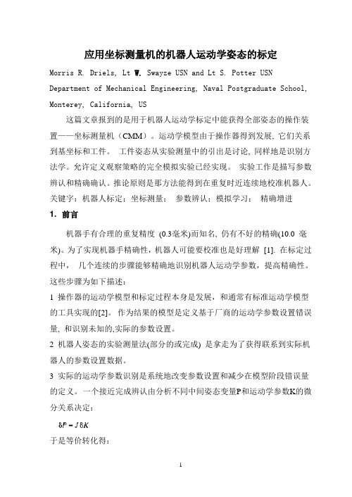
应用坐标测量机的机器人运动学姿态的标定Morris R. Driels, Lt W. Swayze USN and Lt S. Potter USN Department of Mechanical Engineering, Naval Postgraduate School, Monterey, California, US这篇文章报到的是用于机器人运动学标定中能获得全部姿态的操作装置——坐标测量机(CMM)。
运动学模型由于操作器得到发展, 它们关系到基坐标和工件。
工件姿态从实验测量中的引出是讨论, 同样地是识别方法学。
允许定义观察策略的完全模拟实验已经实现。
实验工作是描写参数辨认和精确确认。
推论原则是那方法能得到在重复时近连续地校准机器人。
关键字:机器人标定;坐标测量;参数辨认;模拟学习;精确增进1. 前言机器手有合理的重复精度(0.3毫米)而知名, 仍有不好的精确(10.0 毫米)。
为了实现机器手精确性,机器人可能要校准也是好理解[1]. 在标定过程中,几个连续的步骤能够精确地识别机器人运动学参数,提高精确性。
这些步骤为如下描述:1 操作器的运动学模型和标定过程本身是发展,和通常有标准运动学模型的工具实现的[2]。
作为结果的模型是定义基于厂商的运动学参数设置错误量, 和识别未知的,实际的参数设置。
2 机器人姿态的实验测量法(部分的或完成) 是拿走为了获得联系到实际机器人的参数设置数据。
3 实际的运动学参数识别是系统地改变参数设置和减少在模型阶段错误量的定义。
一个接近完成辨认由分析不同中间姿态变量P和运动学参数K的微分关系决定:于是等价转化得:两者择一, 问题可以看成为多维的优化问题,这是为了减少一些定义的错误功能到零点,运动学参数设置被改变。
这是标准优化问题和可能解决用的众所周知的[3] 方法。
4 最后一步是机械手控制中的机器人运动学识别和在学习之下的硬件系统的详细资料。
包含实验数据的这张纸用于标度过程。
机械手臂应用领域的外文文献以及翻译

机械手臂应用领域的外文文献以及翻译1. Introduction机械手臂是一种用于执行各种任务的自动化设备,其应用领域广泛。
本文档提供了一些关于机械手臂应用领域的外文文献,并附有简要的翻译。
2. 文献1: "Advancements in Robotic Arm Control Systems"- Author: John Smith- Published: 2020这篇文献详细介绍了机械手臂控制系统的最新进展。
作者讨论了各种控制算法、传感器和执行器的应用,以提高机械手臂的性能和精确度。
3. 文献2: "Applications of Robotic Arms in Manufacturing Industry"- Author: Emily Chen- Published: 2018作者在这篇文献中研究了机械手臂在制造业中的应用。
她列举了多个实例,包括机械手臂在装配、焊接和搬运等任务中的应用,以及通过使用机械手臂能够提高生产效率和质量的案例。
4. 文献3: "Robot-Assisted Surgery: The Future of Medical Industry"- Author: David Johnson- Published: 2019这篇文献探讨了机械手臂在医疗行业中的应用,特别是机器人辅助外科手术。
作者解释了机械手臂在手术过程中的优势,包括更小的切口、更高的精确度和减少术后恢复时间等方面。
5. 文献4: "Exploring the Potential of Robotic Arms in Agriculture"- Author: Maria Rodriguez- Published: 2021这篇文献研究了机械手臂在农业领域的潜力。
作者探讨了机械手臂在种植、收割和除草等农业任务中的应用,以及如何通过机械化技术改善农业生产的效率和可持续性。
人形机器人中英文对照外文翻译文献
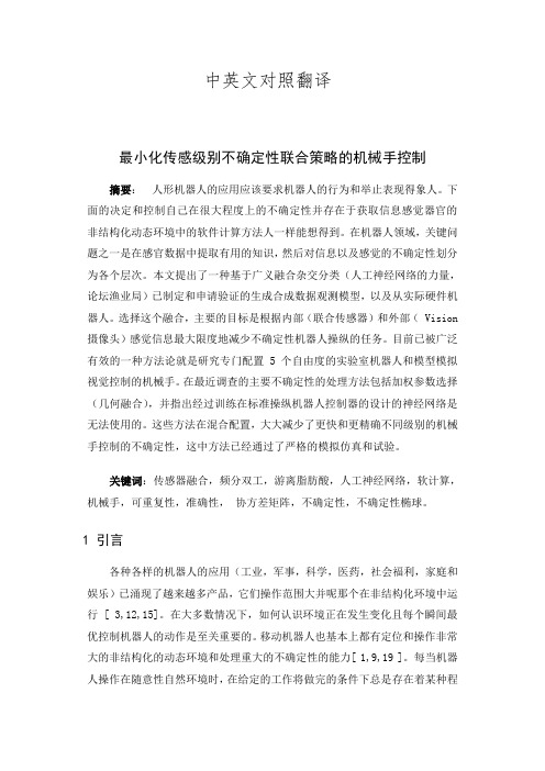
中英文对照翻译最小化传感级别不确定性联合策略的机械手控制摘要:人形机器人的应用应该要求机器人的行为和举止表现得象人。
下面的决定和控制自己在很大程度上的不确定性并存在于获取信息感觉器官的非结构化动态环境中的软件计算方法人一样能想得到。
在机器人领域,关键问题之一是在感官数据中提取有用的知识,然后对信息以及感觉的不确定性划分为各个层次。
本文提出了一种基于广义融合杂交分类(人工神经网络的力量,论坛渔业局)已制定和申请验证的生成合成数据观测模型,以及从实际硬件机器人。
选择这个融合,主要的目标是根据内部(联合传感器)和外部( Vision 摄像头)感觉信息最大限度地减少不确定性机器人操纵的任务。
目前已被广泛有效的一种方法论就是研究专门配置5个自由度的实验室机器人和模型模拟视觉控制的机械手。
在最近调查的主要不确定性的处理方法包括加权参数选择(几何融合),并指出经过训练在标准操纵机器人控制器的设计的神经网络是无法使用的。
这些方法在混合配置,大大减少了更快和更精确不同级别的机械手控制的不确定性,这中方法已经通过了严格的模拟仿真和试验。
关键词:传感器融合,频分双工,游离脂肪酸,人工神经网络,软计算,机械手,可重复性,准确性,协方差矩阵,不确定性,不确定性椭球。
1 引言各种各样的机器人的应用(工业,军事,科学,医药,社会福利,家庭和娱乐)已涌现了越来越多产品,它们操作范围大并呢那个在非结构化环境中运行 [ 3,12,15]。
在大多数情况下,如何认识环境正在发生变化且每个瞬间最优控制机器人的动作是至关重要的。
移动机器人也基本上都有定位和操作非常大的非结构化的动态环境和处理重大的不确定性的能力[ 1,9,19 ]。
每当机器人操作在随意性自然环境时,在给定的工作将做完的条件下总是存在着某种程度的不确定性。
这些条件可能,有时不同当给定的操作正在执行的时候。
导致这种不确定性的主要的原因是来自机器人的运动参数和各种确定任务信息的差异所引起的。
机器人技术的发展论文中英文对照资料外文翻译文献

机器人技术的发展论文中英文对照资料外文翻译文献摘要随着科技的不断发展,机器人技术在各个领域得到了广泛的应用。
本文翻译了几篇关于机器人技术的发展的文献,这些文献包括中文和英文内容。
其中,有关于机器人对人类生活的影响的讨论,也有机器人在工业、医疗等领域中的应用。
这些文献为大家提供了对机器人技术的深入了解,对于有关机器人技术的研究具有一定的参考价值。
正文中文文献机器人与人类生活随着机器人技术的不断发展,机器人已经开始逐渐进入人们的日常生活。
机器人从一开始的只能执行简单的任务,到现在已经能够和人类进行交互,甚至是取代人类在某些领域的工作。
随着机器人不断普及,对于机器人技术的伦理问题也越来越引人注目。
例如,机器人将如何与人类共存?机器人将如何对人类的生活产生影响?这些问题都亟待解决。
工业领域中的机器人工业领域是机器人技术得到广泛应用的领域之一。
机器人在工业生产中的应用不仅可以提高生产效率,还能减少人工操作对环境造成的影响。
目前,工业机器人已经能够完成许多需要人脑思考的任务,例如对产品进行分类、贴标签等。
随着机器人技术的不断发展,相信未来机器人在工业领域中的应用也会越来越广泛。
医疗领域中的机器人医疗领域是机器人技术应用的另一个重要领域。
机器人在医疗中的应用包括手术机器人、护理机器人等。
手术机器人可以进行精细的手术操作,并且可以通过微创手术减少患者的痛苦。
护理机器人可以为需要护理的人提供便利和帮助,减轻护理人员的负担。
这些机器人的出现,不仅提高了医疗领域的工作效率,还帮助了许多需要医疗服务的人。
英文文献Advances in Robotics TechnologyThis article reviews the recent advances in robotics technology. One of the biggest usages of robots is in the industrial sector, where the use in manufacturing process yields benefits such as increased efficiency and reduced costs. There are also a variety of robots for medical purposes, such as surgery and rehabilitation. In addition, robots are being used in the military and exploration of hostile environments to reduce risk to human life. The article concludes that robotics technology will continue to evolve and transform various industries with the potential to improve efficiency and reduce human error.Social Interaction with Robots结论本文翻译了关于机器人技术发展的中英文文献,并提供了机器人对人类生活的影响,机器人在工业、医疗中的应用等信息。
机器人外文翻译外文翻译、中英文翻译、外文文献翻译

外文翻译机器人The robot性质: □毕业设计□毕业论文教学院:机电工程学院系别:机械设计制造及其自动化学生学号:学生姓名:专业班级:指导教师:职称:起止日期:机器人1.机器人的作用机器人是高级整合控制论、机械电子、计算机、材料和仿生学的产物。
在工业、医学、农业、建筑业甚至军事等领域中均有重要用途。
现在,国际上对机器人的概念已经逐渐趋近一致。
一般说来,人们都可以接受这种说法,即机器人是靠自身动力和控制能力来实现各种功能的一种机器。
联合国标准化组织采纳了美国机器人协会给机器人下的定义:“一种可编程和多功能的,用来搬运材料、零件、工具的操作机;或是为了执行不同的任务而具有可改变和可编程动作的专门系统。
2.能力评价标准机器人能力的评价标准包括:智能,指感觉和感知,包括记忆、运算、比较、鉴别、判断、决策、学习和逻辑推理等;机能,指变通性、通用性或空间占有性等;物理能,指力、速度、连续运行能力、可靠性、联用性、寿命等。
因此,可以说机器人是具有生物功能的三维空间坐标机器。
3.机器人的组成机器人一般由执行机构、驱动装置、检测装置和控制系统等组成。
执行机构即机器人本体,其臂部一般采用空间开链连杆机构,其中的运动副(转动副或移动副)常称为关节,关节个数通常即为机器人的自由度数。
根据关节配置型式和运动坐标形式的不同,机器人执行机构可分为直角坐标式、圆柱坐标式、极坐标式和关节坐标式等类型。
出于拟人化的考虑,常将机器人本体的有关部位分别称为基座、腰部、臂部、腕部、手部(夹持器或末端执行器)和行走部(对于移动机器人)等。
驱动装置是驱使执行机构运动的机构,按照控制系统发出的指令信号,借助于动力元件使机器人进行动作。
它输入的是电信号,输出的是线、角位移量。
机器人使用的驱动装置主要是电力驱动装置,如步进电机、伺服电机等,此外也有采用液压、气动等驱动装置。
检测装置的作用是实时检测机器人的运动及工作情况,根据需要反馈给控制系统,与设定信息进行比较后,对执行机构进行调整,以保证机器人的动作符合预定的要求。
一个有关移动机器人定位的视觉传感器模型外文文献翻译、中英文翻译

XX设计(XX)外文资料翻译A Visual-Sensor Model for Mobile Robot Localisation Matthias Fichtner Axel Gro_mannArti_cial Intelligence InstituteDepartment of Computer ScienceTechnische Universit•at DresdenTechnical Report WV-03-03/CL-2003-02AbstractWe present a probabilistic sensor model for camera-pose estimation in hallways and cluttered o_ce environments. The model is based on the comparison of features obtained from a given 3D geometrical model of the environment with features present in the camera image. The techniques involved are simpler than state-of-the-art photogrammetric approaches. This allows the model to be used in probabilistic robot localisation methods. Moreover, it is very well suited for sensor fusion. The sensor model has been used with Monte-Carlo localisation to track the position of a mobile robot in a hallway navigation task. Empirical results are presented for this application.1 IntroductionThe problem of accurate localisation is fundamental to mobile robotics. To solve complex tasks successfully, an autonomous mobile robot has to estimate its current pose correctly and reliably. The choice of the localization method generally depends on the kind and number of sensors, the prior knowledge about the operating environment, and the computing resources available. Recently, vision-based navigation techniques have become increasingly popular [3]. Among the techniques for indoor robots, we can distinguish methods that were developed in the _eld of photogrammetry and computer vision, and methods that have their origin in AI robotics.An important technical contribution to the development of vision-based navigation techniques was the work by [10] on the recognition of 3D-objects from unknown viewpoints in single images using scale-invariant features. Later, this technique was extended to global localisation and simultaneous map building [11].The FINALE system [8] performed position tracking by using a geometrical model of the environment and a statistical model of uncertainty in the robot's pose given the commanded motion. The robot's position is represented by a Gaussian distribution and updated by Kalman _ltering. The search for corresponding features in camera image and world model is optimized by projecting the pose uncertainty into the camera image.Monte Carlo localisation (MCL) based on the condensation algorithm has been applied successfully to tour-guide robots [1]. This vision-based Bayesian _ltering technique uses a sampling-based density representation. In contrast to FINALE, it canrepresent multi-modal probability distributions. Given a visual map of the ceiling, it localises the robot globally using a scalar brightness measure. [4] presented avision-based MCL approach that combines visual distance features and visual landmarks in a RoboCup application. As their approach depends on arti_cial landmarks, it is not applicable in o_ce environments.The aim of our work is to develop a probabilistic sensor model for camerapose estimation. Given a 3D geometrical map of the environment, we want to find an approximate measure of the probability that the current camera image has been obtained at a certain place in the robot's operating environment. We use this sensor model with MCL to track the position of a mobile robot navigating in a hallway. Possibly, it can be used also for localization in cluttered o_ce environments and for shape-based object detection.On the one hand, we combine photogrammetric techniques for map-based feature projection with the exibility and robustness of MCL, such as the capability to deal with localisation ambiguities. On the other hand, the feature matching operation should be su_ciently fast to allow sensor fusion. In addition to the visual input, we want to use the distance readings obtained from sonars and laser to improve localisation accuracy.The paper is organised as follows. In Section 2, we discuss previous work. In Section 3, we describe the components of the visual sensor model. In Section 4, we present experimental results for position tracking using MCL. We conclude in Section 5.2 Related WorkIn classical approaches to model-based pose determination, we can distinguish two interrelated problems. The correspondence problem is concerned with _nding pairs of corresponding model and image features. Before this mapping takes place, the model features are generated from the world model using a given camera pose. Features are said to match if they are located close to each other. Whereas the pose problem consists of _nding the 3D camera coordinates with respect to the origin of the world model given the pairs of corresponding features [2]. Apparently, the one problem requires the other to be solved beforehand, which renders any solution to the coupled problem very di_cult [6].The classical solution to the problem above follows a hypothesise-and-test approach: (1)Given a camera pose estimate, groups of best matching feature pairs provideinitial guesses (hypotheses).(2)For each hypothesis, an estimate of the relative camera pose is computed byminimising a given error function de_ned over the associated feature pairs. (3)Now as there is a more accurate pose estimate available for each hypothesis, theremaining model features are projected onto the image using the associatedcamera pose. The quality of the match is evaluated using a suitable error function, yielding a ranking among all hypotheses.(4)The highest-ranking hypothesis is selected.Note that the correspondence problem is addressed by steps (1) and (3), and the poseproblem by (2) and (4).The performance of the algorithm will depend on the type of features used, e.g., edges, line segments, or colour, and the choice of the similarity measure between image and model, here referred to as error function. Line segments is the feature type of our choice as they can be detected comparatively reliably under changing illumination conditions. As world model, we use a wire-frame model of the operating environment, represented in VRML. The design of a suitable similarity measure is far more difficult.In principle, the error function is based on the di_erences in orientation between corresponding line segments in image and model, their distance and difference in length, in order of decreasing importance, in consideration of all feature pairs present. This has been established in the following three common measures [10]. e3D is defined by the sum of distances between model line endpoints and the corresponding plane given by camera origin and image line. This measure strongly depends on the distance to the camera due to back-projection. e2D;1, referred to as in_nite image lines, is the sum over the perpendicular distances of projected model line endpoints to corresponding, in_nitely extended lines in the image plane. The dual measure, e2D;2, referred to as in_nite model lines, is the sum over all distances of image line endpoints to corresponding, in_nitely extended model lines in the image plane.To restrict the search space in the matching step, [10] proposed to constrain the number of possible correspondences for a given pose estimate by combining line features into perceptual, quasi-invariant structures beforehand. Since these initial correspondences are evaluated by e2D;1 and e2D;2, high demands are imposed on the accuracy of the initial pose estimate and the image processing operations, includingthe removal of distortions and noise and the feature extraction. It is assumed to obtain all visible model lines at full length. [12, 9] demonstrated that a few outliers already can severely affect the initial correspondences in Lowe's original approach due to frequent truncation of lines caused by bad contrast, occlusion, or clutter.3 Sensor ModelOur approach was motivated by the question whether a solution to the correspondence problem can be avoided in the estimation of the camera pose. Instead, we propose to perform a relatively simple, direct matching of image and model features. We want to investigate the level of accuracy and robustness one can achieve this way.The processing steps involved in our approach are depicted in Figure 1. After removing the distortion from the camera image, we use the Canny operator to extract edges. This operator is relatively tolerant to changing illumination conditions. From the edges, line segments are identi_ed. Each line is represented as a single point (_; _) in the 2D Hough space given by _ = x cos _ + y sin _. The coordinates of the end points are neglected. In this representation, truncated or split lines will have similar coordinates in the Hough space. Likewise, the lines in the 3D map are projected onto the image plane using an estimate of the camera pose and taking into account the visibility constraints, and are represented as coordinates in the Hough space as well. We have designed several error functions to be used as similarity measure in the matching step. They are described in the following.Centred match count (CMC)The first similarity measure is based on the distance of line segments in the Hough space. We consider only those image features as possible matches that lie within a rectangular cell in the Hough space centred around the model feature. The matches are counted and the resulting sum is normalised. The mapping from the expectation (model features) to the measurement (image features) accounts for the fact that the measure should be invariant with respect to objects not modelled in the 3D map or unexpected changes in the operating environment. Invariance of the number of visible features is obtained by normalisation. Speci_cally, the centred match count measure sCMC is defined by:where the predicate p de_nes a valid match using the distance parameters (t_; t_) and the operator # counts the number of matches. Generally speaking, this similarity measure computes the proportion of expected model Hough points hei 2 He that are con_rmed by at least one measured image Hough point hmj 2 Hm falling within tolerance (t_; t_). Note that neither endpoint coordinates nor lengths are considered here.Grid length match (GLM)The second similarity measure is based on a comparison of the total length values of groupes of lines. Split lines in the image are grouped together using a uniform discretisation of the Hough space. This method is similar to the Hough transform for straight lines. The same is performed for line segments obtained from the 3D model. Let lmi;j be the sum of lengths of measured lines in the image falling into grid cell (i; j), likewise lei;j for expected lines according to the model, then the grid length match measure sGLM is de_ned as:For all grid cells containing model features, this measure computes the ratio of the total line length of measured and expected lines. Again, the mapping is directional, i.e., the model is used as reference, to obtain invariance of noise, clutter, and dynamic objects.Nearest neighbour and Hausdorf distanceIn addition, we experimented with two generic methods for the comparison of two sets of geometric entities: the nearest neighbour and the Hausdor_ distance. For details see [7]. Both rely on the de_nition of a distance function, which we based on the coordinates in the Hough space, i.e., the line parameter _ and _, and optionally the length, in a linear and exponential manner. See [5] for a complete description. Common error functionsFor comparisons, we also implemented the commonly used error functions e3D,e2D;1, and e2D;2. As they are de_ned in the Cartesian space, we represent lines in the Hessian notation, x sin _ y cos _ = d. Using the generic error function f, we de_ned the similarity measure as:where M is the set of measured lines and E is the set of expected lines. In case ofe2D;1, f is de_ned by the perpendicular distances between both model line endpoints, e1, e2, and the in_nitely extended image line m:Likewise, the dual similarity measure, using e2D;2, is based on the perpendicular distances between the image line endpoints and the in_nitely extended model line. Recalling that the error function e3D is proportional to the distances of model line endpoints to the view plane through an image line and the camera origin, we can instantiate Equation 1 using f3D(m; e) de_ned as:where ~nm denotes the normal vector of the view plane given by the image endpoints ~mi = [mx;my;w]T in camera coordinates.Obtaining probabilitiesIdeally, we want the similarity measure to return monotonically decreasing values as the pose estimate used for projecting the model features departs from the actual camera pose. As we aim at a generally valid yet simple visual-sensor model, the idea is to abstract from speci_c poses and environmental conditions by averaging over a large number of di_erent, independent situations. For commensurability, we want to express the model in terms of relative robot coordinates instead of absolute world coordinates. In other words, we assumeto hold, i.e., the probability for the measurement m, given the pose lm this image has been taken at, the pose estimate le, and the world model w, is equal to the probability of this measurement given a three-dimensional pose deviation 4l and the world model w.The probability returned by the visual-sensor model is obtained by simple scaling:4 Experimental ResultsWe have evaluated the proposed sensor model and similarity measures in a series of experiments. Starting with arti_cially created images using idealized conditions, we have then added distortions and noise to the tested images. Subsequently, we have used real images from the robot's camera obtained in a hallway. Finally, we have usedthe sensor model to track the position of the robot while it was travelling through the hallway. In all these cases, a three-dimensional visualisation of the model was obtained, which was then used to assess the solutions.Simulations using arti_cially created imagesAs a first kind of evaluation, we generated synthetic image features by generating a view at the model from a certain camera pose. Generally speaking, we duplicated the right-hand branch of Figure 1 onto the left-hand side. By introducing a pose deviation 4l, we can directly demonstrate its inuence on the similarity values. For visualisation purposes, the translational deviations 4x and 4y are combined into a single spatial deviation 4t. Initial experiments have shown only insigni_cant di_erences when they were considered independently.Fig. 2: Performance of CMC on arti_cially created images.For each similarity measure given above, at least 15 million random camera poses were coupled with a random pose deviation within the range of 4t < 440cm and 4_ < 90_ yielding a model pose.The results obtained for the CMC measure are depicted in Figure 2. The surface of the 3D plot was obtained using GNUPLOT's smoothing operator dgrid3d. We notice a unique, distinctive peak at zero deviation with monotonically decreasing similarity values as the error increases. Please note that this simple measure considers neither endpoint coordinates nor lengths of lines. Nevertheless, we obtain already a decent result.While the resulting curve for the GLM measure resembles that of CMC, the peak is considerably more distinctive. This conforms to our anticipation since taking the length of image and model lines into account is very signi_cant here. In contrast to the CMC measure, incidental false matches are penalised in this method, due to the differing lengths.The nearest neighbour measure turned out to be not of use. Although linear and exponential weighting schemes were tried, even taking the length of line segmentsinto account, no distinctive peak was obtained, which caused its exclusion from further considerations.The measure based on the Hausdor_ distance performed not as good as the first two, CMC and GLM, though it behaved in the desired manner. But its moderate performance does not pay off the longest computation time consumed among all presented measures and is subsequently disregarded.So far, we have shown how our own similarity measures perform. Next, we demonstrate how the commonly used error functions behave in this framework.The function e2D;1 performed very well in our setting. The resulting curve closely resembles that of the GLM measure. Both methods exhibit a unique, distinctive peak at the correct location of zero pose deviation. Note that the length of line segments has a direct e_ect on the similarity value returned by measure GLM, while this attribute implicitly contributes to the measure e2D;1, though both linearly. Surprisingly, the other two error functions e2D;2 and e3D performed poorly.Toward more realistic conditionsIn order to learn the e_ect of distorted and noisy image data on our sensor model, we conducted another set of experiments described here. To this end, we applied the following error model to all synthetically generated image features before they are matched against model features. Each original line is duplicated with a small probability (p = 0:2) and shifted in space. Any line longer than 30 pixel is split with probability p=0:3. A small distortion is applied to the parameters (_; _; l) of each line according to a random, zeromean Gaussian. Furthermore, features not present in the model and noise are simulated by adding random lines uniformly distributed in the image. Hereof, the orientation is drawn according to the current distribution of angles to yield fairly `typical' features.The results obtained in these simulations do not di_er significantly from the first set of experiments. While the maximum similarity value at zero deviation decreased, the shape and characteristics of all similarity measures still under consideration remained the same.Using real images from the hallwaySince the results obtained in the simulations above might be questionable with respect to real-world conditions, we conducted another set of experiments replacing the synthetic feature measurements by real camera images.To compare the results for various parameter settings, we gathered images with a Pioneer 2 robot in the hallway o_-line and recorded the line features. For two di_erent locations in the hallway exemplifying typical views, the three-dimensional space of the robot poses (x; y; _) was virtually discretized. After placing the robot manually at each vertex (x; y; 0), it performed a full turn on the spot stepwise recording images. This ensures a maximum accuracy of pose coordinates associated with each image. That way, more than 3200 images have been collected from 64 di_erent (x; y)locations. Similarly to the simulations above, pairs of poses (le; lm) were systematically chosenFig. 3: Performance of GLM on real images from the hallway.from with the range covered by the measurements. The values computed by the sensor model referring to the same discretized value of pose deviation 4l were averaged according to the assumption in Equation 2.The resulting visualisation of the similarity measure over spatial (x and y combined) and rotational deviations from the correct camera pose for the CMC measure exhibits a unique peak at approximately zero deviation. Of course, due to a much smaller number of data samples compared to the simulations using synthetic data, the shape of the curve is much more bumpy, but this is in accordance with our expectation.The result of employing the GLM measure in this setting is shown in Figure 3. As it reveals a more distinctive peak compared to the curve for the CMC measure, it demonstrates the increased discrimination between more and less similar feature maps when taking the lengths of lines into account.Monte Carlo Localisation using the visual-sensor modelRecalling that our aim is to devise a probabilistic sensor model for a camera mounted on a mobile robot, we continue with presenting the results for an application to mobile robot localisation.The generic interface of the sensor model allows it to be used in the correction step of Bayesian localisation methods, for example, the standard version of the Monte Carlolocalisation (MCL) algorithm. Since statistical independence among sensor readings renders one of the underlying assumptions of MCL, our hope is to gain improved accuracy and robustness using the camera instead of or in addition to commonly used distance sensors like sonars or laser.Fig. 4: Image and projected models during localisation.In the experiment, the mobile robot equipped with a _xed-mounted CCD camera had to follow a pre-programmed route in the shape of a double loop in the corridor. On its way, it had to stop at eight pre-de_ned positions, turn to a nearby corner or open view, take an image, turn back and proceed. Each image capture initiated the so-called correction step of MCL and the weights of all samples were recomputed according to the visual-sensor model, yielding the highest density of samples at the potentially correct pose coordinates in the following resampling step. In the prediction step, the whole sample set is shifted in space according to the robot's motion model and the current odometry sensor readings.Our preliminary results look very promising. During the position tracking experiments, i.e., the robot was given an estimate of its starting position, the best hypothesis for the robot's pose was approximately at the correct pose most of the time. In this experiment, we have used the CMC measure. In Figure 4, a typical camera view is shown while the the robots follows the requested path. The grey-level image depicts the visual input for feature extraction after distortion removal andpre-processing. Also the extracted line features are displayed. Furthermore, the world model is projected according to two poses, the odometry-tracked pose and the estimate computed by MCL which approximately corresponds to the correct pose, between which we observe translational and rotational error.The picture also shows that rotational error has a strong inuence on the degree ofcoincidental feature pairs. This effect corresponds to the results presented above, where the figures exhibit a much higher gradient along the axis of rotational deviation than along that of translational deviation. The finding can be explained by the effect of motion on features in the Hough space. Hence, the strength of our camera sensor model lays at detecting rotational disagreement. This property makes it especially suitable for two-wheel driven robots like our Pioneer bearing a much higher rotational odometry error than translational error.5 Conclusions and Future WorkWe have presented a probabilistic visual-sensor model for camera-pose estimation. Its generic design makes it suitable for sensor fusion with distance measurements perceived from other sensors. We have shown extensive simulations under ideal and realistic conditions and identified appropriate similarity measures. The application of the sensor model in a localisation task for a mobile robot met our anticipations. Within the paper we highlighted much scope for improvements.We are working on suitable techniques to quantitatively evaluate the performanceof the devised sensor model in a localisation algorithm for mobile robots. This will enable us to experiment with cluttered environments and dynamic objects. Combining the camera sensor model with distance sensor information using sensor fusion renders the next step toward robust navigation. Because the number of useful features varies significantly as the robots traverses an indoor environment, the idea to steer the camera toward richer views (active vision) offers a promising research path to robust navigation.References[1] F. Dellaert, W. Burgard, D. Fox, and S. Thrun. Using the condensationalgorithm for robust, vision-based mobile robot localisation. In Proc. of the IEEE Conf. on Computer Vision and Pattern Recognition, 1999.[2] D. DeMenthon, P. David, and H. Samet. SoftPOSIT: An algorithm forregistration of 3D models to noisy perspective images combining Softassign and POSIT. Technical report, University of Maryland, MD, 2001.[3] G. N. DeSouza and A. C. Kak. Vision for mobile robot navigation: A survey.IEEE Trans. on Pattern Analysis and Machine Intelligence, 24(2):237{267,2002.[4] S. Enderle, M. Ritter, D. Fox, S. Sablatn•og, G. Kraetzschmar, and G. Palm.Soccer-robot localisation using sporadic visual features. In IntelligentAutonomous Systems 6, pages 959{966. IOS, 2000.[5] M. Fichtner. A camera sensor model for sensor fusion. Master's thesis, Dept. ofComputer Science, TU Dresden, Germany, 2002.[6] S. A. Hutchinson, G. D. Hager, and P. I. Corke. A tutorial on visual servocontrol. IEEE Trans. on Robotics and Automation, 12(5):651{ 670, 1996.[7] D. P. Huttenlocher, G. A. Klanderman, and W. J. Rucklidge. Comparing imagesusing the Hausdor_ distance. IEEE Trans. on Pattern Analysis and MachineIntelligence, 15(9):850{863, 1993.[8] A. Kosaka and A. C. Kak. Fast vision-guided mobile robot navigation usingmodel-based reasoning and prediction of uncertainties. Com- puter Vision,Graphics, and Image Processing { Image Understanding, 56(3):271{329, 1992. [9] R. Kumar and A. R. Hanson. Robust methods for estimating pose and asensitivity analysis. Computer Vision, Graphics, and Image Processing { Image Understanding, 60(3):313{342, 1994.[10] D. G. Lowe. Three-dimensional object recognition from single twodimensionalimages. Arti_cial Intelligence, 31(3):355{395, 1987.[11] S. Se, D. G. Lowe, and J. Little. Vision-based mobile robot localization andmapping using scale-invariant features. In Proc. of the IEEE Int. Conf. onRobotics and Automation, pages 2051{2058, 2001.[12] G. D. Sullivan, L. Du, and K. D. Baker. Quantitative analysis of the viewpointconsistency constraint in model-based vision. In Proc. of the 4th Int. IEEE Conf.on Computer Vision, pages 632{639, 1993.13一个有关移动机器人定位的视觉传感器模型Matthias Fichtner Axel Gro_mannArti_cial Intelligence InstituteDepartment of Computer ScienceTechnische Universit•at DresdenTechnical Report WV-03-03/CL-2003-02摘要我们提出一个在走廊和传感器模型凌乱的奥西环境下的概率估计。
- 1、下载文档前请自行甄别文档内容的完整性,平台不提供额外的编辑、内容补充、找答案等附加服务。
- 2、"仅部分预览"的文档,不可在线预览部分如存在完整性等问题,可反馈申请退款(可完整预览的文档不适用该条件!)。
- 3、如文档侵犯您的权益,请联系客服反馈,我们会尽快为您处理(人工客服工作时间:9:00-18:30)。
毕业设计(论文)外文资料翻译系部:机械工程系专业:机械工程及自动化姓名:学号:外文出处:The Internation Journal of Advanced(用外文写)Manufacturing Technology附件: 1.外文资料翻译译文;2.外文原文。
指导教师评语:签名:年月日注:请将该封面与附件装订成册。
附件1:外文资料翻译译文应用坐标测量机的机器人运动学姿态的标定这篇文章报到的是用于机器人运动学标定中能获得全部姿态的操作装置——坐标测量机(CMM)。
运动学模型由于操作器得到发展, 它们关系到基坐标和工件。
工件姿态是从实验测量中引出的讨论, 同样地是识别方法学。
允许定义观察策略的完全模拟实验已经实现。
实验工作的目的是描写参数辨认和精确确认。
用推论原则的那方法能得到在重复时近连续地校准机器人。
关键字:机器人标定坐标测量参数辨认模拟学习精确增进1. 前言机器手有合理的重复精度(0.3毫米)而知名, 但仍有不好的精确性(10.0 毫米)。
为了实现机器手精确性,机器人可能要校准也是好理解。
在标定过程中,几个连续的步骤能够精确地识别机器人运动学参数,提高精确性。
这些步骤为如下描述:1 操作器的运动学模型和标定过程本身是发展,和通常有标准运动学模型的工具实现的。
作为结果的模型是定义基于厂商的运动学参数设置错误量, 和识别未知的,实际的参数设置。
2 机器人姿态的实验测量法(部分的或完成) 是拿走为了获得从联系到实际机器人的参数设置数据。
3 实际的运动学参数识别是系统地改变参数设置和减少在模型阶段错误量的定义。
一个接近完成辨认由分析不同中间姿态变量P和运动学参数K的微分关系决定:于是等价转化得:两者择一, 问题可以看成为多维的优化问题,这是为了减少一些定义的错误功能到零点,运动学参数设置被改变。
这是标准优化问题和可能解决用的众所周知的方法。
4 最后一步是机械手控制中的机器人运动学识别和在学习之下的硬件系统的详细资料。
包含实验数据的这张纸用于标度过程。
可获得的几个方法是可用于完成这任务, 虽然他们相当复杂,获得数据需要大量的成本和时间。
这样的技术包括使用可视化的和自动化机械,伺服控制激光干涉计,有关声音的传感器和视觉传感器。
理想测量系统将获得操作器的全部姿态(位置和方向),因为这将合并机械臂各个位置的全部信息。
上面提到的所有方法仅仅用于唯一部分的姿态, 需要更多的数据是为了标度过程到进行。
2.理论文章中的理论描述,为了操作器空间放置的各自的位置,全部姿态是可测量的,虽然进行几个中间测量,是为了获得姿态。
测量姿态使用装置是坐标测量机(CMM),它是三轴的,棱镜测量系统达到0.01毫米的精确。
机器人操作器是能校准的,PUMA 560,放置接近于CMM,特殊的操作装置能到达边缘。
图1显示了系统不同部分安排。
在这部分运动学模型将是发展, 解释姿态估算法,和参数辨认方法。
2.1 运动学的参数在这部分,操作器的基本运动学结构将被规定,它关系到完全坐标系统的讨论, 和终点模型。
从这些模型,用于可能的技术的运动学参数的识别将被规定,和描述决定这些参数的方法。
那些基础的模型工具用于描写不同的物体和工件操作器位置空间的关系的方法是Denavit-Hartenberg 方法,在Hayati 有调整计划,停泊处 和当二连续的接缝轴是名义上地平行的用于说明不相称模型 。
如图2这中方法存在于物体或相互联系的操作杆结构中,和运动学中需要从一个坐标到另一个坐标这种同类变化是被定义的。
这种变化是相同形式的上面的关系可以解释通过四个基本变化操作实现坐标系n-1到结构坐标系n 的变化。
只有需要找到与前一个的关系的四个变化是必需的,在那个时候连续的轴是不平行的,n β定义为零点。
当应用于一个结构到下一个结构的等价变化坐标系与更改Denavit-Hartenberg 系相一致时,它们将被书写成矩阵元素实现运动学参数功能的矩阵形状。
这些参数是变化的简单变量:关节角n θ,连杆偏置n d , 连杆长度n a ,扭角n β,矩阵通常表示如下:对于多连接的, 例如机械操作臂,各自连续的链环和两者瞬间的位置描写在前一个矩阵变化中。
这种变化从底部链环开始到第n 链环因此关系如下:图3表示出PUMA 机器人在Denavit-Hartenberg 系中每一连杆,完全坐标系和工具结构。
变化从世界坐标系到机器人底部结构需要仔细考虑过,因为潜在的参数取决于被选择的改变类型。
考虑到图4,世界坐标w w w z y x ,,,在D-H 系中定义的从世界坐标到机器人基坐标000,,z y x ,坐标b b b z y x ,,是PUMA 机器人定义的基坐标和机器人第二个D-H 结构中坐标111,,z y x 。
我们感兴趣的是从世界坐标到111,,z y x 必需的最小的参数数量。
实现这种变化有两种路径:路径1,从w w w z y x ,,到000,,z y x D-H 变化包括四个参数,接着从000,,z y x 到b b b z y x ,,的变化将牵连二个参数` 和`d 的变化图3图4最后,另外从b b b z y x ,,到111,,z y x 的D-H 变化中有四个参数其中1θ∆和`φ两个参数是关于轴Z 0因此不能独立地识别, 1d ∆和`d 是沿着轴Z 0因此也不能是独立地识别。
因此,用这路径它需要从世界坐标到PUMA 机器人的第一个坐标有八个独立的运动学参数。
路径2,同样地二中择一,从世界坐标到底部结构坐标b b b z y x ,,的变化可以是直接定义。
因此坐标变换需要六个参数,如Euler 形式:下面是从b b b z y x ,,到111,,z y x D -H 变化中的四个参数,但1θ∆与b b b ϕθφ,,相关联,1d ∆与zb yb xb p p p ,,相关联,减少成两个参数。
很显然这种路径和路径1一样需要八个参数,但是设置不同。
上面的方法可能使用于从世界坐标系到PUMA 机器人的第二结构的移动中。
在这工作中,选择路径2。
工具改变引起需要六个特殊参数的改变的Euler 形式:用于运动学模型的参数总数变成30,他们定义于表12.2 辨认方法学运动学的参数辨认将是进行多维的消去过程, 因此避免了雅可比系统的标定,过程如下:1. 首先假设运动学的参数, 例如标准设置。
2. 为选择任意关节角的设置。
3. 计算PUMA机器人末端操作器。
4. 测量PUMA机器人末端操作器的位姿如关节角,通常标准的和预言的位姿将是不同的。
5. 为了最好使预言位姿达到标准的位姿,在整齐的方式更改运动学的参数。
这个过程应用于不是单一的关节角设置而是一定数量的关节角,与物理测量数量等同的全部关节角设置是需要,必须满足在这儿:Kp是识别的运动学参数的数量N是测量位姿的数Dr是测量过程中自由度的数量文章中,给定了自由度的数量,赠值为因此全部位姿是测量的。
在实践中,更多的测量应该是在实验测量法去掉补偿结果。
优化程序使用命名为ZXSSO,和标准库功能的IMSL。
2.3 位姿测量法显然它是从上面的方法确定PUMA机器人全部位姿是必需的为了实现标定。
这种方法现在将详细地描写。
如图5所示,末端操作器由五个确定的工具组成。
考虑到借助于工具坐标和世界坐标中间各个坐标的形式,如图6这些坐标的关系如下:p是关于世界坐标结构的第i个球的4x1列向量坐标, Pi是关于工具坐标结构,i第i个球的4x1坐标的列向量, T是从世界坐标结构到工具坐标结构变化的4x4矩阵。
设定Pi,测量出,p,然后算出T,使用于在标定过程的位姿的测量。
它是不会i很简单,但是不可能由等式(11)反求出T。
上面的过程由四个球A, B, C和D来实现,如下:或为由于P`, T 和P 全部相符合,反解求的位姿矩阵在实践中当PUMA 机器人放置在确定的位置上,对于CMM 由四个球决定Pi 是困难的。
准确的测量三个球,第四球根据十字相乘可以获得考虑到决定的球中心坐标的是基于球表面点的测量,没有分析可获到的程序。
另外,数字优化的使用是为了求惩罚函数的最小解这里),,(w v u 是确定球中心,),,(i i i z y x 是第i 个球表面点的坐标且r 是球的半径。
在测试过程中,发现只测量四个表面上的点来确定中心点是非常有效的。
附件2:外文原文(复印件)Full-Pose Calibration of a Robot Manipulator Using a Coordinate-Measuring MachineThe work reported in this article addresses the kinematic calibration of a robot manipulator using a coordinate measuring m a c h i n e(C M M)w h i c h i s a b l e t o o b t a i n t h e f u l l p o s e o f t h e e n d-e f f e c t o r.A k i n e m a t i c m o d e l i s d e v e l o p e d f o r t h e manipulator, its relationship to the world coordinate frame and the tool. The derivation of the tool pose from experimental measurements is discussed, as is the identification methodology.A complete simulation of the experiment is performed, allowing the observation strategy to be defined. The experimental work is described together with the parameter identification and accuracy verification. The principal conclusion is that the m et ho d is a b le t o c al ib r a te t h e ro bot s ucc es sfu l l y, with a resulting accuracy approaching that of its repeatability.Keywords: Robot calibration; Coordinate measurement; Parameter identification; Simulation study; Accuracy enhancement 1. IntroductionIt is wel l known tha t robo t manip ula tors t ypical ly ha ve reasonable repeatability (0.3 ram), yet exhibit poor accuracy(10.0m m).T h e p r o c e s s b y w h i c h r o b o t s m a y b e c a l i b r a t e di n o r d e r t o a c h i e v e a c c u r a c i e s a p p r o a c h i n g t h a t o f t h e m a n i p u l a t o r i s a l s o w e l l u n d e r s t o o d .I n t h e c a l i b r a t i o n process, several sequential steps enable the precise kinematic p ar am et er s o f th e m an ip u l ato r to be identifi ed, leading to improved accuracy. These steps may be described as follows: 1. A kinematic model of the manipulator and the calibration process itself is developed and is usually accomplished with s t a n d a r d k i n e m a t i c m o d e l l i n g t o o l s.T h e r e s u l t i n g m o d e l i s u s e d t o d e f i n e a n e r r o r q u a n t i t y b a s e d o n a n o m i n a l (m a n u f a c t u r e r's)k i n e m a t i c p a r a m e t e r s e t,a n d a n u n k n o w n, actual parameter set which is to be identified.2. Ex pe ri me n ta l m ea su re m e nts o f th e rob ot po se (p art ial o r complete) are taken in order to obtain data relating to the actual parameter set for the robot.3.The actual kinematic parameters are identified by systematicallyc h a n g i n g t h e n o m i n a l p a r a m e t e r s e t s o a s t o r ed u ce t h e e r r o r q u a n t i t y d ef i n e d i n t h e m o d e l l i ng ph a s e.O n e a p p r o a c h t o a c hi e v i n g t h i s i d e n t i f i c a t i o n i s d e t e r m i n i n gt h e a n a l y t i c a l d i f f e r e n t i a l r e l a t i o n s h i p b e t w e e n t h e p o s e v a r i a b l e s P a n d t h e k i n e m a t i c p a r a m e t e r s K i n t h e f o r m of a Jacobian,and then inverting the equation to calculate the deviation of t h e k i n e m a t i c p a r a m e t e r s f r o m t h e i r n o m i n a l v a l u e sAlternatively, the problem can be viewed as a multidimensional o p t i m i s a t i o n t a s k,i n w h i c h t h e k i n e m a t i c p a r a m e t e r set is changed in order to reduce some defined error function t o z e r o.T h i s i s a s t a n d a r d o p t i m i s a t i o n p r o b l e m a n d m a y be solved using well-known methods.4. The final step involves the incorporation of the identified k i n e m a t i c p a r a m e t e r s i n t h e c o n t r o l l e r o f t h e r o b o t a r m, the details of which are rather specific to the hardware of the system under study.This paper addresses the issue of gathering the experimental d a t a u s e d i n t h e c a l i b r a t i o n p r o c e s s.S e v e r a l m e t h o d s a r e available to perform this task, although they vary in complexity, c o s t a n d t h e t i m e t a k e n t o a c q u i r e t h e d a t a.E x a m p l e s o f s u c h t e c h n i q u e s i n c l u d e t h e u s e o f v i s u a l a n d a u t o m a t i c t h e o d o l i t e s,s e r v o c o n t r o l l e d l a s e r i n t e r f e r o m e t e r s, a c o u s t i c s e n s o r s a n d v i d u a l s e n s o r s .A n i d e a l m e a s u r i n g system would acquire the full pose of the manipulator (position and orientation), because this would incorporate the maximum information for each position of the arm. All of the methods m e n t i o n e d a b o v e u s e o n l y t h e p a r t i a l p o s e,r e q u i r i n g m o r ed a t a t o be t a k e nf o r t h e c a l i b r a t i o n p r o c e s s t o p r o c e e d.2. TheoryIn the method described in this paper, for eac h position in which the manipulator is placed, the full pose is measured, although several intermediate measurements have to be taken in order to arrive at the pose. The device used for the pose m e a s u r e m e n t i s a c o o r d i n a t e-m e a s u r i n g m a c h i n e(C M M), w h i c h i s a t h r e e-a x i s,p r i s m a t i c m e a s u r i n g s y s t e m w i t h a q u o t e d a c c u r a c y o f0.01r a m.T h e r o b o t m a n i p u l a t o r t o b e c a l i b r a t e d,a P U M A560,i s p l a c e d c l o s e t o t h e C M M,a n d a special end-effector is attached to the flange. Fig. 1 shows the arrangement of the various parts of the system. In this s e c t i o n t h e k i n e m a t i c m o d e l w i l l b e d e v e l o p e d,t h e p o s e estimation algorithms explained, and the parameter identification methodology outlined.2.1 Kinematic ParametersIn this section, the basic kinematic structure of the manipulator will be specified, its relation to a user-defined world coordinate system discussed, and the end-point toil modelled. From these m o d e l s,t h e k i n e m a t i c p a r a m e t e r s w h i c h m a y b e i d e n t i f i e d using the proposed technique will be specified, and a method f o r d e t e r m i n i n g t h o s e p a r a m e t e r s d e s c r i b e d. The fundamental modelling tool used to describe the spatial relationship between the various objects and locations in the m a n i p u l a t o r w o r k s p a c e i s t h e D e n a v i t-H a r t e n b e r g m e t h o d ,w i t h m o d i f i c a t i o n s p r o p o s e d b y H a y a t i,M o o r i n g a n d W u t o a c c o u n t f o r d i s p r o p o r t i o n a l m o d e l s w he n tw o co n se cu t iv e jo i n t a x e s ar e nom ina ll y p a r all el. A s s h o w n i n F i g.2,t h i s m e t h o d p l a c e s a c o o r d i n a t e f r a m e o neach object or manipulator link of interest, and the kinematics a r e d e f i n e d b y t h e h o m o g e n e o u s t r a n s f o r m a t i o n r e q u i r e d t o change one coordinate frame into the next. This transformation takes the familiar formT h e a b o v e e q u a t i o n m a y b e i n t e r p r e t e d a s a m e a n s t o t r a n s f o r m f r a m e n-1i n t o f r a m e n b y m e a n s o f f o u r o u t o f t h e f i v e o p e r a t i o n s i n d i c a t e d.I t i s k n o w n t h a t o n l y f o u r transformations are needed to locate a coordinate frame with r es pe ct t o t he p r ev io us o ne.W he n conse cut iv e a x e s a re no t parallel, the value of/3. is defined to be zero, while for the case when consecutive axes are parallel, d. is the variable chosen to be zero.W h e n c o o r d i n a t e f r a m e s a r e p l a c e d i n c o n f o r m a n c e w i t h the modified Denavit-Hartenberg method, the transformations given in the above equation will apply to all transforms of o n e f r a m e i n t o t h e n e x t,a n d t h e s e m a y b e w r i t t e n i n a g e n e r i c m a t r i x f o r m,w h e r e t h e e l e m e n t s o f t h e m a t r i x a r e functions of the kinematic parameters. These parameters are simply the variables of the transformations: the joint angle 0., the common normal offset d., the link length a., the angle o f tw is t a., a nd th e an g l e /3.. Th e mat rix f orm i s u suall y expressed as follows:For a serial linkage, such as a robot manipulator, a coordinate frame is attached to each consecutive link so that both the instantaneous position together with the invariant geometry a r e d e s c r i b e d b y t h e p r e v i o u s m a t r i x t r a n s f o r m a t i o n.'T h etransformation from the base link to the nth link will therefore be given byF i g.3s h o w s t h e P U M A m a n i p u l a t o r w i t h t h e D e n a v i t-H a r t e n b e r g f r a m e s a t t a c h e d t o e a c h l i n k,t o g e t h e r with world coordinate frame and a tool frame. The transformation f r o m t h e w o r l d f r a m e t o t h e b a s e f r a m e o f t h e manipulator needs to be considered carefully, since there are potential parameter dependencies if certain types of transforms a r e c h o s e n.C o n s i d e r F i g.4,w h i c h s h o w s t h e w o r l d f r a m e x w,y,,z,,t h e f r a m e X o,Y o,z0w h i c h i s d e f i n e d b y a D H t r a n s f o r m f r o m t h e w o r l d f r a m e t o t h e f i r s t j o i n t a x i s o f t h e m a n i p u l a t o r,f r a m e X b,Y b,Z b,w h i c h i s t h e P U M Amanufacturer's defined base frame, and frame xl, Yl, zl which is the second DH frame of the manipulator. We are interested i n d e t e r m i n i n g t h e m i n i m u m n u m b e r o f p a r a m e t e r s r e q u i r e d to move from the world frame to the frame x~, Yl, z~. There are two transformation paths that will accomplish this goal: P a t h1:A D H t r a n s f o r m f r o m x,,y,,z,,t o x0,Y o,z o i n v o l v i n g f o u r p a r a m e t e r s,f o l l o w e d b y a n o t h e r t r a n s f o r m f r o m x o,Y o,z0t o X b,Y b,Z b w h i c h w i l l i n v o l v e o n l y t w o parameters ~b' and d' in the transformFinally, another DH transform from xb, Yb, Zb to Xt, y~, Z~ w hi ch i nv ol v es f o ur p ar a m ete r s e xc ept t hat A01 a n d 4~' ar e b o t h a b o u t t h e a x i s z o a n d c a n n o t t h e r e f o r e b e i d e n t i f i e d independently, and Adl and d' are both along the axis zo and also cannot be identified independently. It requires, therefore, o nl y ei gh t i nd ep e nd en t k i nem a t ic p arame ter s to g o fr om th e world frame to the first frame of the PUMA using this path. Path 2: As an alternative, a transform may be defined directly from the world frame to the base frame Xb, Yb, Zb. Since this is a frame-to-frame transform it requires six parameters, such as the Euler form:T h e f o l l o w i n g D H t r a n s f o r m f r o m x b,Y b,z b t O X l,Y l,z l would involve four parameters, but A0~ may be resolved into 4~,, 0b, ~, and Ad~ resolved into Pxb, Pyb, Pzb, reducing theparameter count to two. It is seen that this path also requires e i g h t p a r a m e t e r s a s i n p a t h i,b u t a d i f f e r e n t s e t.E i t h e r o f t h e a b o v e m e t h o d s m a y b e u s e d t o m o v e f r o m t h e w o r l d f r a m e t o t h e s e c o n d f r a m e o f t h e P U M A.I n t h i s w o r k,t h e s e c o n d p a t h i s c h o s e n.T h e t o o l t r a n s f o r m i s a n E u l e r t r a n s f o r m w h i c h r e q u i r e s t h e s p e c i f i c a t i o n o f s i x parameters:T he t ot al n u mb er of p ar a m ete r s u se d in the k ine m a tic mode l becomes 30, and their nominal values are defined in Table 1.2.2 Identification MethodologyThe kinematic parameter identification will be performed as a multidimensional minimisation process, since this avoids the calculation of the system Jacobian. The process is as follows: 1. Be gi n wi t h a g ue ss s e t of k in em atic par am ete r s, such as the nominal set.2. Select an arbitrary set of joint angles for the PUMA.3. Calculate the pose of the PUMA end-effector.4.M e a s u r e t h e a c t u a l p o s e o f t h e P U M A e n d-e f f e c t o r f o r t he s am e se t o f j oi nt a n g les.In g enera l, th e m e a sur ed an d predicted pose will be different.5. Mo di fy t h e ki n em at ic p ara m e te rs in a n o rd erl y man ner i n o r d e r t o b e s t f i t(i n a l e a s t-s q u a r e s s e n s e)t h e m e a s u r e d pose to the predicted pose.The process is applied not to a single set of joint angles but to a number of joint angles. The total number of joint angles e t s r e q u i r e d,w h i c h a l s o e q u a l s t h e n u m b e r o f p h y s i c a l measurement made, must satisfyK p i s t h e n u m b e r o f k i n e m a t i c p a r a m e t e r s t o b e i d e n t i f i e d N i s t h e n u m b e r o f m e a s u r e m e n t s(p o s e s)t a k e n D r r e p r e s e n t s t h e n u m b e r o f d e g r e e s o f f r e e d o m p r e s e n t i n each measurement.In the system described in this paper, the number of degrees of freedom is given bysince full pose is measured. In practice, many more measurements s h o u l d b e t a k e n t o o f f s e t t h e e f f e c t o f n o i s e i n t h e e xp er im en ta l m ea s ur em en t s. T h e o pt imisa tio n pro c e dur e use d is known as ZXSSO, and is a standard library function in the IMSL package .2.3 Pose MeasurementIt is apparent from the above that a means to determine the f u l l p o s e o f t h e P U M A i s r e q u i r e d i n o r d e r t o p e r f o r m t h e calibration. This method will now be described in detail. The end-effector consists of an arrangement of five precisiontooling b a l l s a s s h o w n i n F i g. 5.C o n s i d e r t h e c o o r d i n a t e s o f the centre of each ball expressed in terms of the tool frame (Fig. 5) and the world coordinate frame, as shown in Fig. 6. T h e r e l a t i o n s h i p b e t w e e n t h e s e c o o r d i n a t e s m a y b e w r i t t e n as:w he re P i' i s t he 4 x 1 c o lum n ve ct or of th e coo r d ina tes o f the ith ball expressed with respect to the world frame, P~ is t he 4 x 1 c o lu mn ve ct or o f t h e c oo rdina tes o f t h e it h bal l expressed with respect to the tool frame, and T is the 4 • 4 h o m o g e n i o u s t r a n s f o r m f r o m t h e w o r l d f r a m e t o t h e t o o l frame.The n may be foun d, a n d use d as th e m easure d pose in t he calibration process. It is not quite that simple, however, since it is not possible to invert equation (11) to obtain T. The a bo ve p ro ce s s is pe rf or m e d f o r t he four ba ll s, A, B, C an d D, and the positions ordered as:or in the form:S i n c e P',T a n d P a r e a l l n o w s q u a r e,t h e p o s e m a t r i x m a y be obtained by inversion:I n pr ac ti ce it m a y be d i f fic u l t fo r the CM M to a c ces s fou r b a i l s t o d e t e r m i n e P~w h e n t h e P U M A i s p l a c e d i n c e r t a i n configurations. Three balls are actually measured and a fourth ball is fictitiously located according to the vector cross product:R e g a r d i n g t h e d e t e r m i n a t i o n o f t h e c o o r d i n a t e s o f t h ec e n t r e o f a b a l l b a s ed o n me a s u r e d p o i n t s o n i t s s u rf a c e, n o a n a l y t i c a l p r o c e d u r e s a r e a v a i l a b l e.A n o t h e r n u m e r i c a l optimisation scheme was used for this purpose such that the penalty function:w a s m i n i m i s e d,w h e r e(u,v,w)a r e t h e c o o r d i n a t e s o f t h e c e n t r e o f t h e b a l l t o h e d e t e r m i n e d,(x/,y~,z~)a r e t h e coordinates of the ith point on the surface of the ball and r i s th e ba ll di am e te r. I n the tes ts performed, it was found sufficient to measure only four points (i = 4) on the surface to determine the ball centre.。