Scatterings of Massive String States from D-brane and Their Linear Relations at High Energi
s-snom工作原理

s-snom工作原理英文回答:S-SNOM Working Principle.Scanning s-SNOM (scattering-type scanning near-field optical microscopy) is a powerful technique for imaging the local optical properties of materials with nanoscale resolution. The working principle of s-SNOM is based on the scattering of light from a sharp metallic tip that is brought into close proximity to the sample surface. The tip acts as a subwavelength antenna that concentrates the incident light field and enhances the scattering signal from the sample.The scattering signal collected by the tip is directly related to the optical properties of the sample at the nanoscale. For example, the amplitude of the scattering signal is proportional to the local refractive index, while the phase of the scattering signal is related to the localthickness and topography of the sample. By raster scanning the tip across the sample surface, it is possible to generate images that map the spatial distribution of these optical properties.S-SNOM has a number of advantages over other near-field optical microscopy techniques, such as apertureless SNOMand photoluminescence SNOM. First, s-SNOM does not require the use of a subwavelength aperture, which can be difficult to fabricate and maintain. Second, s-SNOM is compatiblewith a wide range of samples, including opaque and non-fluorescent materials. Third, s-SNOM can be used to image both the real and imaginary parts of the sample's optical response.S-SNOM has been used to study a wide range of materials, including semiconductors, metals, polymers, and biological materials. It has been used to investigate the optical properties of nanostructures, such as quantum dots and plasmonic resonators. It has also been used to study the local optical properties of materials in heterogeneous systems, such as solar cells and thin films.中文回答:S-SNOM工作原理。
Scattering of solitons on resonance

We found that the scattering of solitary waves on resonance is a general effect for nonlinear equations described the wave propagation. In this work we investigate this effect for the simplest model. It allows to show the essence of this effect without unnecessary details.
1 Statement of the problem and result
Let us consider the perturbed NLSE
i∂tΨ + ∂x2Ψ + |Ψ|2Ψ = ε2f eiS/ε2,
Scattering Bars
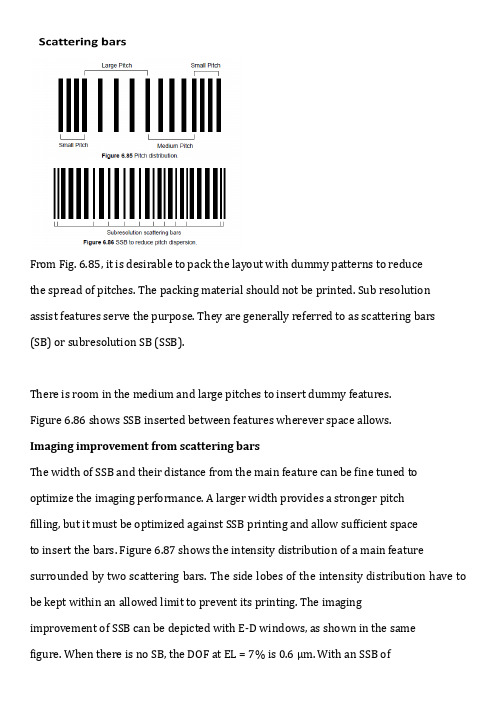
From Fig. 6.85, it is desirable to pack the layout with dummy patterns to reducethe spread of pitches. The packing material should not be printed. Sub resolution assist features serve the purpose. They are generally referred to as scattering bars (SB) or subresolution SB (SSB).There is room in the medium and large pitches to insert dummy features.Figure 6.86 shows SSB inserted between features wherever space allows.Imaging improvement from scattering barsThe width of SSB and their distance from the main feature can be fine tuned to optimize the imaging performance. A larger width provides a stronger pitchfilling, but it must be optimized against SSB printing and allow sufficient spaceto insert the bars. Figure 6.87 shows the intensity distribution of a main feature surrounded by two scattering bars. The side lobes of the intensity distribution have to be kept within an allowed limit to prevent its printing. The imagingimprovement of SSB can be depicted with E-D windows, as shown in the samef igure. When there is no SB, the DOF at EL = 7% is 0.6 μm. With an SSB oftypical width and spacing, the DOF is extended to 0.9 μm. Further customizingof w and S brings the DOF to 1.26 μm.6.3.3.2.1 Restricted pitchThe OAI angle is usually set near the minimum pitch to gain DOF there. TheDOF gradually decreases as pitch increases to an unacceptable level. As soon as space between features allows, SSBs are inserted. Normally, there is an ideal distance from the SSB to the edge of the feature that the SSB is intended to enhance. This is an edge SB (ESB). However, the distance is quite large, andDOF already drops beyond acceptability with a much smaller pitch. Central scattering bars (CSB) are placed at the center of two tight features, regardless of whether the position is optimal, as long as it does not create an unresolvable pitch or become part of the printed image. There may still be a small range of pitches whose DOF is so small that CSB cannot be used. This is the range of restrictedpitch that should be avoided in the circuit design. Figure 6.88 showsthe DOF of a range of pitches from AttPSM using four different QRI settings. The zones for CSB and ESB are marked. The desired 0.4-μm DOF line is drawn. The DOF falls below 0.4 μm in the pitch range between 0.4 and 0.48 μm. This is the range of the restricted pitch with AttPSM 0.55Q0.87, and SSB at a 248-nm wavelength, NA = 0.7, and EL = 8%. The other quadrupole settings are better. Note that DOF is less sensitive to changes in σmin and that the only benefit of a larger σmax is larger DOF at very small pitches.6.3.3.2.2 2D featuresAdding SSB to 2D features is neither as straightforward nor as effective as for1D features. Figure 6.89 shows the design of two polygates with an enlarged portion for contact holes. The original design is perturbed at the edges correctedfor optical proximity effects, which were covered in Sec. 6.1.1. Scattering bars are placed near the pattern edges, but cannot wrap around the features without breaking to prevent ghost images at SSB corners.Mask-making concernsThe broken SSBs pose the risk of the resist falling off during mask making. Short SSBs are vulnerable to fall offs. When the SB is too narrow, resist fall off also happens. Therefore, the width of the SSB must be carefully optimized. A large width prints through, while a small width promotes fall off of the SSB resist during mask making.The small size of the SSB also poses a problem for mask inspection. Scattering bars should not be mistaken as defects by the mask inspection tool. The size of a printable defect usually falls in a similar dimension as that of SSBs. Therefore, the short scattering bars shown in Fig. 6.89 can be mistaken as defects.6.3.3.2.4 Full-size scattering barBy definition, the full-size scattering bar (FSB) has dimensions similar to the main features. Therefore, it is printable and must be removed with an additionaltrim mask. Is it worth the extra cost? Figure 6.90(a) is identical to Fig. 6.88, which illustrates QRI and SSB. Figure 6.90(b) displays a similar DOF versus pitch plot with identical imaging conditions, except that FSBs are used instead of SSBs. In the “no-SB zone” there is no change, which is expected. In the zone where SB can be inserted, FSB clearly out performs SSB. However, it does not help the first group of restricted pitches. Figures 6.90(c) and 6.90(d) show the ED trees for pitches of 260, 450, and 700 nm; the common E-D tree; and the corresponding E-D windows for SSB and FSB, respectively. The feature size is 113 nm, CD tol = ±9 nm, λ = 248 nm, NA = 0.7, and EL = 8%. The E-D trees and corresponding windows are identical at pitches 260 and 450 nm, since no SBs are used. The E-D window for FSBs at P = 700 nm is larger than that for SSBs. The resultant common DOF is also larger for FSBs—480 against 390 nm. Whether it is worth the extra cost to use FSBs depends on whether the DOF required to support mask flatness, mask topography, lens field curvature, focusing tolerance, wafer leveling, wafer flatness, resist thickness, wafer topography, etc., can be met with the 390-nm DOF.Hollow subresolution scattering bars and subresolution assist PSM Hollow SSB (HSSB) assisting opening features, such as holes and line openings, look very similar to the subresolution-assisted PSM. Figure 6.91 shows these two types of features. The only difference between them is phase shifting in the caseof SA PSM. They share the same space limitation; in other words, there must be sufficient space for the assist feature. SA PSM helps isolated features more than HSSB. For spaces suitable for CSB, SA PSM is more vulnerable to printing through. The combination of OAI with SSB is well studied. Combining OAI with SA PSM requires more studies.。
Electronic Raman scattering in quantum dots revisited
a r X i v :c o n d -m a t /0505658v 1 [c o n d -m a t .m e s -h a l l ] 26 M a y 2005Electronic Raman scattering in quantum dots revisitedAlain Delgado a ,Augusto Gonzalez b ,and D.J.Lockwood c∗aCentro de Aplicaciones Tecnologicas y Desarrollo Nuclear,Calle 30No 502,Miramar,Ciudad Habana, C.P.11300,CubabInstituto de Cibernetica,Matematica y Fisica,Calle E 309,Vedado,Ciudad Habana,Cuba cInstitute for Microstructural Sciences,National Research Council,Ottawa,Canada K1A 0R6We present theoretical results concerning inelastic light (Raman)scattering from semiconductor quantum dots.The characteristics of each dot state (whether it is a collective or single-particle excitation,its multipolarity,and its spin)are determined independently of the Raman spectrum,in such a way that common beliefs used for level assignments in experimental spectra can be tested.We explore the usefulness of below band gap excitation and an external magnetic field to identify charge and spin excited states of a collective or single-particle nature.PACS numbers:78.30.Fs,78.67.Hc,78.20.Ls,78.66.FdKeywords:A.Nanostructures;A.Semiconductors;D.Optical properties;E.Inelastic light scatteringI.INTRODUCTIONRaman scattering in semiconductor structures was de-vised more than twenty years ago by Burstein et.al.as a powerful tool for the identification of electronic excitations 1.To the best of our knowledge,experiments on Raman scattering in quantum dots were performed mainly before 1998.2,3,4The lack of theoretical calcula-tions for the relatively large dots used in the experiments (dozens of electrons per dot)made the experimental re-sults less conclusive.A second handicap of the experiments reported in Refs.[2,3,4]is related to the fact that they explored the con-ceptually difficult resonant regime,where the incident photon energy is in resonance with an electronic state in the conduction band.In contrast,the existing (qualita-tive)theory of Raman scattering is expected to be valid only well away from resonance 5.It is usually called the offresonance approximation (ORA),and is well known for missing out the single-particle peaks in the Raman spectrum 6,which are particularly important in the reso-nant regime.In Ref.[3],laser excitation energies 40meV above band gap were used to identify collective states.The physics of Raman scattering under these conditions is expected to be still more complex because of the sud-den increase of level widths with the opening up of the channel for spontaneous emission of longitudinal optical (LO)phonons 7.The positions of collective peaks were computed by means of the ORA 8,which constitutes a nice example of how one can get reasonable results with a theory that does not work in this regime.In the present paper,we review a set of theoretical results on Raman scattering in relatively large quantum dots 9,10,11,12,which were motivated by the experiments described in Refs.[2,3,4].We explore the below band gap excitation regime to study how the ORA is reached.In addition,it isshownFIG.1:Geometry of the Raman experiment:(a)polarized,and(b)depolarized geometry.B.The theorist point of viewThe theoretical representation of a Raman processemerges from the second-order perturbative result for thetransition amplitude14,A fi:A fi∼ int f|H+e−r|int int|H−e−r|iFIG.3:The calculation scheme used in the paper. photon energy loss.In our calculations,we replace thedelta function by a Lorentzian:δ(x)≈Γf/πfunctions.To save time in the calculation of many-electron wave-functions,we computed the matrix elements of Coulomb interactions, α,β|1/r|γδ ,whereα,β,γ,δare arbitrary one-particle states,and stored them in a computerfile. This calculation takes around7days in a personal com-puter.The matrix elements are loaded into the com-puter at the beginning of a calculation,allowing us to solve the nonlinear integro-differential Hartree-Fock(HF) equations for42electrons in a few minutes,or to compute all of the intermediate states entering a Raman process (around10000)in a few days.The HF equations for holes include the electrostaticfield created by the back-ground electrons in the dot,and take account of valence band mixing effects,as described by the Kohn-Luttinger Hamiltonian16.Up to6quantum-well sub-bands are con-sidered in the HF equations for holes.Thefinal states of the Raman process are excited states of the N-electron system.The intermediate states,on the other hand,are states with N+1electrons and one hole.Both kinds of states are computed by means of random-phase-approximation(RPA)like ansatzs for the wavefunctions17,as illustrated in Fig.3.It was already mentioned elsewhere10that,in our opinion,the main lim-itation of using these functions in the present context is not related to the well-known lack of correlation effects in the RPA,but to the incomplete description of the density of energy levels in intermediate andfinal states.Final states are labelled by the quantum numbers∆L and∆S z,which refer to changes(with respect to the ground state)in the total angular momentum and total spin projections along the z axis.Borrowing a terminol-ogy from Nuclear Physics,we speak about monopole exci-tations when∆L=0,dipole excitations when∆L=±1, and quadrupole excitations when∆L=±2.States are further classified by the degree of collectivity,computed with the help of energy-weighted sum rules17.For charge monopole excitations,for example,we have:f∆E f|D0fi|2=2 2A ORAfi∼ α,α′ α|e i( q i− q f)· r|α′ 23( εi× εf)· f ˆz(e†α↑eα′↑−e†α↓eα′↓)+(ˆx+iˆy)e†α↑eα′↓+(ˆx−iˆy)e†α↓eα′↑ i .(6)A few important conclusions may be derived from Eq.(6).First,we notice that only collectivefinal states havea nonvanishing amplitude in this approximation.The SPEs play no role in the Raman process.Indeed,by expanding the exponential in Eq.(6),one can obtainan alternative expression for A ORAfiin terms of multipole operators15.Onlyfinal states having nonzero matrix el-ements of multipole operators will contribute to A ORAfi.6 A second important conclusion is related to the spinselection rule for Raman scattering.Notice that,in Eq.(6),multipole operators that do not alter the spin quan-tum numbers of the initial state are multiplied by thefactor εi· εf.This means that peaks corresponding tocharge operators will appear in the polarized geometry.On the other hand,multipole operators that modify thespin are multiplied by the factor εi× εf and,consequently,Raman peaks corresponding to spin excitations are ex-pected to be seen in the depolarized geometry.III.RESULTSIn the next two subsections,we present results for Ra-man intensities in quantum dots for laser excitation en-ergies below and above band gap.In the former case,no experimental measurements have been performed sofar.We expect weak Raman signals in this regime,butthere are also many advantages such as,for example,theabsence of a luminescence background,a smooth depen-dence of peak intensities on the excitation energy,etc10.On the other hand,in the above band gap excitationregime,our calculations are performed for an excitation window ranging from E gap to E gap+30meV,where E gap is the effective quantum dot band gap.This is sometimes called the extreme resonance region.A.Raman spectra with below band gap excitation The salient features of the Raman spectra in this ex-citation regime are summarized below.1.Dominance of monopole peaksThere are two reasons for thefinal state monopole ex-citations to be the dominant peaks in the Raman spec-trum.First,Raman scattering proceeds via the(virtual) exchange of two photons.Selection rules dictate that the variation of the angular momentum(with respect to the initial state)should be preferably∆L=0,±2,etc.Sec-ond,the band-orbital factor in the matrix elements of H e−r(see Fig.3)provides roughly a factor(qr)l every time a pair is created or annihilated with a pair angular momentum l.As quantum dot dimensions are typically r∼100nm,2,3and the laser wavelength isλ∼700nm, pairs with l=0dominate the process.On the other hand,final state spin excitations in which there is a spinflip with respect to the initial state are de-pressed,as discussed elsewhere10.The Raman amplitude turns out to be proportional to the minority component of the Kohn-Luttinger hole wavefunction.This means that monopole spin excitations in which∆S z=0should be the dominant peaks in the depolarized geometry. We show in Fig.4some spectra in different angular momentum and spin channels for the purpose of com-with excitation energies17.8and18.4meV,respectively. parison.The laser energy is5meV below the band gap, and the incident(and backscattered)angle is equal to 20◦.Charge monopolar,charge quadrupolar,and spin monopolar peaks(with no spinflips)exhibit comparable magnitudes.Dipolar(not shown)or spin-flip excitations lead to Raman peak intensities one or two orders of mag-nitude lower than charge monopolar peaks.2.Smooth dependence of peak intensities on the excitationenergyThe intensities of individual Raman peaks show a smooth dependence on hνi when the latter is below the band gap.This is simply understood from the Eq.(1)for the transition amplitude.From the experimental point of view,it is a nice feature.The identification of individual peaks could not be easier.According to the ORA,as hνi moves away from the band gap,the collective states should start dominat-ing the Raman spectrum.In this way,we can identify the collective and single-particle excitations(mainly the monopolar and quadrupolar ones)by varying hνi.We show in Fig.5the amplitude squared,|A fi|2,computed in the polarized geometry,for three charge monopolarfi-nal states.One of them is the CDE,and the other two are SPEs with excitation energies17.8and18.4meV, respectively.The CDE already becomes the dominant peak when hνi is around3meV below the band gap.73.Correlation between the SPE Raman peaks and thedensity offinal state energy levelsIt is natural to expect Raman peaks to be located there where there is an agglomeration offinal states2.In this paragraph,we take a step further and compare the po-larized Raman spectrum with the density offinal state SPEs(C),and the depolarized spectrum with the density of SPEs(S).This is an attempt to test the spin selection rules,derived from the ORA for the collective excitations, in the SPEs.The comparison is given in Fig.6,where we show results in the monopolar channel.Unexpectedly,the cor-relation is high,particularly in the depolarized geometry. It is instructive to comment on a commonly held belief that the SPEs appear in both polarized and depolarized spectra.Of course,it is true.But it would be better to say that the SPEs(C)appear mainly in the polarized geometry,and the SPEs(S)mainly in the depolarized ge-ometry.This statement is valid at zero magneticfield.4.Breakdown of the polarization selection rules in amagneticfieldIn a magneticfield,the selection rules deduced from the ORA for the collective states are no longer valid at excitation energies close to the band gap.The reason is the magneticfield dependence of energies and wave-functions of intermediate states entering the summation of Eq.(1).The situation is depicted in Fig.7,where monopolar Raman spectra at B=0and1T are drawn. The excitation energy is hνi=E gap−2.5meV.Let us define the polarization ratio of a sin-glefinal state,|f ,as the ratio of|A fi|2in unfavorable and favorable geometries,i.e.,r= |A fi(unfavorable)|2/|A fi(favorable)|2.By favorable we mean the polarized geometry for a charge excitation,and the depolarized geometry for a spin excitation.The polarization ratios for the collective states at B=0are3×10−4for the CDE,and2×10−7for the SDE.That is,an almost perfect fulfillment of the ORA selection rules in spite of the fact that hνi is only2.5meV below band gap.At B=1T,however,these numbers change to0.03and0.17,respectively.The fulfillment of the selection rules for the SPEs is not so evident in Fig.7,because these states,with excitation energies between16and19meV,are not as easily dis-tinguishable as the collective ones.From the data used to draw thisfigure,we can compute r for each SPE.The average polarization ratios at B=0are3×10−3for the SPEs(C),and2×10−4for the SPEs(S).At B=1T, these numbers become0.26and1.1,respectively.That is,the intensities in both geometries become comparable.85.Jump rule at the band gapNear the band gap,the intensities of Raman peaks fol-low an interesting behavior.Let us focus on the collec-tive excitations and compare the intensities of the CDE and SDE peaks as a function of hνi.The results for the monopolar spectra at B=4.5T are shown in Fig.8. We observe a smooth increase of peak intensity in the favorable geometry as hνi approaches the band gap.In the unfavorable geometry,however,the intensity remains practically constant up to the moment when hνi reaches the band gap,where there is a sudden variation.We call this phenomenon the“jump rule”.SPEs also largely follow this rule.B.Raman spectra under resonant excitation We return now to the B=0case,and increase the laser energy to values above the band gap.As mentioned above,we restrict hνi to the interval(E gap,E gap+30 meV)in order to avoid considering phonon effects. Many of the properties discussed in the preceding sec-tion are still valid in the present context.For example, the monopolar and quadrupolar peaks are the most im-portant peaks in the Raman spectrum,and the density offinal state energy levels is correlated with the positions of the principal Raman lines.1.Dominance of SPEsRaman peaks related to SPEs experience a noticeable increase of intensity under resonant excitation.Qualita-tively speaking,one can say that Raman scattering pro-ceeds through a single intermediate state(the one exactly at resonance),which(virtually)decays indiscriminately to the collectivefinal state or to the SPEs.As there is a large number of SPEs,and they are packed in groups, the intensities of the corresponding peaks can be high. This statement is illustrated in Fig.9,where three spectra corresponding to hνi=E gap+5meV,E gap+10 meV,and E gap+15meV,respectively,are shown.In addition,we observe a non-monotonous dependence of peak intensities on hνi.This is a consequence of the fact that,when hνi is varied,a different intermediate state comes into resonance.2.Correlation between the Raman intensities of individual states and the density of intermediate state energy levels Here,we show how by monitoring the intensities of in-dividual peaks as a function of hνi one can obtain infor-mation about the density of energy levels in intermediate states,at least at low excitation energies above the band gap.9In Fig.10,we follow the samefinal states used in Fig. 5,and compare the corresponding|A fi|2for hνi in the interval(E gap,E gap+30meV)with the density of energy levels.Thefirst peak of|A fi|2near5meV above the band gap signals the beginning of a group of energy levels.A second structure is seen near10meV above the band gap,where there is also a threshold.At higher excita-tion energies there is still some correlation between peaks in|A fi|2and peaks in the density of intermediate state energy levels.3.Absence of interference effectsWe now evaluate the contribution of the different in-termediate states entering the summation of Eq.(1)in resonant Raman scattering.The postulate is that the qualitative picture sketched in Sec.III B1is correct: only those intermediate states whose energies are very close to hνi contribute to the Raman amplitude.To ver-ify this,we performed different calculations of A fi,re-stricting the sum over intermediate states to the window (hνi−δE,hνi+δE).There is qualitatively no change in the spectrum whenδE is reduced from10down to2 meV.We compare in Fig.11the magnitude|A fi|2for the spin monopolar peak with∆E f=18meV with the in-dividual contributions of each intermediate state to the energy∆E f=18meV and the contribution of each individual intermediate state to the sum.sum.No strong cancellation effects nor strong coopera-tion effects are apparent.That is,interference effects inA fi are weak under resonant excitation.4.Selection rules in a magneticfieldThe polarization selection rules that follow from the ORA may be tested for excitation energies above the band gap.Surprisingly,they shown to be very well obeyed at zero magneticfield,and break down in a mag-neticfield.The polarization ratio exhibits a strong de-pendence on hνi and on the appliedfield.In quality of example,let us consider the monopole SDE.At zerofield, r is practically zero(10−7when hνi=E gap+5meV). But at B=1T,r varies from1.1at the band gap to0.1 for hνi=E gap+2.5meV.IV.CONCLUSIONSThese theoretical calculations of the Raman spectrum of a many-electron quantum dot in zero and non zero ap-plied magneticfield have revealed intriguing new features and a great sensitivity to the excitation energy.For excitation energies below the band gap,we found Raman spectra dominated by the collective excitations already when hνi=E gap−5meV.The peak intensities depend smoothly on the excitation energy.In zerofield, the simple-minded polarization selection rules–CDE po-larized/SDE depolarized–are very well obeyed even by the SPEs.This means that one can obtain information10about the density offinal state SPEs from the Raman spectra.In an applied magneticfield,these basic selec-tion rules break down,particularly when hνi is increased up to the band gap,where the Raman intensities of the collective excitations in their“forbidden”geometries sud-denly increase to appreciable values.This we termed the Raman intensity“jump rule”,and may help to determine the charge or spin character of a single excitation.A quite different situation is encountered for excitation at energies above the band gap.The Raman peak in-tensitiesfluctuate considerably as the excitation energy sweeps through resonance with intermediate states.In this regime,the SPEs dominate the Raman spectrum, the Raman intensities of individual peaks correlate well with the density of intermediate state energy levels,and there is an absence of interference effects.It would be interesting now to explore experimentally these new features of the electronic Raman spectrum of many-electron quantum dots.AcknowledgmentsPart of this work was performed at the Institute for Mi-crostructural Sciences(IMS),National Research Council, Ottawa.A.D.acknowledges the hospitality and support of IMS.1E.Burstein,A.Pinczuk,and S.Buchner,in B.L.H.Wilson (ed.),The Physics of Semiconductors,Institute of Physics, Bristol,1979.2D.J.Lockwood,P.Hawrylak,P.D.Wang,C.M.Sotomayor Torres,A.Pinczuk,and B.S.Dennis,Phys.Rev.Lett.77 (1996)354.3C.Schuller,K.Keller,G.Biese,E.Ulrichs,L.Rolf,C. Steinebach,D.Heitmann,and K.Eberl,Phys.Rev.Lett. 80(1998)2673.4C.M.Sotomayor-Torres,D.J.Lockwood,and P.D.Wang, J.Electr.Materials29(2000)576.5M.Cardona(ed.),Light scattering in solids,2nd edition, Springer-Verlag,New-York,1982.6Daw-Wei Wang and S.Das Sarma,Phys.Rev.B65(2002) 125322.7H.Htoon,D.Kulik,O.Baklenov,A.L.Holmes,Jr.,T.Tak-agahara,and C.K.Shih,Phys.Rev.B63(2001)241303. 8M.Barranco,L.Colletti,A.Emperador,E.Lipparini,M. Pi,and Ll.Serra,Phys.Rev.B61(2000)8289.9A.Delgado and A.Gonzalez,J.Phys.:Condens.Matter15(2003)4259.10A.Delgado,A.Gonzalez,and D.J.Lockwood,Phys.Rev.B69(2004)155314.11A.Gonzalez and A.Delgado, /cond-mat/0408510,to appear in Physica E.12A.Delgado,A.Gonzalez,and D.J.Lockwood,to be sub-mitted.13T.Brocke,M.-T.Bootsmann,M.Tews,B.Wunsch,D.Pfannkuche,Ch.Heyn,W.Hansen,D.Heitmann,and C.Schuller,Phys.Rev.Lett.91(2003)257401.14R.Loudon,Adv.Phys.13(1964)423.15A.Delgado,A.Gonzalez and E.Menendez-Proupin,Phys.Rev.B65(2002)155306.16G.Bastard,Wave mechanics applied to semiconductor het-erostructures,Les editions de physique,Les Ulis Cedex, 1998.17P.Ring and P.Schuck,The Nuclear Many-Body Problem, Springer-Verlag,New-York,1980.。
BIRTH OF THE UNIVERSE AS QUANTUM SCATTERING IN STRING COSMOLOGY
Abstract
In a Wheeler-De Witt approach to quantum string cosmology, the present state of the Universe arises from the scattering and reflection of the wave function representing the initial string vacuum in superspace. This scenario is described and compared with the more conventional quantum cosmology picture, in which the birth of the Universe is represented as a process of tunnelling “from nothing” in superspace.
Awarded the “Third Prize” in the 1996 Awards for Essays on Gravitation (Gravity Research Foundation, Wellesley Hills, Ma)
—————————– To appear in Gen. Rel. Grav.
The general solution of the classical equations of motion is well known [7], [8] and contains two distinct branches, √ a(t) = a0 tanh | Λt/2|
√ ±1/ 3
,
√ φ = φ0 − ln sinh | Λt|,
纹理物体缺陷的视觉检测算法研究--优秀毕业论文

摘 要
在竞争激烈的工业自动化生产过程中,机器视觉对产品质量的把关起着举足 轻重的作用,机器视觉在缺陷检测技术方面的应用也逐渐普遍起来。与常规的检 测技术相比,自动化的视觉检测系统更加经济、快捷、高效与 安全。纹理物体在 工业生产中广泛存在,像用于半导体装配和封装底板和发光二极管,现代 化电子 系统中的印制电路板,以及纺织行业中的布匹和织物等都可认为是含有纹理特征 的物体。本论文主要致力于纹理物体的缺陷检测技术研究,为纹理物体的自动化 检测提供高效而可靠的检测算法。 纹理是描述图像内容的重要特征,纹理分析也已经被成功的应用与纹理分割 和纹理分类当中。本研究提出了一种基于纹理分析技术和参考比较方式的缺陷检 测算法。这种算法能容忍物体变形引起的图像配准误差,对纹理的影响也具有鲁 棒性。本算法旨在为检测出的缺陷区域提供丰富而重要的物理意义,如缺陷区域 的大小、形状、亮度对比度及空间分布等。同时,在参考图像可行的情况下,本 算法可用于同质纹理物体和非同质纹理物体的检测,对非纹理物体 的检测也可取 得不错的效果。 在整个检测过程中,我们采用了可调控金字塔的纹理分析和重构技术。与传 统的小波纹理分析技术不同,我们在小波域中加入处理物体变形和纹理影响的容 忍度控制算法,来实现容忍物体变形和对纹理影响鲁棒的目的。最后可调控金字 塔的重构保证了缺陷区域物理意义恢复的准确性。实验阶段,我们检测了一系列 具有实际应用价值的图像。实验结果表明 本文提出的纹理物体缺陷检测算法具有 高效性和易于实现性。 关键字: 缺陷检测;纹理;物体变形;可调控金字塔;重构
Keywords: defect detection, texture, object distortion, steerable pyramid, reconstruction
II
Tracing the evolution of massive galaxies up to z sim 3
On the Compton Scattering in String Theory
Oห้องสมุดไป่ตู้ the Compton Scattering in String Theory
Andrea Pasquinucci
1
1,2
and Michela Petrini
1
Dipartimento di Fisica, Universit` a di Milano and INFN, Sezione di Milano via Celoria 16, 20133 Milan, Italy
2
Theory Division, CERN, 1211 Geneva 23, Switzerland
Abstract: We explicitly compute the Compton amplitude for the scattering of a photon and a (massless) “electron/positron” at tree level and one loop, in a four-dimensional fermionic heterotic string model. We comment on the relationship between the amplitudes we compute in string theory and the corresponding ones in field theory.
CERN-TH/97-212 August, 1997
1
Introduction
The computation of scattering amplitudes of string states through the Polyakov formula is one of the most powerful tools we have to study the properties of firstquantized (perturbative) string theories. Computations of tree-level (i.e. genus-zero) scattering amplitudes in closed string theories often appeared in the literature, mostly in the case where the external states are space-time bosonic particles. One-loop, i.e. genus-one, amplitudes have been computed in the case where the external states are space-time bosons. These computations led to many interesting results, in both string theory and field theory. Indeed one can compare directly the scattering amplitudes for the “same” external states in field theory and string theory, or one can take the field-theory limit of a string amplitude and compare it with the field theoretical one. Obviously the two expressions obtained in this way must be identical, but the way in which string theory reproduces the field theoretical amplitudes can lead to the discovery of new features of field theory (see for instance refs. [1, 2, 3]). Very few one-loop amplitudes having space-time fermions as external states have appeared in the literature (see for example ref. [4]), mostly because of some technical issues appearing in the explicit computations of these amplitudes, as discussed for example in ref. [5]. In this paper we present one of the simplest four-point one-loop scattering amplitude, which involves external space-time fermions, that is the Compton scattering of an “electron/positron” and a photon. Here we call “electron” (or “positron”) a massless space-time fermion charged under a U (1) component of the total gauge group. This state does not correspond directly to what we would usually call a, let us say, electron, since it is massless, charged under other components of the total gauge group, and also carries some (stringy) family labels. One can easily extend the results we present in this letter to the case of the scattering of a massless “quark” on a gluon, since this requires only some simple modifications of the left-moving part of our equations. In doing these computations, we have chosen a specific “simple” four-dimensional heterotic string model. One of the particular properties of this model is that its space-time spectrum depends on a set of parameters and, as described in ref. [5], only for some values of these parameters is supersymmetric. Of course the string scattering amplitudes depend on the particular spectrum and on the details of the
D-Brane Scattering of N=2 Strings
a rXiv:h ep-th/01869v11A ug21D-Brane Scattering of N =2Strings Klaus J¨u nemann a and Bernd Spendig b a E-mail:K.Junemann@ b Institut f¨u r Theoretische Physik,Universit¨a t Hannover Appelstraße 2,30167Hannover,Germany E-mail:spendig@itp.uni-hannover.de Abstract The amplitudes for emission and scattering of N =2strings offD-branes are calculated.We consider in detail the amplitudes cc and occ for the different types of D-branes.For some D-branes we find massive poles in the scattering spectrum that are absent in the ordinary N =2spectrum.1IntroductionIt has become obvious in the last couple of years that D-branes are of utmost importance for our understanding of N=1string theory.In his pathbreaking paper[1],Polchinski showed that p-dimensional extended objects–the D-p-branes–are the the long sought carriers of the Ramond-Ramond charges in N=1string theory.In the context of scattering amplitude calculations the most important property of D-branes is that their quantumfluctuations are described by open strings moving on the brane and therefore are under good control at weak coupling(for reviews on D-branes see e.g.[2,3]and literature cited within).This allows to calculate amplitudes for emission and scattering of closed fundamental strings from D-branes by”pre-revolutionary”methods that have been invented more than a decade ago and are well understood[4].For the N=1string these computations have been performed e.g.in refs.[5,6,7,8,9]and considerably contributed to the understanding of D-brane physics.It is the purpose of this note to perform a similar analysis for N=2strings.That this analysis has not been undertaken so far for the N=2stringfinds its reason in the lack of Ramond-Ramondfields in the string spectrum.The N=2superconformal algebra with c=6serves as constraint algebra and is powerful enough to remove all string excitations from the spectrum leaving the center of mass motion(which is not tachyonic but massless in this case)as the only physical degree of freedom[10].This has immediate consequences for possible interactions.All n-point functions vanish[11],the only non-vanishing tree-level amplitude is the3-point function. The correspondingfield theory is self-dual gravity for closed strings and self-dual Yang-Mills theory for the open string sector.The critical dimension of the N=2string is four but with“unphysical”signature(2,2),making it possible to identify the four real with two complex dimensions. Although lacking the necessary Ramond-Ramondfields,it is still possible to formally define D-branes in N=2string theory by imposing Dirichlet boundary conditions in certain target space directions.The obvious question is then whether the closed N=2strings feel the presence of the branes.This note gives an answer to this question by performing a scattering analysis similar to the one undertaken in[7]for N=1strings.2ConventionsWe choose theflat target-space metric asηµν=diag(−+−+).It is advantageous to subsume the real(2,2)-vectors into complex(1,1)-vectors with metricηµν=diag(−,+).In detail:X±=(X±0,X±1)=(X0±iX2,X1±iX3).(1) The(2,2)-scalar product written in components readsX1·X2=12 X++1X−−2+X+−1X−+2 ,where X±+=X±0+X±1and X±−=−X±0+X±1.Moreover,we introduce the matrices Jk+·p−=k·p+ik·J·p.(2) (J acts as a self-dual complex structure.It is J02=J13=1,J13=J02=−1,all other elements =0),andDµν=diag(D00,D11,D22,D33).(3) This matrix D is related to theflat target space metricηby a change of sign in the directions transverse to the D-brane.Example:Let x2be the only direction transverse to the D-brane.Then D=diag(−+++).Emission and scattering offD-branes is conveniently calculated by evaluating correlators between vertex operators on the upper half plane.Open strings are represented by holomorphic vertex operators restricted to live on the real axis whereas closed string vertex operators factorize into holomorphic and antiholomorphic parts,V cl(z,¯z,p)=:V(z,p/2)::V(¯z,p/2):.(4) Here z lies inside the upper half plane.The sum of each picture number has to add up to−2inside a non-vanishing scalar product.We will use vertex operators in the(−1,−1),(−1,0)and(0,−1) picture[12]:V(−1,−1)(k,z)=e−ϕ−−ϕ+e ik·X(z),V(−1,0)(k,z)=k+·ψ−e−ϕ−e ik·X(z),V(0,−1)(k,z)=k−·ψ+e−ϕ+e ik·X(z).(5) 3The general calculationsThe separate propagators for holomorphic and antiholomorhicfields are standard.However,due to the presence of a world sheet boundary,there are also non-vanishing correlation functions between holomorphic and antiholomorphicfields[7,13,14]:Xµ(z)Xν(¯w) =−Dµνln(z−¯w),ψµ(z)ψν(¯w) =−Dµνk−·(G+·p)+,z−¯wk+·ψ−(z)p+·ψ−(¯w)∼−1k+·(G−·p)−,z−¯wk−·ψ+(z)p+·ψ−(¯w)∼−1with the definition G±=D±J·D·J.The D-brane respects the complex structure in target space if G+=0,i.e.D=−J·D·J.The new feature here(as compared e.g.to the mixed amplitudes)is that for Dirichlet boundary conditions in general one gets poles in the operator product expansion between holomorphic and antiholomorphicfields both having a+or−index.3.1A ccIt was shown in ref.[7]that the scattering amplitude of two N=1closed strings offa D-brane can be obtained from the N=1open string4-point function by simply interchanging certain momenta. Thus the amplitude takes the form of an Euler-Beta-function of the Mandelstam variables that can be expanded as an infinite series of closed string poles in the t-channel or of open string poles in the s-channel and leads to the soft high energy behavior of the amplitude[5].This result is intuitively clear since the interaction of closed strings with a D-brane is mediated by exchange of closed strings travelling between the passing closed string and the D-brane,or–via world sheet duality–by open strings moving along the brane.This argument should also be true in N=2string theory.But it is difficult to imagine what a dual amplitude could look like in a theory with only a single degree of freedom.We therefore expect the scattering amplitude of a closed N=2string offa D-brane to vanish1.The scattering amplitude of two closed strings offa D-brane for the N=2string is given by the integral of the correlation function of two closed string vertex operators with the correct quantum numbers over the upper half-plane H+:A cc(p1,p2)∼ H+d2z d2w V(−1,0)(z,p1/2)V(−1,0)(¯z,p1/2)V(0,−1)(w,p1/2)V(0,−1)(¯w,p1/2) .(8) Momentum conservation holds only in directions parallel to the brane:p12+p22=0,p21=p22=0,(9)where p1and p2denote the momenta of the incoming and outgoing strings,respectively.In analogy to4-particle scattering the amplitude can be parametrized by the following Mandelstam variables:s=(p12)2,t=(p12)2,u=(p12)2.(10)Obviously s is the momentum transfer along the brane and t is the amount of momentum absorbed by the brane.As usual s+t+u=0.SL(2,R)invariance of the correlation functions on the upper half plane allows us tofix three of the four variables of the vertex operators.For A cc we choose z=iy(y∈R+)and w=i.The correct integration measure is 10dy(1−y2).The resulting expression can be transformed into well known integral-representations of Euler-Beta-functions using the“miracle”-substitutiony=1−x1/2Γ(s+t)+BΓ(s)Γ(t)Γ(s+t+1)(12)withA=p+1·(G+·p1)−p−2·(G+·p2)+,B=4(p+1·p−2)2,C=(p+1·(G−·p2)−)2.3.2A oocThe amplitude for two open strings on the brane joining into an outgoing closed string isA ooc(k1,k2,p)∼ R,x<y dx dy H+d2z× V(−1,0)(x,k1)V(−1,0)(y,k2)V(0,−1)(z,p/2)V(0,−1)(¯z,p/2)x and y are integrated along the real axis in such a way that x is always left of y.The momenta k i of the open strings have to be parallel to the brane which implies k i=D·k i.Momentum conservation in this case readsk1+k2+p2D·p=0There is only a single kinematical variable s=k1·k2=12p·k1=−1(1+y2)b =√2)Γ(a+1)Γ(2b−a−1)2a+1)Γ(b−12)Γ(a)=√Γ2(1−t).(13)This expression is completely analogous to that of the N=1theory.4Evaluating the general results for each D-brane-typeIn this section the above amplitudes are explicitly analyzed for each type of D-brane.Due to the special signature(2,2)of our space-time we denote the D-branes by p+q,where p and q are the number of spatial and time directions,respectively,in which the D-brane lives.4.1The(2+2)brane4.1.1A ccIn this case the branefills all of space-time and we have ordinary interaction between open and closed strings that has been considered in[15,16].A cc has the interpretation of the lowest order quantum correction to closed string propagation.Momentum conservation holds in all directions for closed string scattering offthe2+2brane.We cannot use our result,though,since byfixing three real parameters before integrating we did not divide out the volume of the whole symmetry group,which is,as we are dealing with a closed string topology SL(2,C)rather than SL(2,R). Naive application of our result(12)would lead to A cc=0,while the real amplitude is known to be constant.4.1.2A oocFor the process of joining of two open strings into a closed string momentum conservation implies that p·k1=p·k2=k1·k2=0.Since s=12(p31)2and u=0.What onefinds from eq.(12)is thatthefirst two terms vanish because the denominator diverges at u=0.The third term reduces toA cc∼−(p+1(G·p2)−)2Γ(s)Γ(1−s)=−4[(p01)2+(p21)2]Γ(s)Γ(1−s).(16) Now usingΓ(s)Γ(1−s)=πsin(πs).(17)4.2.2A oocAgain we demand Dirichlet boundary conditions in the3-direction.G−=diag(0,−2,0,−2).The kinematics read k31=k32=0.We have to distinguish between two casesa)k33=0Here t=0,thus we end up with afinite amplitude:A ooc∼k+13k+2·(G−·k3)−.b)k33=0We getA ooc∼Γ(1−2t)Γ(1−t)∼cos(π·(1/2−t))Γ(1/2−t)Γ(t).This amplitude has a tachyonic pole.4.3The(1+1)brane4.3.1A ccFor this kind of brane the matrix D satisfies the relation D=J·D·J which implies G−=C=0 and G+=2D.The closed string scattering amplitude becomesp+1·(D·p1)−p−2·(D·p2)+Γ(s+t).(18)A cc∼To further analyze the kinematical prefactor one recalls that in2+2dimensions four momentum vectors with 41k i=k2i=0satisfy the relation[11](k+1·k−3)(k+2·k−4)k1·k4+(k+1·k−4)(k+2·k−3)k1·k3=0.(19) It is this equation that is responsible for the vanishing of the4-point function in open and closed N=2string theory.Settingk1=p1,k2=D·p2,k3=D·p1,k4=p2and using the fact that(Dp1)−·(Dp2)+=p+1·p−2for this particular form of D,onefinds that(p+1·(D·p1)−p−2·(D·p2)+)t+(p+1p−2)2s=0.What remains isA cc∼(p+1·p−2)2Γ(s−1)Γ(t)4.4The(0+2)brane4.4.1A ccTwo time dimensions with Dirichlet boundary conditions imply that D=−J·D·J and therefore G+=A=0and G−=2D=2diag(++++).The scattering amplitude isA cc∼[(p+1·p−2)2u+(p1·(Dp2)−)2t]Γ(s)Γ(t)u(s−1) Atu+Bu(s−1)+Ct(s−1) Γ(s)Γ(t)4.6The(0+0)brane/D-instanton4.6.1A ccDirichlet boundary conditions in all directions imply for the scattering process that there is no relation between the momenta of the incoming and outgoing closed strings.Since D=−ηthe Mandelstam variables and kinematical factors becomes=14p1·p2,A=0,B=C=4(p+1·p−2)2.The scattering amplitude in this case isA cc∼(p+1·p−2)2 Γ(t)Γ(s)Γ(t+s+1) ,(25) leading to a simple1y(x+iy)(x2+y2)α((1−x)2+y2)β(α,β∈R).So far we have not been able yet to solve this integral.6ResultsWefind that if the D-brane breaks the complex structure in target space additional correlation functions appear in the calculation which are absent for the usual Neumann boundary conditions. The result for the amplitude A cc is nevertheless an Euler Beta-function multiplied by a kinematical prefactor.A closer look at this kinematical factor shows that the amplitude vanishes only for the 2+2and the0+2brane and has a single simple pole at t=0for the D-instanton which is dueto closed string exchange.The scattering amplitudes of branes that break the complex structure in target space,i.e.the1+2,the1+1and0+1brane all have poles that do not correspond to states in the spectrum of the N=2string.How do we interpret these results?In this paper we have considered the N=2string in its gauge fixed NSR formulation.Massive poles in the scattering spectrum seem to be inconsistent with this type of string.The inconsistency can be traced back to the fact the presence of these branes conflicts with N=2world sheet supersymmetry.This is due to the fact that a fermionψobeying Dirichlet boundary conditions cannot be in the same multiplet as a fermion obeying Neumann boundary conditions.This breaking of N=2world sheet supersymmetry hence seems to leave no space for these type of branes in the gauge-fixed NSR formulation of the N=2string.This result is also consistent with T-duality.Recall that Neumann and Dirichlet boundary con-ditions are interchanged upon performing a T-duality transformation in a toroidally compactified space-time.However,for N=2string propagation only Ricci-flat K¨a hler manifolds with(2,2)sig-nature are allowed.This leaves only the possibility to compactify one or both complex directions. Compactification of one or three real coordinates breaks the complex structure and yields an illegal background.Fortunately the three relevant branes,namely the2+2-and0+2-brane and the D-instanton,form a closed set under the action of T-duality in the allowed backgrounds.Apart from the2+2-brane the other relevant branes are non-dynamical since open strings attached to them have vanishing momentum2.This means that dynamical D-branes do not exist in the NSR formulation of N=2string theory in accordance with the absence of the corresponding differential forms and solutions of the classical equations of motion.We want to mention,though,that our formulation is not the only one that is able to describe the N=2string.As was shown by Berkovitz and Vafa[17]and Siegel[18]there exists as well a more general formulation of the N=2string in terms of the so-called topological N=4string.This formulation admits more degrees of freedom and hence there might be a way how the forbidden branes can be consistently incorporated in N=2 string theory.But so far no attempt in this direction has been made,leaving room for further work and speculations.AcknowledgementsWe would like to thank O.Lechtenfeld for many fruitful discussions.B.S.thanks the Studienstiftung des deutschen Volkes for support.References[1]J.Polchinski,Phys.Rev.Lett.75(1995)4724,hep-th/9510017[2]C.P.Bachas,Proceedings of the31st International Symposium Ahrenshoop in Buckow,hep-th/9806199.[3]J.Polchinski,TASI Lectures on D-branes,hep-th/9611050.[4]D.Friedan,E.Martinec,and S.Shenker,Nucl.Phys.B271(1986)93.[5]I.R.Klebanov,L.Thorlacius,Phys.Lett.B371(1996)51,hep-th/9510200.[6]S.S.Gubser,A.Hashimoto,I.R.Klebanov,J.M.Maldacena,Nucl.Phys.B472(1996)231,hep-th/9601057.[7]M.R.Garousi,R.C.Myers,Nucl.Phys.B475(1996)193,hep-th/9603194.[8]A.Hashimoto,I.R.Klebanov,Phys.Lett.B381(1996)437,hep-th/9604065.[9]A.Hashimoto,I.R.Klebanov,Nucl.Phys.Proc.Suppl.55B(1997)118,hep-th/9611214.[10]H.Ooguri and C.Vafa,Nucl.Phys.B361(1991)469.[11]R.Hippmann,http://www.itp.uni-hannover.de/˜lechtenf/Thesis/hippmann.ps[12]J.Bischoff,S.V.Ketov,and O.Lechtenfeld,Nucl.Phys.B438(1995)37,hep-th/9406101.[13]M.Ademollo,A.D’Adda,R.D’Auria,E.Napolitano,P.Di Vecchia,F.Gliozzi and S.Sciuto,Nucl.Phys.B77(1974)189.[14]M.Frau,I.Pesando,S.Sciuto,A.Lerda,R.Russo,Phys.Lett.B400(1997)52,hep-th/9702037[15]N.Marcus,Nucl.Phys.B387(1992)263.[16]B.Spendig,http://www.itp.uni-hannover.de/˜spendig/works/prolog1.ps[17]N.Berkovitz,C.Vafa,Nucl.Phys.B433(1995)123,hep-th/9407190.[18]W.Siegel,Phys.Rev.Lett.69(1992)1493,hep-th/9204005.10。
外文翻译原文Gamma scattering scanning of concrete block for detection of voids
Gamma scattering scanning of concrete block for detection of voids.Shivaramu 1,Arijit Bose 2and M.Margret 11Radiological Safety Division,Safety Group,IGCAR,Kalpakaam -603102(India)2Chennai Mathematical Institute,Sipcot I.T.Park,Chennai -603103(India)E-mail:shiv@.in,arijitbose@cmi.ac.in Abstract The present paper discusses a Non Destructive Evaluation (NDE)technique involving Compton back-scattering.Two 15cm x 15cm x 15cm cubical concrete blocks were scanned for detection of voids.The setup used a PC controlled gamma scattering scanning system.A 137Cs radioactive source of strength 153.92GBq with lead shielding and a collimated and shielded 50%efficiency coaxial HPGe detector providing high resolution energy dispersive analysis of the scattered spectrum,were mounted on source and detector sub-assemblies respectively.In one of the concrete blocks air cavities were created by insertion of two hollow cylindrical plastic voids each of volume 71.6cm 3.Both the concrete blocks,one normal and another with air cavities were scanned by lateral and depth-wise motion in steps of 2.5cm.The results show that the scattering method is highly sensitive to changes in electronic and physical densities of the volume element (VOXEL)under study.The voids have been detected with a statistical accuracy of better than 0.1%and their positions have been determined with good spatial resolution.A reconstruction algorithm is developed for characterization of the block with voids.This algorithm can be generally applied to such back-scattering experiments in order to determine anomalies in materials.Keywords:Gamma backscattering,Non-Destructive Evaluation,Compton scattering,HPGe detector,Voids,VOXEL,reconstruction algorithm.1Introduction The need for advanced techniques for detection and evaluation of a class of sub-surface defects that require access only to the one side of any material or structure relatively thick to be inspected has drawn attention to X-ray or gamma backscatter as a desirable choice [1-3].There is a great demand for non-destructive testing and evaluation (NDT,NDE)techniques in many diverse fields of activity.A particular area of interest is encountered in detection of defects in concrete structures.Ultrasonic,Radiography and Compton Back Scattering techniques are currently employed to test the components of structures.Transmission provides line-integrated information along the path of radiation from the source to the detector,which masks the position of an anomaly present along the transmission line.Therefore,it is difficult to determine the position of an anomaly directly from transmission measurements.The backscatter technique can image a volume rather than a plane.Point-wise information can be obtained by focusing the field of view of the source anddetector so that they intersect around a point.Since both the source and detector are located on the same side of the object,examination of massive or extended structures become possible.This NDE technique should be developed as it can be applied in:•Detection of corrosion in steel liners that are buried (covered by concrete),detection of voids >20mm diameter in concrete.Detection of flaws before they propagate to the point of causing failure is essential.•Locating flaws in nuclear reactor walls or dam walls.•Detection of landmines.a r X i v :0912.1554v 2 [c o n d -m a t .m t r l -s c i ] 5 J a n 2010Therefore an urgent need exists to develop diversified and effective NDE technologies to detectflaws in structures.The gamma scattering method is a viable tool for inspecting materials since it is strongly depen-dent on the electron density of the scattering medium,and in turn,its mass density.The concept is based on the Compton interaction between the incident photons and the electrons of matter.Gamma or X-rays scattered from a VOXEL are detected by a well-collimated detector placed at an angle which could vary from forward scattering angles to the back-scattering configuration.The scattered signal,therefore,provides an indication of the electron density of the material comprising the inspected volume[4].By scanning a plane of interest of the object,it is possible to obtain the density distribution in this plane.In this process scattered signals are recorded from different depths of the material.Hence,gamma scattering enables the detection of local defects and the discrimination between materials of different density and composition,such as concrete,void and steel.Moreover,in NDT,the nature of the inspected object is usually known and the purpose is to determine any disturbance in the measured signal that can indicate the presence of an anomaly.Two concrete blocks one normal and another with air cavities were scanned completely by voxel method. The inspection volume(voxel)was formed by the intersection of the collimated incident beam cone and the collimatedfield of view of the HPGe detector.The corresponding Compton scattered spectrums of these two blocks were compared and analyzed.As the void intersected the sensitive volume,there was a decrease in the total electron density of the material comprising the voxel,hence it showed a decrease in detector response.The presence of void could be clearly distinguished and located.2Experimental ProcedureThe schematic of the experimental set up is shown in Fig.1.The scanning system consists of source and detector unit and a four axis job positioning system for moving the block.The source and detector units are composed of a positioning stage,a fabricated base and common to both unit is a control panel and a Laptop.The positioning stages of each unit consist of X,Y-axis travel stage,Z-axis vertical travel stage and a rotary stage.The137Cs radioactive source of strength153.92GBq with a lead shielding and the collimated and shielded50%efficiency coaxial HPGe detector,providing high resolution energy dispersive analysis of the scattered spectrum,are mounted separately on the source and detector sub-assemblies of6-axis system respectively.The concrete blocks are mounted on the4-axis job positioning system.The voxel to be analyzed is geometrically established by the intersection of the incident and scattered beams.The size of the voxel is defined by the diameter and length of the collimators employed and on source to object,detector to object distances and can be easily chosen by proper adjustment of X, Y,Z andθpositions of6-axis and4-axis job positioning systems.The source and detector is collimated with solid lead cylindrical collimators of diameter17and3mm respectively,and the size of the resulting voxel is19cm3.The scattered intensity from a voxel in the concrete block is detected and the pulse height spectrum(PHS)is accumulated and displayed using an8K-channel analyzer which is interfaced with a PC for data storage and analysis.The scattering angle is96◦and the incident photon energy emitted by137Cs is661.6keV and the energy of the scattered photon is273.6keV(Compton scattering).Two concrete blocks one normal and another with air cavities,created by inserting two hollow cylindrical plastic voids of diameter39mm and height60mm,are chosen for void detection and quantification.These voids were placed at equal distances from the surface and from the centre of concrete block symmetrically as shown in Fig.1.The horizontal and depth-wise scanning of a plane in the concrete cube was performed by moving the blocks across the source and detector collimators in steps of2.5cm.The photo peak counts of the scattered spectrum for corresponding positions of both the specimens of concrete blocks one normal and another withair cavities were compared and analyzed.3Reconstruction Algorithm and Attenuation CorrectionsThe reconstruction algorithm developed to correct for attenuation of the incident and scattered photons by the material surrounding each scatter site is described.It provides accurate reconstruction of the Compton scattering data through an adequate correction of the absorption phenomena.The path from the source to detector can be broken into three stages.Thefirst stage is the photon’s travel from the source to the scattering point P along the pathα.Neglecting attenuation due to air,from Beer-Bougher law:I1=I0exp−xµ(E)ρρdx(1)Where I1and I0are the transmitted and incidentflux,respectively,µ(E)ρis the mass attenuation coefficientof the material for photons of energy E,ρis the density of the material and x is the length of pathαin block[5].The second stage is scattering towards detector at point P.The scatteredflux I2is determined by;I2=I1dσdΩ(E,θ)S(E,θ,Z)dΩρe(P)∆L(2)WheredσdΩ(E,θ)is the differential scatter cross section as governed by the Klein-Nishina formula(a function of the incident gamma energy E and scatter angleθ),S is the incoherent scattering function(a function of E,θand atomic number of the element Z),dΩis the solid angle subtended by the detector and its collimator,ρe(P)is the electron density at point P and∆L is an element of pathαin the vicinity of point P(the voxel thickness).The electron density at P is the material property we are attempting to measure. It is proportional to the physical densityρaccording to the formula:ρe=ρNZA[6],where N is Avogadro’s number,Z is atomic number and A is atomic weight.The third stage is the transport of scattered photons back through material to detector.The signal is further attenuated,so that:I3=I2exp−x sµs(E s,θ)ρρdx(3)here I3is theflux intensity reaching the detector,µs(E s,θ)ρis the mass attenuation coefficient for scatteredphotons of energy E s,now a function ofθby the virtue of the Compton energy shift at P,and x s is the length of the pathβin the bining the expressions for the three stages,the signal intensity corresponding to point P can be written as,I3=I0exp−xµ(E)ρρdx +x sµs(E s,θ)ρρdxdσdΩ(E,θ)S(E,θ,Z)dΩρe(P)∆L(4)Letk=dσdΩ(E,θ)S(E,θ,Z)dΩNZA∆L(5)The attenuation factor is,AF=exp−[x0{µ(E)ρ}ρdx +x s{µs(E s,θ)ρ}ρdx ](6)In the present case as per Fig.2;AF=exp−[T0{µ(E)ρ}ρdtcosθ1+T{µs(E s)ρ}ρdt scosθ2(7)combining(4),(5)and(6)we get,I3=I0kρ(P)AF(8) Taking the ratio of I3which is experimentally the counts under the photo peak of Compton scattered spectra for normal concrete block(Block1)and another with air cavities(Block2)we get,I3(Block2) I3(Block1)=ρ(P,Block2)AF(P,Block2)ρ(P,Block1)AF(P,Block1)(9)The attenuation factor for normal concrete block can be calculated just by substituting the mass attenuation factor and density of concrete in(7).For calculating the attenuation factor for different VOXEL positions of concrete block with air cavities one requires the geometry and hence the path length traveled by incident and scattered rays in void and concrete.This information is obtained using software graphics.Here the knowledge of the precise location and size of the voids are used.We see that equation(9)is iteration in density.We can either take up iteration approximations to obtain the void locations in case of voids of unknown location and sizes.Other alternatives are:•reduction of VOXEL size which will give a better spatial resolution and contour of the voids•or changing the scattering angle and generating more density distribution pictures of the concrete block under investigation andfinally superimposing the results.4Results and DiscussionThe lateral variation of the difference in Compton photo peak counts of the scattered spectrum between normal and void incorporated concrete block,measured at7.5cm from the bottom,for various depths (D0:-front face to D3:-center each2.5cm apart)are shown in Fig.3and4.The density ratio of the two concrete blocks derived from the equation(9)plotted as a function of lateral distance is shown in Fig.5.As the sensitive volume intersects the void cavity,there is a reduction in the total electron density and hence increase in the difference scattered intensity(Figs.3&4)and decrease in density ratio(Fig.5).At the front face of the blocks(D0)it is known that there is no void coming into the investigation voxel and the same can be inferred from the results shown in Figs.3,4&5which show same scattered intensity and hence density. On the other hand at5cm depth from the front face(D2)the effect of the voids can be seen(Figs.3&4) as a U shaped scattered intensity curve and an inverted U shaped density ratio(Fig.5).The magnitude ofthe difference in scattered intensity(Figs.3&4)and decrease in density(Fig.5)is proportional to the size of the void within the voxel.This gives an idea of the size and location of the void as the voxel size and its orientation in concrete is known for all positions.The voxel size was estimated as85cm3in the present case. The cylindrical voids have been detected in the present study with a statistical accuracy of better than0.1%. It is also possible to locate the position of the voids successfully even without considering the contribution due to the attenuation factor.The effectiveness of this inspection technique can be defined by the spatial resolution and the density contrast achievable.Good resolution requires a small sensitive volume,while high contrast demands large sensitivity to changes in composition.The size of the inspection volume defines the spatial resolution.Reducing the collimator aperture to improve the spatial resolution leads,however, to a decrease in the count rate.This can be compensated for by increasing the source strength and the counting period.A practical compromise is therefore necessary to achieve a reasonable resolution within an appropriate counting period and without exposure to a high dose of radiation.In order to increase the contrast,the contribution to the detector from the material contained within the sensitive volume should be enhanced while that of the surrounding media should be reduced.This can be achieved by reducing the attenuation of the radiation as it travels to and from the sensitive volume,and/or by increasing the probability of scattering within the volume.The attenuation and scattering probability,however,depend on the radiation energy and the angle of scattering.The incident angle,defined in Fig. 2.determines the photon path length and in turn affects the attenuation probability.The source energy and the scattering angle are,however,the two most important design parameters as they directly affect the detector response.Fig.3.The difference Compton photo peak countsFig.4.The2D bar graph of difference Compton photo peak countsFig.5.The density ratio as a function of lateral distance5Referenceswson,L.,¨Backscatter Imaging¨,Materials Evaluation,60(11),1295-1316,20022.Harding G,Inelastic photon scattering:Effects and applications in biomedical science and industryRadiation Phys.Chem.1997,50,91-1113.Hussein E M A Whynot T M,A compton scattering method for inspecting concrete structures Nucl.Instr.Method1989,A283,100-1064.P Zhu,P Duvauchelle,G Peix and D Babot:X-ray Compton backscattering techniques for processtomography:imaging and charecterization of materials;Meas.Sci.Technol.7.5.C.F.Poranski,E.C.Greenawald and Y.S.Ham;X-Ray Backscatter Tomography:NDT Potential andLimitations;Materials Science Forum Vols.210-213(1996)pp.211-218.6.R.Cesareo,F.Balogun,A.Brunetti,C.Cappio Borlino,90o Compton and Rayleigh measurements andimaging;Radiation Physics and Chemistry61(2001)339-342.6Acknowledgements•Dr.N.Mohankumar,Head,Radiological Safety Division,IGCAR,Kalpakkam.•Ramar,IGCAR.•Priyada,IGCAR.。
- 1、下载文档前请自行甄别文档内容的完整性,平台不提供额外的编辑、内容补充、找答案等附加服务。
- 2、"仅部分预览"的文档,不可在线预览部分如存在完整性等问题,可反馈申请退款(可完整预览的文档不适用该条件!)。
- 3、如文档侵犯您的权益,请联系客服反馈,我们会尽快为您处理(人工客服工作时间:9:00-18:30)。
arXiv:hep-th/0610062v3 23 Nov 2006
Department of Electrophysics, National Chiao-Tung University, Hsinchu, Taiwan, R.O.C. Yi Yang‡ Department of Electrophysics, National Chiao-Tung University and Physics Division, National Center for Theoretical Sciences, Hsinchu, Taiwan, R.O.C.
Scatterings of Massive String States from D-brane and Their Linear Relations at High Energies
Chuan-Tsung Chan∗ Department of Physics, , R.O.C. Jen-Chi Lee†
(Dated: February 2, 2008)
Abstract
We study scatterings of bosonic massive closed string states at arbitrary mass levels from Dbrane. We discover that all the scattering amplitudes can be expressed in terms of the generalized hypergeometric function 3 F2 with special arguments, which terminates to a finite sum and, as a result, the whole scattering amplitudes consistently reduce to the usual beta function. For the simple case of D-particle, we explicitly calculate high-energy limits of a series of the above scattering amplitudes for arbitrary mass levels, and derive infinite linear relations among them for each fixed mass level. The ratios of these high-energy scattering amplitudes are found to be consistent with the decoupling of high-energy zero-norm states of our previous works.
simple case of D-particle, we explicitly calculate high-energy limit of a series of the above scattering amplitudes for arbitrary mass levels, and derive infinite linear relations among them for each fixed mass level. Since the calculation of decoupling of high energy ZNS remains the same as the case of scatterings without D-brane, the ratios of these high-energy scattering amplitudes are found to be consistent with the decoupling of high-energy zeronorm states of our previous works. [5, 6, 7, 8, 9, 10, 11, 12]. This paper is organized as follows. In section II, we first calculate closed string tachyon scatters to D-brane. The calculation is then generalized to arbitrary mass levels. By using the Kummer relation of the hypergeometric function 2 F1 , all the scattering amplitudes in the (0 → 1) and (1 → ∞) channels can be reduced to the usual beta function. We then sum up the (0 → 1) and (1 → ∞) channels, and show that all the scattering amplitudes can be expressed in terms of the terminated generalized hypergeometric function 3 F2 with special arguments, and the whole scattering amplitudes consistently reduce to the usual beta function. In section III, for the simple case of D-particle, we explicitly calculate high-energy limit of a series of the above scattering amplitudes for arbitrary mass levels, and derive the linear relations among them. The results are compared to the calculations of decoupling of high energy ZNS. We give a brief conclusion in section IV. Some relevant formulas of the hypergeometric function
∗ † ‡
Electronic address: ctchan@.tw Electronic address: jcclee@.tw Electronic address: yyang@.tw
1
I.
INTRODUCTION
In contrast to the scattering of massless string states, massive higher-spin string scattering amplitudes [1] had not been well studied in the literature since the developement of string theory. Recently high-energy, fixed angle behavior of string scattering amplitudes [2, 3, 4] was intensively reinvestigated for massive string states at arbitrary mass levels [5, 6, 7, 8, 9, 10, 11, 12, 13]. The motivation was to uncover the fundamental hidden stringy spacetime symmetry. An important new ingredient of this approach is the zero-norm states (ZNS) [1, 14, 15, 16] in the old covariant first quantized (OCFQ) string spectrum. One utilizes the decoupling of ZNS to obtain nonlinear relations or on-shell Ward identities among string scattering amplitudes. In the high energy limit, many simplications occur and one can derive linear relations among high-energy scattering amplitudes of different string states at each fixed but arbitrary mass levels. Moreover, these linear relations can be used to fix the ratios among high energy scattering amplitudes of different string states at each fixed mass level algebraically. This explicitly shows that there is only one independent component of high-energy scattering amplitude at each mass level. On the other hand, a saddle-point method was also developed to calculate the general formula of tree-level highenergy scattering amplitudes of four arbitrary string states to verify the ratios calculated above. This general formula expresses all high-energy string scattering amplitudes in terms of that of four tachyon as conjectured by Gross in 1988 [3]. In this paper, we study scatterings of bosonic massive closed string states at arbitrary mass levels from D-brane. The scattering of massless string states from D-brane was well studied in the literature and can be found in [17]. Since the mass of D-brane scales as the inverse of the string coupling constant 1/g , we will assume that it is infinitely heavy to leading order in g and does not recoil. We will first show that, for the (0 → 1) and (1 → ∞) channels, all the scattering amplitudes can be expressed in terms of the beta functions, thanks to the momentum conservation on the D-brane. Alternatively, the Kummer relation of the hypergeometric function 2 F1 can be used to reduce the scattering amplitudes to the usual beta function. After summing up the (0 → 1) and (1 → ∞) channels, we discover that all the scattering amplitudes can be expressed in terms of the generalized hypergeometric function 3 F2 with special arguments, which terminates to a finite sum and, as a result, the whole scattering amplitudes consistently reduce to the usual beta function. Finally, for the 2