stata命令大全(全)
stata 命令

1.odbc load,dsn("Excel Files;DBQ=D:\1.xls") table("sheet1$") clear lowercase2.winsorizeJ lrate btd tacc hhi pmc com roa major size size_1 inv inv_1 cash_1 lev lev_1 nwcret ret_1 nwc_1 seo , suffix(w) cuts(1 99)winsorizeJ tobinq_1daixizhaiwu tobinq_1jingzhaiwu , suffix(w) cuts(1 98.5)3.生成Dbtd和inINV之前先看下数据情况tabstat lratew btdw taccw hhiw pmcw comw roaw majorw sizew levw nwcw retw seow , stat( max min mean sd median )col(stat)tabstatinvw inv_1w cash_1w size_1w lev_1w nwc_1w tobinq_1daixizhaiwuw tobinq_1jingzhaiwuw , stat( max min mean sd median )col(stat)4. bysort time ind: egen lratewmean =mean( lratew )gen lratewfenlei=lratew – lratewmeangen lratewxuni = lratewfenleireplace lratewxuni = 1 if lratewfenlei >0replace lratewxuni = 0 if lratewfenlei <0drop lratewmean5. reg btdw taccw,noconpredict Dbtd,rbys time ind: egen Dbtdmean =mean( Dbtd )gen Dbtdfenlei=Dbtd – Dbtdmeangen Dbtdxuni = 1 if Dbtdfenlei > 0replace Dbtdxuni = 0 if Dbtdxuni == .drop Dbtdmean6. bysort time : count if lratewfenlei > 0bysort time : count if Dbtdfenlei > 07. tab year, gen(dummy_year)drop dummy_year1tab ind, gen(dummy_ind)drop dummy_ind58.reg invw age_1 inv_1w cash_1w size_1w lev_1w tobinq_1daixizhaiwuw ret_1w dummy*predict inINV_daixi,rreg invw age_1 inv_1w cash_1w size_1w lev_1w tobinq_1jingzhaiwuw ret_1w dummy*predict inINV_jing,r9. logout, save(test) word replace: tabstat invw enINV lratew Dbtd btdw hhiw pmcw comw qwopportunityw cfw majorw levw sizew nwcNw roaw seow , stat( max min mean sd median ) col(stat)10.logout, save(test) word replace:pwcorr inINV_jing lratew Dbtd hhiw pmcw tobinq_1jingzhaiwuwfcfw majorw levw sizew nwcw roaw seow ,sig star(.05)logout, save(test) word replace:spearman invw enINV lratew Dbtd hhiw pmcw comw tobinqw opportunityw cfw majorw levw sizew nwcw,star(.05)11. sktest lratew lratewfenlei ,noadjust 正态分布检验ttest lratew,by (soexuni1) unequal12.probit lratewxuni sizew levw tobinq_1daixizhaiwuw roaw age dummy*predict w1,xbgen imr=normalden(w1)/normal(w1)drop w1 生产IMR系数已重新修改IMR的模型,按照避税和tobinq的不同生成了六个IMR13. logout, save(test) word replace:reg abs_inINV lratew pmcw fcfw NEG fcfneg majorw retwtobinq_1jingzhaiwuw levw sizew nwcw age imr2 seow dummy*logout, save(test) word replace:reg abs_inINV Dbtd pmcw fcfw NEG fcfneg majorw retw tobinq_1jingzhaiwuw levw sizew nwcw age imr5 seow dummy*logout, save(test) word replace:reg abs_inINV lratew hhiw fcfw NEG fcfneg majorw retw tobinq_1jingzhaiwuw levw sizew nwcw age imr2 seow dummy*logout, save(test) word replace:reg abs_inINV Dbtd hhiw fcfw NEG fcfneg majorw retw tobinq_1jingzhaiwuw levw sizew nwcw age imr5 seow dummy*根据性质分成国有和民营与分成中央、地方和民营,结果是一样的,中央和地方没有差异14. xtset zq time15. logout, save(test) word replace:xtreg abs_inINV Dbtd pmcw fcfw fcfneg majorw retwtobinq_1jingzhaiwuw levw sizew nwcw age imr seow dummy*使用面板和非面板数据结果是一致的16.分组检验sort soe0 (分组前必须先排序,否则by命令用不了,如果替换为bys命令,则不用先sort)logout, save(test) word replace:by soe0:reg abs_inINV lratew pmcw fcfw NEG fcfneg majorw retw tobinq_1jingzhaiwuw levw sizew nwcw age imr2 seow dummy*logout, save(test) word replace:by soe0:reg abs_inINV Dbtd pmcw fcfw NEG fcfneg majorw retw tobinq_1jingzhaiwuw levw sizew nwcw age imr5 seow dummy*logout, save(test) word replace:by soe0:reg abs_inINV lratew hhiw fcfw NEG fcfneg majorw retw tobinq_1jingzhaiwuw levw sizew nwcw age imr2 seow dummy*logout, save(test) word replace:by soe0:reg abs_inINV Dbtd hhiw fcfw NEG fcfneg majorw retw tobinq_1jingzhaiwuw levw sizew nwcw age imr5 seow dummy*17.生成交互项gen TC1= lratew * pmcwgen TC2= Dbtd *pmcwgen TC3= lratew *hhiwgen TC4= Dbtd *hhiw18.设置用于将投资效率进行分组的变量gen Dbtdxuni = 1 if Dbtdfenlei > 0replace Dbtdxuni = 0 if Dbtdxuni == .1为投资过度,0为投资不足19.检验假设3,区分投资过度与投资不足sort inv_xuni_jinglogout, save(test) word replace:by inv_xuni_jing: reg inINV_jing lratew pmcw TC1 tobinq_1jingzhaiwuw levw age fcfw majorw sizew retw inv_1w imr2 dummy*logout, save(test) word replace:by inv_xuni_jing: reg inINV_jing Dbtd pmcw TC2 tobinq_1jingzhaiwuw levw age fcfw majorw sizew retw inv_1w imr5dummy*logout, save(test) word replace:by inv_xuni_jing: reg inINV_jing lratew hhiw TC3 tobinq_1jingzhaiwuw levw age fcfw majorw sizew retw inv_1w imr2 dummy*logout, save(test) word replace:by inv_xuni_jing: reg inINV_jing Dbtd hhiw TC4 tobinq_1jingzhaiwuw levw age fcfw majorw sizew retw inv_1w imr5 dummy*20.进一步检验,区分国有和民营投资不足logout, save(test) word replace:bys soe0 : reg inINV_jing lratew pmcw TC1 tobinq_1jingzhaiwuw levw age fcfw majorw sizew retw inv_1w imr2 dummy* if inv_xuni_jing ==0logout, save(test) word replace: bys soe0: reg inINV_jing Dbtd pmcw TC2 tobinq_1jingzhaiwuw levw age fcfw majorw sizew retw inv_1w imr5dummy*if inv_xuni_jing ==0logout, save(test) word replace: bys soe0: reg inINV_jing lratew hhiw TC3tobinq_1jingzhaiwuw levw age fcfw majorw sizew retw inv_1w imr2 dummy*if inv_xuni_jing ==0logout, save(test) word replace: bys soe0: reg inINV_jing Dbtd hhiw TC4 tobinq_1jingzhaiwuw levw age fcfw majorw sizew retw inv_1w imr5 dummy*if inv_xuni_jing ==0投资过度logout, save(test) word replace:bys soe0 : reg inINV_jing lratew pmcw TC1 tobinq_1jingzhaiwuw levw age fcfw majorw sizew retw inv_1w imr2 dummy* if inv_xuni_jing ==1logout, save(test) word replace: bys soe0: reg inINV_jing Dbtd pmcw TC2 tobinq_1jingzhaiwuw levw age fcfw majorw sizew retw inv_1w imr5dummy*if inv_xuni_jing ==1logout, save(test) word replace: bys soe0: reg inINV_jing lratew hhiw TC3tobinq_1jingzhaiwuw levw age fcfw majorw sizew retw inv_1w imr2 dummy*if inv_xuni_jing ==1logout, save(test) word replace: bys soe0: reg inINV_jing Dbtd hhiw TC4 tobinq_1jingzhaiwuw levw age fcfw majorw sizew retw inv_1w imr5 dummy*if inv_xuni_jing ==1新回归命令:①基础调整阶段encode code, gen(zq)encode time, gen(ztime)xtset zq ztimedrop code time time_1 time_2winsorizeJ jzinv jzinv_1 , suffix(w) cuts(1 99)winsorizeJ roa fcf , suffix(w) cuts(5 95)logout, save(test) excel replace: tabstat lrate btd dbtd hhi pmc com size top1 gqzh seolev roaw fcfw jzinvw jzinv_1winv inv_1 roa_1 growth_1 size_1 lev_1 nwc_1 ret_1 cash_1 age_1 jzinv jzinv_1 , stat( max min mean sd median )col(stat)tab year, gen(dummy_year)tab ind, gen(dummy_ind)drop dummy_ind10drop dummy_year1order zq ztime chanquan1 zcjz zcjz_1 zcjz_2 chanquan2 lrate btd dbtd hhi pmc com size top1 gqzh seo growth lev roaw fcfw jzinvw jzinv_1w inv inv_1 roa_1 growth_1 size_1 lev_1 nwc_1 ret_1 cash_1 age_1 year inddrop jzinv jzinv_1 roa fcfrename jzinvw jzinvrename jzinv_1w jzinv_1rename roaw roarename fcfw fcf②表格回归阶段logout, save(test) excel replace: reg inv inv_1 growth_1 lev_1 ret_1 cash_1 age_1 size_1 dummy* reg inv inv_1 growth_1 lev_1 ret_1 cash_1 age_1 size_1 dummy*predict e, residgen invxl= 1 if e > 0replace invxl = 0 if invxl == .rename ztime timebysort time ind: egen lratewmean =mean( lrate )gen lratewfenlei=lrate–lratewmeangen lratewxuni = lratewfenleireplace lratewxuni = 1 if lratewfenlei >0replace lratewxuni = 0 if lratewfenlei <0drop lratewmeanprobit lratewxuni size lev growth_1 roa age_1 dummy*predict w1,xbgen imr=normalden(w1)/normal(w1)drop w1gen absinvxl=abs( e )bys invxl :reg absinvxl lrate size top1 seo growth_1 lev ret_1 fcf age_1 dummy*。
stata计算命令

stata计算命令1、使用sum命令求和sum varlist为指定变量列表求和,求出合计值。
比如,sum price 以求出所有price变量的总和。
2、使用mean命令求平均值mean varlist求取指定变量的平均值,例如:mean price 用来计算price变量的平均值。
3、使用corr命令求相关系数corr varlist为两个变量求出相关性系数,比如corr x y用来求x和y两个变量之间的相关性。
4、使用regress命令进行回归分析regress varlist对指定变量进行回归分析,比如用regress y x1 x2用来求y变量和x(1、2)变量之间的回归关系。
5、使用predict命令估计变量predict varlist根据回归模型结果估计指定变量的值,例如predict y_new x_new根据原回归模型可以估计x_new的y_new值。
6、使用describe命令查看统计量describe x这个命令可以查看指定变量的基础统计量,比如查看一列x变量的最大值、最小值、均值、方差、标准偏差、取值范围等信息。
7、使用ttest命令进行t检验ttest varlist用来对比两个组之间变量的均值,比如用ttest x y可以对比x和y变量的平均值是否有显著性差异。
8、使用test命令检验假设test test_expression用于检查两个指定表达式之间的分布差异,比如用test x1 = x2来检查x1和x2变量之间的均值是否相等。
9、使用ci命令计算置信区间ci varlist这个命令用来计算指定变量的置信区间,比如用ci x来求x变量的90%置信区间。
2021年stata命令大全(全)

*********面板数据计量分析与软件实现*********欧阳光明(2021.03.07)说明:以下do文件相当一部分内容来自于中山大学连玉君STATA教程,感谢他的贡献。
本人做了一定的修改与筛选。
*----------面板数据模型* 1.静态面板模型:FE 和RE* 2.模型选择:FE vs POLS, RE vs POLS, FE vs RE(pols混合最小二乘估计)* 3.异方差、序列相关和截面相关检验* 4.动态面板模型(DID-GMM,SYS-GMM)* 5.面板随机前沿模型* 6.面板协整分析(FMOLS,DOLS)*** 说明:1-5均用STATA软件实现, 6用GAUSS软件实现。
* 生产效率分析(尤其指TFP):数据包络分析(DEA)与随机前沿分析(SFA)*** 说明:DEA由DEAP2.1软件实现,SFA由Frontier4.1实现,尤其后者,侧重于比较C-D与Translog生产函数,一步法与两步法的区别。
常应用于地区经济差异、FDI溢出效应(Spillovers Effect)、工业行业效率状况等。
* 空间计量分析:SLM模型与SEM模型*说明:STATA与Matlab结合使用。
常应用于空间溢出效应(R&D)、财政分权、地方政府公共行为等。
* ---------------------------------* --------一、常用的数据处理与作图-----------* ---------------------------------* 指定面板格式xtset id year(id为截面名称,year为时间名称)xtdes /*数据特征*/xtsum logy h /*数据统计特征*/sum logy h /*数据统计特征*/*添加标签或更改变量名label var h "人力资本"rename h hum*排序sort id year /*是以STATA面板数据格式出现*/sort year id /*是以DEA格式出现*/*删除个别年份或省份drop if year<1992drop if id==2 /*注意用==*/*如何得到连续year或id编号(当完成上述操作时,year或id就不连续,为形成panel格式,需要用egen命令)egen year_new=group(year)xtset id year_new**保留变量或保留观测值keep inv /*删除变量*/**或keep if year==2000**排序sort id year /*是以STATA面板数据格式出现sort year id /*是以DEA格式出现**长数据和宽数据的转换*长>>>宽数据reshape wide logy,i(id) j(year)*宽>>>长数据reshape logy,i(id) j(year)**追加数据(用于面板数据和时间序列)xtset id year*或者xtdestsappend,add(5) /表示在每个省份再追加5年,用于面板数据/ tsset*或者tsdes.tsappend,add(8) /表示追加8年,用于时间序列/*方差分解,比如三个变量Y,X,Z都是面板格式的数据,且满足Y=X+Z,求方差var(Y),协方差Cov(X,Y)和Cov(Z,Y)bysort year:corr Y X Z,cov**生产虚拟变量*生成年份虚拟变量tab year,gen(yr)*生成省份虚拟变量tab id,gen(dum)**生成滞后项和差分项xtset id yeargen ylag=l.y /*产生一阶滞后项),同样可产生二阶滞后项*/gen ylag2=L2.ygen dy=D.y /*产生差分项*/*求出各省2000年以前的open inv的平均增长率collapse (mean) open inv if year<2000,by(id)变量排序,当变量太多,按规律排列。
stata常用命令

用help命令熟悉以下命令的功能:cd:(Change directory)改变stata的工作路径用法:(cd changes the current working directory to the specified drive and directory.)●指定全路径:cd e:\●指定相对路径(如果当前路径已经指向e:\那么下面命令将达到和上面全路径命令同样效果):●cd .. 返回上一级目录dir:(Display filenames)显示当前目录下的文件信息用法:(list the names of files in the specified,the names of the commands come from names popular on Unix and Windows,filespec may be any valid Mac, Unix, or Windows file path or file)工作列表文件中指定的名称目录,命令的名称来自名字流行的Unix和Windows文件规范可以是任何有效的Mac,Unix或Windows文件路径或文件。
. dir, w. dir *.dta. dir \mydata\*.dtaList:(List values of variables)列出指定变量的取值用法:(st displays the values of variables. If no varlist is specified, the values of all the variables are displayed)列表显示变量的值。
如果没有指定varlist,所有的值显示的变量。
list [varlist] [if] [in] [, options]. list in 1/10. list mpg weight. list mpg weight in 1/20. list if mpg>20. list mpg weight if mpg>20. list mpg weight if mpg>20 in 1/10Describe:(Describe data in memory or in file)描述内存或者文件中的数据(样本数、变量类型等信息)用法:(describe produces a summary of the dataset in memory or of the data stored in a Stata-format dataset. For a compact listing of variable names, use describe, simple.)●描述内存数据:●描述文件数据:describe [varlist] using filename [, file_options]Use:(Load Stata dataset)调用数据,打开数据文件(以dta结尾)文件名+.dta 数据读入stata用法:(use loads into memory a Stata-format dataset previously saved by save. If filename is specified without an extension, .dta is assumed. If yourfilename contains embedded spaces, remember to enclose it in double quotes.)使用Stata-format加载到内存中保存数据集之前保存。
stata常用命令

第一讲:
use 打开数据文件,一般加 clear 选型清空内存中现有数据。 sysuse 打开系统数据文件。 describe 描述数据 edit 利用数据编辑器进行数据编辑 list 类似于 edit,但只能显示不能修改数据。 display 显示计算结果。经常写为: di summarize 求某个变量的观察值个数、平均值、标准差、最小值和最大值。经常写 为:sum scatter 生成两个变量的散点图。 set obs 定义样本个数(使用前一定要用 drop 或者 clear 命令清空当前样本) generate 建立新变量并赋值。经常写为 gen (**********************)stata 命令格式 (**********************) [by varlist:] command [ varlist] [=exp] [if exp] [in range] [ weight] [, options] 1。Command 命令动词,经常用缩写。 2。varlist 表示一个变量或者多个变量,多个变量之间用空格隔开。如 sum price weight 3。 4。 5。 6。 by varlist 分类信息 按照某一变量的不同特性分类 =exp 赋值及运算 if exp 挑选满足条件的数据 in range 对数据进行范围筛选 给数据赋一个权重
例二: use wage2, clear reg lnwage educ tenure exper expersq 1。教育(educ)和工作时间(tenure)对工资的影响相同。 test educ=tenure (两个变量的系数是否相等) 2。工龄(exper)对工资没有影响 test exper (检验 exper 的系数是否为 0) 3。检验 educ 和 tenure 的联合显著性 或者 test e(去年王永画的范围内明确指明 FGLS 不考! ! ! ) FGLS 的步骤 (1) 对原方程用 OLS 进行估计,得到残差项的估计 ûi , (2) 计算 ln(ûi2 ) (3) 用 ln(û2 )对所有独立的解释变量进行回归,然后得到拟合值 ĝ i (4) 计算 ĥi = exp(ĝ i) (5) 用 1/ ĥi 作为权重, 做 WLS 回归。 Reg y x1 x2 x3„„ predict u,res
stata入门常用命令
stata入门常用命令Stata是一种统计分析软件,在社会科学、医学等研究领域很常用。
以下是Stata入门常用命令:1.数据加载use "文件路径":加载Stata数据,文件路径为数据文件所在的路径。
describe:显示数据集的变量名、数据类型、缺失值和数据分布等。
2.变量处理generate 变量名=表达式:生成新变量(如指数变量),并可以使用算数、统计和逻辑运算。
replace 变量名=新值:替换某变量中的指定值(如缺失值)为新值。
drop 变量名:删除数据集中的变量。
rename 旧变量名 = 新变量名...:将变量改名。
recode 变量名(包含的值) = 新值:根据变量取值对其离散化。
3.数据子集sort 变量名...:按指定变量排序数据。
by 变量名:...:在一个或多个变量上划分数据集,然后对每个子集应用命令。
if (条件):指定一个条件,只选取满足条件的数据记录。
merge 命令:将两个或多个数据集根据指定变量进行合并。
4.数据汇总summarize:按变量计算数值统计(如平均值、标准差、中位数和四分位数)。
tabulate 变量名:对变量进行交叉分析,并产生表格输出。
5.数据可视化histogram 变量名:绘制直方图。
scatter 变量名1 变量名2:绘制散点图。
graph 命令:绘制多种类型的图表,例如线图和条形图。
6.线性回归regress 因变量自变量1 自变量2...:通过最小二乘法拟合多元线性回归模型。
test 命令:进行t检验、F检验、方差分析等统计检验。
predict 新变量名:计算回归模型的预测值或残差值,并存储在新的变量中。
7.度量方法计算correlate 命令:计算并存储所有变量的相关系数矩阵。
haase 命令:计算哈斯变换矩阵。
Inflate 命令:计算一个变量的方差膨胀因子和条件数。
8.模态分析(模拟)simulate 命令:用随机抽样模拟数据,计算一个或多个变量的特定函数或方程,并存储结果。
stata命令集

Cleardestring 变量名,replace,改变数据的格式如果数据复制进去是红色,说明是字符型,改成数值型,通过命令:gen 新变量名=real(原变量名)drop 原变量名rename 原变量名新变量名,replacesort指令是STATA数据库的维护的排序指令。
命令:tsset yeartsset指令是时间序列数据的估计命令。
如何创建一个截面数据文件?先把数据转移到stata中,然后用tsset命令。
tsset time, yearly(或者weekly、monthly、quarterly)此时,一定要保证表示时间的那一列数据(即年份)的名称为time。
时间序列数据的处理(来自百度):时间序列数据的回归主要需要注意以下几点:多重共线性(当样本量较小时,例如小于100)和序列相关性。
而且需要考察t统计值、R2(adj-R2)、F统计量、D.W.值。
首先用reg命令进行回归,例如:reg y x1 x2 x3 x4 x5,并考察D.W.值(使用estat dwatson这一命令),如果D.W.值严重远离2,那么要进行调整(调整方法如黄色底纹),直到调整到2附近,然后考察回归结果是否符合经济学含义,倘若不符合,那么要注意是否受到多重共线性的影响(通过相关系数和vif值来判断)。
在处理多重共线性时,可以用类似于处理截面数据的方法(剔除变量法),同时还要看D.W.值。
此外,还可以用差分法来处理多重共线性(此方法用得不多)。
检验DW值的命令:estat dwatson用广义差分法考虑序列相关性的命令(即调整DW值的命令):reg y x1 x2 x3 x4 x5 L.y(后面还可以运用L.y L2.y)用序列相关稳健标准误法考虑序列相关性的命令(即调整DW值的命令):reg y x1 x2 x3 x4 x5, robust考虑多重共线性的方法除了以上截面数据中用到的方法以外,还可以用差分法,然后再看vif值。
stata命令总结
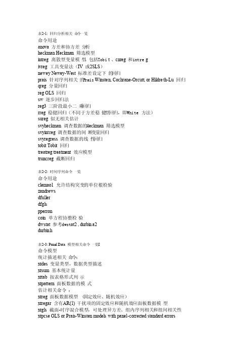
表2-1: 回归分析相关命令一览命令用途anova 方差和协方差分析heckman Heckman筛选模型intreg离散型变量模型,包括Tobit、cnreg 和intregivreg 工具变量法(IV 或2SLS)newey Newey-West 标准差设定下的回归prais 针对序列相关的P rais-W insten, Cochran e-Orcutt, or Hildret h-Lu 回归qreg 分量回归reg OLS 回归sw 逐步回归法reg3 三阶段最小二乘回归rreg 稳健回归(不同于方差稳健型回归,即White方法)sureg 似无相关估计svyheck man 调查数据的Heckman筛选模型svyintr eg 调查数据的间断变量回归svyregr ess 调查数据的线性回归tobit Tobit 回归treatre g treatme nt 效应模型truncre g 截断回归表2-2: 时间序列命令一览命令用途clemao1允许结构突变的单位根检验zandrew sdfullerdfglspperroncoin 单方程协整检验dwstat参考dwstat2 , durbina2durbinh表2-3: Panel Data 模型相关命令一览I命令模型统计描述相关命令:xtdes 变量类型,数据类型描述xtsum 基本统计量xttab 按表格形式列示xtpatte rn 面板数据的模式估计相关命令:xtreg 面板数据模型(固定效应、随机效应)xtregar含有AR(1) 干扰项的固定效应和随机效应面板数据模型xtgls 截面-时序混合模型,可处理异方差、组内序列相关和组间相关性xtpcseOLS or Prais-Winsten modelswith panel-correct ed standar d errorsxtrchhHildret h-Houck randomcoeffic ientsmodelsxtivreg面板模型的工具变量或两阶段最小二乘法估计xtabond Arellan o-Bond(1991) 线性动态面板数据模型估计xtabond2 Arellan o-Bover(1995) 系统GMM 动态面板数据模型估计xttobit Tobit 随机效应面板模型xtintre g Random-effects interva l data regress ion modelsxtlogit Fe, Re, Pa logit modelsxtprobi t Re, Pa probitmodelsxtclogl og Re, Pa cloglog modelsxtpoiss on Fe, Re, Pa Poisson modelsxtnbreg Fe, Re, Pa negativ e binomia l modelsxtfront ier 面板随机前沿模型xthtylo r Hausman-Taylorestimat or for error-compone nts models表2-4: Panel Data 模型相关命令一览II命令模型假设检验相关:test Wald 检验,如时间效应联合显著性检验xttest0随机效应检验xttest1面板序列相关检验xttest2 adsxtseria l Wooldri dge 一阶序列相关检验xtab Arellan o 面板一阶序列相关检验hausman Hausman检验面板单位根和协整相关:xtunitstata提供的检验方法ipshinIPS(2003)面板单位根检验levilin Levin,Lin和Chu(LLC, 2002)面板单位根检验madfull er Sarno-Taylor(1998) 面板单位根检验xtfishe r Maddala和Wu(1999),基于P 值的面板单位根检验表2-5: Post-estimat ion Command s命令名称用途adjust列示预测结果的均质,适于多种回归分析,可分组列示estimat es 估计结果的存储、再显示、列表比较等hausman Hausman模型识别检验lincom获得参数的线性组合,在Logit模型中可以获得系数线性组合的OR 值linktes t 但方程link识别检验,用y 对O y 和O y2 回归lrtest似然比(LR)检验mfx 计算边际效应和弹性系数nlcom 系数的非线性组合predict获得拟合值、残差等predict nl 获得非线性估计的拟合值、残差等test 线性约束的假设检验,Wald 检验testnl非线性约束的假设检验vce 列示参数估计值的方差-协方差矩阵表2-6: 二维图种类一览图形种类简单描述scatter scatter plotline line plotconnect ed connect ed-line plotscatter i scatter with immedia te argumen tsarea line plot with shadingbar bar plotspike spike plotdroplin e droplin e plotdot dot plotrarea range plot with area shadingrbar range plot with barsrspikerange plot with spikesrcap range plot with cappedspikesrcapsym range plot with spikescappedwith symbols rscatte r range plot with markersrline range plot with linesrconnec ted range plot with lines and markerstslinetime-seriesplottsrline time-seriesrange plotmband median-band line plotmspline splineline plotlowessLOWESSline plotlfit linearpredict ion plotqfit quadrat ic predict ion plotfpfit fractio nal polynom ial plotlfitcilinearpredict ion plot with CIsqfitciquadrat ic predict ion plot with CIsfpfitci fractio nal polynom ial plot with CIsfunctio n line plot of functio nhistogr am histogr am plotkdensit y kerneldensity plot表2-7: 二维图选项一览选项类别简单描述added line options draw lines at specifi ed y or x valuesadded text optiondisplay text at specifi ed (y,x) value axis options labels, ticks, grids, log scalestitle options titles, subtitl es, notes, caption slegendoptionlegendexplain ing what means what scale(#) resizetext, markers, and line widthsregionoptions outlini ng, shading, aspectratio, sizeaspectoptionconstra in aspectratio of plot regionscheme(schemen ame) overall lookby(varlist, ...) repeatfor subgrou psnodrawsuppres s display of graphname(name, ...) specify name for graphsaving(filenam e, ...) save graph in fileadvance d options difficu lt to explain表2-9: 模拟分析相关命令一览命令用途备注抽样相关:corr2da ta 产生具有指定相关性的数据仅适用于模拟相关分析drawnor minvnorm(uniform()) 产生服从标准正态分布的随机数函数,可调节均值和方差matunif orm(r,c) 产生均匀分布函数sample从现有数据中进行非重复随机抽样参考bsamplesim arma 产生服从ARI MA 过程的随机变量需要下载Bootstr ap 相关:bootstr apbsbstatbsampleMC 相关:simulat e MC simulat ionjknife类似于MCpermutepostfil e 存储MC 的结果statsbyexp list。
- 1、下载文档前请自行甄别文档内容的完整性,平台不提供额外的编辑、内容补充、找答案等附加服务。
- 2、"仅部分预览"的文档,不可在线预览部分如存在完整性等问题,可反馈申请退款(可完整预览的文档不适用该条件!)。
- 3、如文档侵犯您的权益,请联系客服反馈,我们会尽快为您处理(人工客服工作时间:9:00-18:30)。
********* 面板数据计量分析与软件实现 *********说明:以下do文件相当一部分内容来自于中山大学连玉君STATA教程,感谢他的贡献。
本人做了一定的修改与筛选。
*----------面板数据模型* 1.静态面板模型:FE 和RE* 2.模型选择:FE vs POLS, RE vs POLS, FE vs RE (pols混合最小二乘估计) * 3.异方差、序列相关和截面相关检验* 4.动态面板模型(DID-GMM,SYS-GMM)* 5.面板随机前沿模型* 6.面板协整分析(FMOLS,DOLS)*** 说明:1-5均用STATA软件实现, 6用GAUSS软件实现。
* 生产效率分析(尤其指TFP):数据包络分析(DEA)与随机前沿分析(SFA)*** 说明:DEA由DEAP2.1软件实现,SFA由Frontier4.1实现,尤其后者,侧重于比较C-D与Translog生产函数,一步法与两步法的区别。
常应用于地区经济差异、FDI 溢出效应(Spillovers Effect)、工业行业效率状况等。
* 空间计量分析:SLM模型与SEM模型*说明:STATA与Matlab结合使用。
常应用于空间溢出效应(R&D)、财政分权、地方政府公共行为等。
* ---------------------------------* --------一、常用的数据处理与作图-----------* ---------------------------------* 指定面板格式xtset id year (id为截面名称,year为时间名称)xtdes /*数据特征*/xtsum logy h /*数据统计特征*/sum logy h /*数据统计特征*/*添加标签或更改变量名label var h "人力资本"rename h hum*排序sort id year /*是以STATA面板数据格式出现*/sort year id /*是以DEA格式出现*/*删除个别年份或省份drop if year<1992drop if id==2 /*注意用==*/*如何得到连续year或id编号(当完成上述操作时,year或id就不连续,为形成panel 格式,需要用egen命令)egen year_new=group(year)xtset id year_new**保留变量或保留观测值keep inv /*删除变量*/**或keep if year==2000**排序sort id year /*是以STATA面板数据格式出现sort year id /*是以DEA格式出现**长数据和宽数据的转换*长>>>宽数据reshape wide logy,i(id) j(year)*宽>>>长数据reshape logy,i(id) j(year)**追加数据(用于面板数据和时间序列)xtset id year*或者xtdestsappend,add(5) /表示在每个省份再追加5年,用于面板数据/tsset*或者tsdes.tsappend,add(8) /表示追加8年,用于时间序列/*方差分解,比如三个变量Y,X,Z都是面板格式的数据,且满足Y=X+Z,求方差var(Y),协方差Cov(X,Y)和Cov(Z,Y)bysort year:corr Y X Z,cov**生产虚拟变量*生成年份虚拟变量tab year,gen(yr)*生成省份虚拟变量tab id,gen(dum)**生成滞后项和差分项xtset id yeargen ylag=l.y /*产生一阶滞后项),同样可产生二阶滞后项*/gen ylag2=L2.ygen dy=D.y /*产生差分项*/*求出各省2000年以前的open inv的平均增长率collapse (mean) open inv if year<2000,by(id)变量排序,当变量太多,按规律排列。
可用命令aorder或者order fdi open insti*-----------------* 二、静态面板模型*-----------------*--------- 简介 -----------* 面板数据的结构(兼具截面资料和时间序列资料的特征)use product.dta, clearbrowsextset id yearxtdes* ---------------------------------* -------- 固定效应模型 -----------* ---------------------------------* 实质上就是在传统的线性回归模型中加入 N-1 个虚拟变量,* 使得每个截面都有自己的截距项,* 截距项的不同反映了个体的某些不随时间改变的特征** 例如: lny = a_i + b1*lnK + b2*lnL + e_it* 考虑中国29个省份的C-D生产函数*******-------画图------**散点图+线性拟合直线twoway (scatter logy h) (lfit logy h)*散点图+二次拟合曲线twoway (scatter logy h) (qfit logy h)*散点图+线性拟合直线+置信区间twoway (scatter logy h) (lfit logy h) (lfitci logy h)*按不同个体画出散点图和拟合线,可以以做出fe vs re的初判断*twoway (scatter logy h if id<4) (lfit logy h if id<4) (lfit logy h if id==1) (lfit logy h if id==2) (lfit logy h if id==3)*按不同个体画散点图,so beautiful!!!*graph twoway scatter logy h if id==1 || scatter logy h ifid==2,msymbol(Sh) || scatter logy h if id==3,msymbol(T) || scatter logy h if id==4,msymbol(d) || , legend(position(11) ring(0) label(1 "北京")label(2 "天津") label(3 "河北") label(4 "山西"))**每个省份logy与h的散点图,并将各个图形合并twoway scatter logy h,by(id) ylabel(,format(%3.0f)) xlabel(,format(%3.0f))*每个个体的时间趋势图*xtline h if id<11,overlay legend(on)* 一个例子:中国29个省份的C-D生产函数的估计tab id, gen(dum)list* 回归分析reg logy logk logl dum*,est store m_olsxtreg logy logk logl, feest store m_feest table m_ols m_fe, b(%6.3f) star(0.1 0.05 0.01)* Wald 检验test logk=logl=0test logk=logl* stata的估计方法解析* 目的:如果截面的个数非常多,那么采用虚拟变量的方式运算量过大* 因此,要寻求合理的方式去除掉个体效应* 因为,我们关注的是 x 的系数,而非每个截面的截距项* 处理方法:** y_it = u_i + x_it*b + e_it (1)* ym_i = u_i + xm_i*b + em_i (2) 组内平均* ym = um + xm*b + em (3) 样本平均* (1) - (2), 可得:* (y_it - ym_i) = (x_it - xm_i)*b + (e_it - em_i) (4) /*within estimator*/ * (4)+(3), 可得:* (y_it-ym_i+ym) = um + (x_it-xm_i+xm)*b + (e_it-em_i+em)* 可重新表示为:* Y_it = a_0 + X_it*b + E_it* 对该模型执行 OLS 估计,即可得到 b 的无偏估计量**stata后台操作,揭开fe估计的神秘面纱!!!egen y_meanw = mean(logy), by(id) /*个体内部平均*/egen y_mean = mean(logy) /*样本平均*/egen k_meanw = mean(logk), by(id)egen k_mean = mean(logk)egen l_meanw = mean(logl), by(id)egen l_mean = mean(logl)gen dyw = logy - y_meanwgen dkw = logk - k_meanwgen dlw=logl-l_meanwreg dyw dkw dlw,noconsest store m_statagen dy = logy - y_meanw + y_meangen dk = logk - k_meanw +k_meangen dl=logl-l_meanw+l_meanreg dy dk dlest store m_stataest table m_*, b(%6.3f) star(0.1 0.05 0.01)* 解读 xtreg,fe 的估计结果xtreg logy h inv gov open,fe*-- R^2* y_it = a_0 + x_it*b_o + e_it (1) pooled OLS * y_it = u_i + x_it*b_w + e_it (2) within estimator * ym_i = a_0 + xm_i*b_b + em_i (3) between estimator ** --> R-sq: within 模型(2)对应的R2,是一个真正意义上的R2 * --> R-sq: between corr{xm_i*b_w,ym_i}^2* --> R-sq: overall corr{x_it*b_w,y_it}^2**-- F(4,373) = 855.93检验除常数项外其他解释变量的联合显著性 ***-- corr(u_i, Xb) = -0.2347**-- sigma_u, sigma_e, rho* rho = sigma_u^2 / (sigma_u^2 + sigma_e^2)dis e(sigma_u)^2 / (e(sigma_u)^2 + e(sigma_e)^2)** 个体效应是否显著?* F(28, 373) = 338.86 H0: a1 = a2 = a3 = a4 = a29* Prob > F = 0.0000 表明,固定效应高度显著*---如何得到调整后的 R2,即 adj-R2 ?ereturn listreg logy h inv gov open dum**---拟合值和残差* y_it = u_i + x_it*b + e_it* predict newvar, [option]/*xb xb, fitted values; the defaultstdp calculate standard error of the fitted values ue u_i + e_it, the combined residualxbu xb + u_i, prediction including effectu u_i, the fixed- or random-error componente e_it, the overall error component */xtreg logy logk logl, fepredict y_hatpredict a , upredict res,epredict cres, uegen ares = a + reslist ares cres in 1/10* ---------------------------------* ---------- 随机效应模型 ---------* ---------------------------------* y_it = x_it*b + (a_i + u_it)* = x_it*b + v_it* 基本思想:将随机干扰项分成两种* 一种是不随时间改变的,即个体效应 a_i* 另一种是随时间改变的,即通常意义上的干扰项 u_it* 估计方法:FGLS* Var(v_it) = sigma_a^2 + sigma_u^2* Cov(v_it,v_is) = sigma_a^2* Cov(v_it,v_js) = 0* 利用Pooled OLS,Within Estimator, Between Estimator* 可以估计出sigma_a^2和sigma_u^2,进而采用GLS或FGLS* Re估计量是Fe估计量和Be估计量的加权平均* yr_it = y_it - theta*ym_i* xr_it = x_it - theta*xm_i* theta = 1 - sigma_u / sqrt[(T*sigma_a^2 + sigma_u^2)]* 解读 xtreg,re 的估计结果use product.dta, clearxtreg logy logk logl, re*-- R2* --> R-sq: within corr{(x_it-xm_i)*b_r, y_it-ym_i}^2* --> R-sq: between corr{xm_i*b_r,ym_i}^2* --> R-sq: overall corr{x_it*b_r,y_it}^2* 上述R2都不是真正意义上的R2,因为Re模型采用的是GLS估计。