瑞典山高节拍计算书

合集下载

selberg公式

selberg公式
Selberg公式是一个数学公式，用于计算特定条件下的临界风速，以避免风致振动现象（颤振）的发生。

颤振是一种振幅不断增大的振动，可能导致结构的损坏。

这个公式中，扭弯频率比越大，颤振临界风速越高；质量（质惯矩）越大，颤振临界风速也越高。

扭弯频率比和质量（质惯矩）是与结构本身相关的参数。

需要注意的是，颤振的发生与多种因素有关，包括结构的形状、质量、刚度、阻尼以及风速、风向等外部条件。

在实际工程中，需要通过详细的分析和计算来确定颤振的临界风速，并采取相应的措施来避免颤振的发生，确保结构的安全和稳定。

关于该公式具体的操作，需要请专业的工程师来计算和应用，请谨慎参考。

108钢管抗风柱高度16m计算书

108钢管抗风柱高度16m计算书一、背景与目的108钢管抗风柱是作为建筑物或其他工程结构的支撑构件，用于抵抗风力对建筑物的影响。

针对某工程项目中使用的108钢管抗风柱高度为16m，本文旨在对其进行详细的计算和分析，以确保其在实际使用中的安全和稳定性。

二、计算基本参数1. 钢管型号：1082. 抗风柱高度：16m3. 风载荷标准：GBxxx-2012《建筑结构荷载规范》4. 钢管材质：Q2355. 抗风柱使用环境：____（根据实际情况填写）三、风荷载计算1. 确定风载荷标准：根据《建筑结构荷载规范》，结合工程实际情况确定抗风柱所在地的风荷载标准。

2. 计算风荷载大小：根据所在地风载荷标准和抗风柱高度，计算抗风柱受到的风荷载大小。

四、结构稳定性计算1. 确定抗风柱所受风荷载情况下的受力情况：根据风荷载大小和抗风柱结构特点，确定抗风柱所在风场下的受力情况。

2. 结构稳定性分析：根据受力情况，进行抗风柱的结构稳定性分析，包括受力点弯矩、剪力等参数的计算和分析。

五、材料强度计算1. 确定使用材料的强度参数：根据抗风柱所使用的钢管型号和材质，确定其材料的强度参数。

2. 材料强度验证：根据实际受力情况和材料参数，验证抗风柱材料的强度是否满足要求。

六、结论与建议1. 结论：根据以上计算和分析结果，得出抗风柱在16m高度下的结构稳定性和材料强度都满足使用要求。

2. 建议：在实际使用中，需要注意抗风柱的安装、连接及固定等细节，确保其在实际使用中的安全性和稳定性。

七、附录（可以包括相关计算公式、数据表格、图纸等）通过以上计算书的编写，可以全面、客观地展现出对108钢管抗风柱16m高度的计算和分析过程，为实际工程应用提供参考依据，确保抗风柱在使用中的安全和稳定。

六、结论与建议1. 结论：根据以上计算和分析结果，得出抗风柱在16m高度下的结构稳定性和材料强度都满足使用要求。

在考虑风载荷和材料强度的情况下，抗风柱能够有效地抵抗风力对建筑物或其他工程结构的影响。

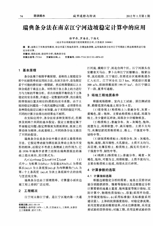
瑞典条分法在南京江宁河边坡稳定计算中的应用

６结论
通过对江宁河堤防稳定进行分析，整个断从面的稳定计算结果来看，各种工况下计算得到的稳定安全系数均能够满足规范要求。我们认
图１背水坡最危险滑动面及其安全系数计算结果图《稳定渗流期）
９５Ｏ
５
１ ∞
Ｊ
ｌ
５
参照《防工程设计规范》堤防边坡抗滑稳堤，定计算可分为正常情况和非常情况两种工况。本工程为对原有堤防加固工程，身已固结稳定，堤因此不对非常情况的施工期的迎水坡、背水坡稳定抗滑进行计算。
最危险滑动面及安全系数计算结果图。背水坡抗滑稳定计算（稳定渗流期）安全系数为１８，．７满５足容许安全系数１１．５的要求；迎水坡抗滑稳定计算（位骤降期）全系数为１０，足容许安水安．６满９全系数１１．５的要求。图３图４分别为非常情况下背水坡、水坡、迎最危险滑动面及安全系数计算结果图。背水坡抗滑稳定计算（地震工况）安全系数为１０，．６满足６容许安全系数１０．５的要求；水坡抗滑稳定计算迎（震工况）安全系数为１３８地．１，满足容许安全系数１５的要求。．０
作者简介：甲存（９９，，苏南京人，徐１７一）男江工程师，事岩从土工程勘察、设计工作。

高塔基础计算书（手算）

高塔基础计算书（手算）基本计算资料：采用现行国家有关规范<<石油化工塔型设备基础设计规范>>,（SH 3030-1997）<<建筑结构荷载规范>>（GB50009-2001）<<建筑地基基础设计规范>>（GB50007-2002）<<建筑抗震设计规范>>（GB50011-2001）<<高耸结构设计规范>>（GBJ135-90）<<构筑物抗震设计规范>>（GB50191-93）<<化工设备基础设计规定>>参考手册：〈〈高塔基础设计手册〉〉以塔401为例：计算如下：一、塔设备内径：D1=2.2m, 外径：D2=2.224m塔设备高度：30m基本风压：0.5kN/ m2㎡㎡地震烈度：7度，设计地震基本加速度：0.15g。

基础置于砾石层上，地基承载力特征值:f a=400kPa。

二、荷载空塔自重：22吨，生产时操作重：31吨充水水重：110吨，平台梯子重：7吨(含管道、保温等)三、周期计算：δ1＜＝30，当h2/D2=302/2.224=404.7<700T1=0.35+0.85x10-3x h2/D2 =0.694s四、风荷载计算：w k=βz u s u z u r(1+u e)(D2+2δ2)w0u s=0.6, u r=1.1, u e=0.23, δ2=0.3w k=0.6x1.1x1.23βz u z w0 D2=0.812βz u z w0 (D2+2δ2)离地面高度H(m) 10 20 30u z 1.0 1.25 1.42u z w00.5 0.625 0.71βz 1.35 1.82 2.23w k 1.55 2.6 3.6注：βz是按高耸结构设计规范计算作用在基础顶面的剪力：Q=[1.55+(1.55+2.6)/2+(2.6+3.6)/2]x10=67kN作用在基础顶面的弯矩：M=[1.55x5+1.55x15+2.6x25+0.5x16.7x1.05+0.5x26.7x1]x10 =1180kN.m五、地震作用计算：G eq=31x10=310kNa1=(T g/T1) 0.9xa max=(0.35/0.694) 0.9x0.12=0.065F EK=a1xG eq=0.065x310=20.15kN作用在基础顶面的剪力：Q=F EK=20.15kN作用在基础顶面的弯矩：M=Qx2h/3=20.15x2x30/3=806 kN.m六、基础设计〈一〉、正常操作情况下的荷载标准组合假设基础直径5.2m，基础埋深3.0m,基础高出地面0.3m。

(一)瑞典圆弧法

二维边坡稳定分析（一）瑞典圆弧法又称为瑞典法，普通条分法，一般条分法，费伦纽斯法（Ordinary or Fellenius method）。

1简化条件仅适用圆弧滑裂面；假定每一土条侧向垂直面上的作用力平行于土条底面（亦有认为是忽略土条两侧的作用力），此假定会使牛顿“作用力等于反作用力”的原理在两个土条之间得不到满足；2坐标系和条块受力分析①坐标系规定：滑坡体位于坐标系原点的右侧即 x ≥ 0yR②典型条块受力分析（Ⅰ）条块高度为i h ,宽度为i b ,底滑面长度为i l ，底滑面倾角为i α；（Ⅱ）条块自重为i W ；（Ⅲ）地震力i c W K ，c K 为地震影响系数；（Ⅳ）作用于条块底部滑裂面的有效法向力i N '；（Ⅴ）作用于条块底部滑裂面孔隙水压力的合力i i u i W U αγsec =，u γ为孔隙水压力系数；（Ⅵ）作用于条块底部的剪切力i S ；（Ⅶ）作用于条块界面条间力的合力i i P P 1-,平行于土条底部滑裂面；（Ⅷ）作用于条块顶部的外部荷载iy Q Q ix ，作用点（pi y x pi ）。

③ 条块参数取值及符号约定（Ⅰ）条块底滑面倾角i α定义条块底滑面为矢量，方向与滑体滑动方向相反，定义该矢量与正x 轴的夹角为条块底滑面倾角i α，逆时针为正( 为负值 )i αif (12x x ≥) )arcsin(12ly y i -=α else i α落在二三象限，方法同垂直条分法求解（则212212)()(y y x x l -+-=）注意：一般情况下，i α取值范围为（2,2ππ-），滑面1→2落在一、四象限；特殊情况，如滑面1→2落在二、三象限，则无法利用垂直条分法求解，此时滑面不再是单值曲线，垂直条块界面和底滑面存在二个及以上的交点，因此程序设计时要进行数据合理性检验。

（Ⅱ）水平、竖直方向荷载在条块底部滑面法线及切线方向投影水平荷载x F ：在法线方向投影 ix i x xn F F F ααπsin )2cos(-=+=在切线方向投影i x xs F F αcos =②竖直方向荷载y F ：1212在底滑面法线方向投影i y F F αcos y n =在底滑面切线方向投影i y ys F F αsin =适用于[]ππα,-∈i ，1→2属于1、2、3、4象限均可。

计算书(LTpb)

（4）板底20厚纸筋灰粉刷16x0.02x1=0.32 KN/m
合计：4.08 KN/m
荷载设计值为：1.2x4.08+1.4x2.0=7.70KN/m
1双向板：B-1
1．1基本资料
1．1．1工程名称：五洲太阳城
1．1．2边界条件（左端/下端/右端/上端）：固端/固端/固端/固端
1．1．3荷载标准值
My'＝Max{My'(L), My'(D)}＝Max{-1.17, -1.14}＝-1.17kN·m
My'k＝-0.93kN·m My'q＝-0.75kN·m
Asy'＝104mmρ＝0.19%ρmin＝0.24% Asy'*＝189mm
φ8@200（As＝251）ωmax＝0.020mm
1．3跨中挠度验算
Bs＝Es * As * ho ^ 2 / [1.15ψ+ 0.2 + 6 *αE *ρ/ (1 + 3.5γf')]
＝210000*251*55^2/[1.15*0.200+0.2+6*8.26*0.00457/(1+3.5*0.000)]
＝243.17kN·m
设计人签字
算书应书写清楚，不得采用铅笔书写，不得随意涂改，设计人员应每张签字
φ8@200（As＝251）ωmax＝0.004mm
1．2．2平行于Ly方向的跨中弯矩My
Mygk1＝(0.03931+0.2*0.00463)*4.10*1.360^2＝0.31kN·m
Myqk1＝(0.03931+0.2*0.00463)*2.00*1.360^2＝0.15kN·m
My＝Max{My(L), My(D)}＝Max{0.57, 0.56}＝0.57kN·m

Ch03p

Chapter 3Exercise SolutionsEX3.1 ()1 , 3 , 4.5 4.531 2 TN GS DS DS DS GS TN V V V V V VV V sat V V V ====>=−=−=Transistor biased in the saturation region()()2220.8310.2 /D n GS TN n n I K V V K K mA V =−⇒=−⇒=(a) V GS = 2 V, V DS = 4.5 V Saturation region:()()20.2210.2 D D I I mA =−⇒=(b) V GS = 3 V, V DS = 1 V Nonsaturation region:()()()()20.2231110.6 D D I I mA ⎡⎤=−−⇒=⎣⎦EX3.2() 2 , 3 32 1 TP SG SD SG TP V V V VV sat V V V=−==+=−=(a) 0.5 Nonsaturation SD V V =⇒(b) 2 Saturation SD V V =⇒ (c) 5 SaturationSD V V =⇒EX3.3()()()212216010 3.636 1602800.253.63620.669 mAG DD GSD R V V V V R R I ⎛⎞⎛⎞====⎜⎟⎜⎟++⎝⎠⎝⎠=−= ()()()()100.66910 3.31 V0.669 3.31 2.21 mW DS D DS V P I V =−====EX3.4()()2211221.20.4 1.2 2.932 V 1DQ P SG TP SG SG SG DDTTN DD I K V V V V R V V V V R R R =+=−⇒=⎛⎞==⋅−⎜⎟+⎝⎠ Note K = k Ω()()2211112.93220010682 K682200283 K6821045 K 1.2D R R R R R R =⇒==⇒=+−==EX3.5(a) ()()21240105105 1 V 4060G R V R R ⎛⎞⎛⎞=−=−=−⎜⎟⎜⎟++⎝⎠⎝⎠()()25−−==−=−S D n GS TN SS G GSV I K V V R V V V()()()()()()()()2222510.51210.5 3.507 2.646 V0.5 2.6461 1.354 mA 10 1.3543 5.937 VGS GSGS GS GS GS D D DS V V V V V V I I V −−=−+−====−⇒==−=(b) ()()241GS n GS TN V K V V −=−()()()()()()()()(1) 1.050.50.525(2)0.950.50.475(3) 1.051 1.05 V (4)0.9510.95 Vn n TN TN K K V V ========(1)-(3)()2240.525 2.1 1.10250.5250.1025 3.4210 2.652 VGS GSGS GSGS GS V V V V V V −=−+−−===()()()20.5252.652 1.05 1.348 mA10 1.3483 5.957 V D DS I V =−==−=(2)-(4)()()2240.475 1.90.90250.4750.0975 3.571300.097520.475GS GS GS GS GS GS V V V V V V −=−++−=−±+=2.641 V GS V =()()()20.4752.6410.95 1.359 mA10 1.3593 5.924 V D DS I V =−==−=(1)-(4)()()224052519090250525 00025352620GS GS GS GS GS V .V .V ..V .V .−=−++−=25893 VGS V .=()()()2052525893095141110357678 VD DS D I ....V I .=−==−=(2)-(3)()2240.475 2.1+1.10250.4750.0025 3.47630GS GS GS GS GS GS V V V V V V −=−+−=22.7027(0.475)(2.7027 1.05) 1.2973 mA 10(3) 6.108 VGSD DS D V I V I ==−==−= 1.297 1.411 mA5.7686.108 V DQ DS I V ≤≤≤≤EX3.6()()()2121052001050714 V 3505512G S D S D R V R R .V I R .I ⎛⎞=−⎜⎟+⎝⎠⎛⎞=−=⎜⎟⎝⎠=−=− So()()5120714428612=−=−−=−SG S G D DV V V .I (I)()2428612−==+SGD D p SG TP .V I .I K V V()()()()()()2224286120252114286030603−=×−−+−−=−+SG SG SG SG SG SG .V ..V V .V .V .V .2030439860SG SG SG .V .V .V +−=Must use sign 304 V SG V .+⇒= ()()()()()()2025******* mA1010104124459 V , Yes D D SD D S D SD SD SD I ..I .V I R R ..V .V V sat =−⇒==−+=−+⇒=>EX3.7()()()21010SD DQ S P SD P SG TP S P V I R R V K V V R R =−+=−++Set SD SG TP V V V =+()()()2100.25 5.2+=−+SG TP SG TP V V V V()()21.3100+++−=SG TP SG TP V V V V() 2.415 VSG TP V V +==()3.415 V3.42 V SG V =()()()22.415 V 2.42 V 0.25 2.415 1.46 mASD D V I ===EX3.8()()2122401051052402700.294 V G G R V R R V ⎛⎞⎛⎞=−=−⎜⎟⎜⎟++⎝⎠⎝⎠=−()()()()()22550.084.7064 3.9 2.4 1.442S G GS D n GS TN SSGS GS GS V V V I K V V R R V V V −−−+===−⎛⎞−=−+⎜⎟⎝⎠20.6240.4976 3.807440GS GS V V −−=2.90 VGS GS V V = ()()()20.084 2.90 1.20.463 mA 210 3.910 3.57 V D D DS D DS I I V I V ⎛⎞=−⇒=⎜⎟⎝⎠=−+⇒=EX3.9()210 and SG D D p SG TP SV I I K V V R −==+()()20.120.0500.82.35 VSG SG V V =−= 10 2.3563.75 k 0.12S S R R −=⇒=Ω ()()()()()()8208200.1263.750.12200.1263.75836.25 k 0.12==−+=−−−−=⇒=ΩSD D S D D D D V I R R R R R()()()()()()()2(1)0.05 1.050.0525(2)0.050.950.0475(3)0.81.050.84 V(4)0.80.950.76 V 10P P TP TP SG DP SG TP SK K V V V I K V V R =====−=−=−=−−==+(1)-(3)()()221063.750.0525 1.680.70563.347 4.6237.63840SG SG SG SGSG V V V V V ⎡⎤−=−+⎣⎦−−=()4.62323.3472.352 V 0.120 mA 8.0 V SG SG D SD V V I V ±+==⇒≅≈ (2)-(4)()()221063.750.0475 1.520.57763.028 3.6038.2510SG SG SG SGSG V V V V V ⎡⎤−=−+⎣⎦−−=()3.60323.0282.35 V 0.1208.0SG SG D SD V V I V ±+==≈≈(1)-(4)()()221063.750.0525 1.520.57763.347 4.0878.066850SG SG SG SGSG V V V V V ⎡⎤−=−+⎣⎦−−=2.279 V 0.121 mA7.89 V SG SG D SD V V I V ====(2)-(3)()()221063.750.0475 1.680.70563.028 4.08737.86340SG SG SG SGSG V V V V V ⎡⎤−=−+⎣⎦−−=()4.087323.0282.422 V 0.119 mA 8.11 VSG SG D SD V V I V ±+====Summary 01190121 mA789811 VD SD .I ..V .≤≤≤≤EX3.10()()()()()()22222,10100.22102882720Use Power 0.623 3.77Power 2.35 mW DDGS D D n GS TN SGS GS GS TN TN GS GS GS GSGS GS D D DS V V I I K V V R V V V V V V V V V V V I I V −==−−=−+−=−+−−===⇒=EX3.11(a) 4 V, I V =Driver in Non ⋅ Sat.()[]()()()222222225241514168638160nD I TND O O nL DD O TNL D D D O O O D O K V V V V K V V V V V V V V V V V ⎡⎤−−=−−⎣⎦⎡⎤−−=−−=−=−+⎣⎦−+= 0.454 VD D V V = (b) 2 V I V =Driver: Sat[][][][]222252151nD I TND nL DD O TNL O K V V K V V V V −=−−−=−−4 1.76 V O O V V =−⇒=EX3.12If the transistor is biased in the saturation region()()()()()()()2220.25 2.5 1.56 mA10 1.564 3.753.75 2.5D n GS TN n TN D D DS DD D S DS DS GS TN TN I K V V K V I I V V I R V V V V V =−=−=⇒==−=−⇒=>−=−>−− Yes — biased in the saturation region()()Power 1.56 3.75Power 5.85 mW D DS I V ==⇒=EX3.13 (a) For V I = 5 V , Load in saturation and driver in nonsaturation. ()()()()()22222510.250.254 2.06DD DLnD I TND O O nL TNL nD nD nL nLI I K V V V V K V K K K K =⎡⎤−−=−⎣⎦⎡⎤−−=⇒=⎣⎦(b)()()22220.2250 / and 103 /DL nL TNL nL nL nD I K V K K A V K A Vμμ=−⇒=−−⎡⎤⎣⎦==EX3.14 ()()()()22For 15 3.251 1.75 sat 1.7510.75 V =−=+=+−−====−⇒=NDN DPn GSN TN p scop TP GSN I o DSN o M I I K V V K V V V V V V V V()()For : 1.75 Vsat 5 3.2510.75 V So 50.75 4.25 V=−==+=−−==−⇒=P I DD O SD SGP TP ot ot M V V V V V V V VEX3.15For 10 ,D R k =Ω V DD = 5 V , and V o = 1 V()()()()()()222510.4 1020.4251110.057 /0.410.4 D D n GS TN DS DS D n n D DS I mA I K V V V V I K K mA V P I V P mW−==⎡⎤=−−⎣⎦⎡⎤==−−⇒=⎣⎦=⋅=⇒=EX3.16a. 12225 V,0, cutoff 0D V V M I ==⇒= ()()()()22000520.05302515O D n I TN O O D V I K V V V V R V V V −⎡⎤=−−=⎣⎦⎡⎤−−=−⎣⎦20001.51350R V V V I −+===b.12 5 V ==V V(){}()()()22000200522520.0530********On I TN O O DV K V V V V R V V V V V −⎡⎤=−−⎣⎦⎡⎤−=−−⎣⎦−+=EX3.172311& watched 0.4 mA ⇒==Q REF M M I I ()()23322110.40.31 2.15 V0.40.61 1.82 VGS GS GS GS GS V V V V V =−⇒===−⇒=EX3.18()()()()()2220.040.1150.621.177 0.040.2 1.1770.62300.040.2250.62 1.23 V SGC SGC SGBBB SGA SGA V V V V W L W L V V ⎛⎞=−⎜⎟⎝⎠==⎛⎞⎛⎞=−⎜⎟⎜⎟⎝⎠⎝⎠⎛⎞=⎜⎟⎝⎠⎛⎞=−⎜⎟⎝⎠=EX3.19(a)()()()()223344342244332 3 121314=−=−=⇒=−=−⇒=REF n GS TN n GS TN GS GS n n n n I K V V K V V V V V VK K K K (b) ()()222232222But 20.1210.1 /=−===−⇒=Q n GS TN GS GS n n I K V V V V V K K mA V(c) ()()223322440.2210.2 /0.2310.05 /n n n n K K mA V K K mA V =−⇒==−⇒=EX3.20()()222222222222555016.7 K 0.30.30.2 1.2 2.425 V 2.425 VS S D n GS TN GS GS G GS S V R I K V V V V V V V =−====−=−⇒=⇒=+=15 2.42525.8 K 0.1D R −== ()()()()()()12111211112111111211212.4255 2.575 V 2.575524.3 K0.10.10.5 1.2 1.647 V 1.647 2.5750.928 V1105105S G DSQ S S D n GS TN GS GS G GS S G G TN V V V R R I K V V V V V V V V R V R R R R =−=−=−−−−=⇒==−=−⇒==+=+−⇒=−⎛⎞=−=⋅⋅−⎜⎟+⎝⎠()()1122210.928200105491 K491 200337 K491R R R R R −=−⇒==⇒=+EX3.211221111113313123211225(0.25)(16)5 1 V()0.250.5(0.8) 1.507 V 1.50710.507 V(5)0.507(5)50.7 K 5001 2.5 1.5 V 1.5 1.507S D S DQ n GS TN GS GS G GS S G S S DS G S GS V I R I K V V V V V V V R R V R R R R V V V V V V =−=−=−=−⇒=−⇒==+=−=⎛⎞=⇒=⇒=⎜⎟++⎝⎠=+=−+==+=+23232123 3.007 V(5) 3.007(5)500G R R R R V R R R =⎛⎞++⎛⎞=⇒=⎜⎟⎜⎟++⎝⎠⎝⎠2322300.7300.750.7250 K R R R R +==−⇒=1122250025050.7199.3 K 1.5 2.5 4 V 544 K 0.25D S DS D D R R V V V R R =−−⇒==+=+=−=⇒=EX3.22()()()()()22sat 1.2 4.5sat 3.3 V1.21121 6.45 mA 4.5DS GS P DS GS D DSS D P V V V V V I I I V =−=−−−⇒=⎛⎞−⎛⎞=−=−⇒=⎜⎟⎜⎟⎜⎟−⎝⎠⎝⎠EX3.23Assume the transistor is biased in the saturation region.()()()()()2218181 1.17 V 1.173.51580.88.68.6 1.177.43 V7.43 1.17 3.5 2.33GS D DSS P GS GS S GS D DS DS GS P V I I V VV V V V V V V V ⎛⎞=−⎜⎟⎝⎠⎛⎞=−⇒=−⇒=−=⎜⎟⎜⎟−⎝⎠=−==−==>−=−−−=Yes, the transistor is biased in the saturation region.EX3.24 ()()()()22212122122.5 mA 12.561 1.42 V45 2.50.2554.37566 4.375 1.62551625 1.35 k 2.5202200 k 1.42 4.375 5.795D GS D DSS P GS GS S D S S DS D D D G GS S G I V I I V V V V I R V V V R R R R R R V V V R V R R =⎛⎞=−⎜⎟⎝⎠⎛⎞=−⇒=−⎜⎟⎜⎟−⎝⎠=−=−=−=⇒=−=−=⇒=Ω=⇒+=Ω+=+=−−=−⎛=⎜+⎝()()22120105.795201042.05 k 42 k 200157.95 k 158 k R R R ⎞−⎟⎠⎛⎞−=−⇒=Ω→Ω⎜⎟⎝⎠=Ω→ΩEX3.2522220.16161142160.375460S GSS GS D S SGS D DSS P GS GS GS GS GS GS V V V V I R R V I I V V V V V V V −=−==⎛⎞=−⎜⎟⎝⎠⎛⎞⎛⎞=−=−+⎜⎟⎜⎟⎝⎠⎝⎠−+=()()()()05 1.810.45 4.2781.81 4.276 2.47 V sat 4 1.81 2.19D D D SD S SD SD P GS V I R V V V V V V V =−=−=−=−=−−−⇒==−=−=()So sat SD SD V V >EX3.26()()121212100 k 5 mA,5 1.2 6 V 12 V in DQ S DQ S SDQ D S SDQR R R R R R R I V I R V V V V ===Ω+==−=−=−=⇒=−& 61218 V =−−=−()()2221218200.4 k 5158140.838 V0.8386 5.16220D D GS GS DQ DSS P GSG GS S G R R V V I I V V V V V R V R R −−−=⇒=Ω⎛⎞⎛⎞=−⇒=−⎜⎟⎜⎟⎝⎠⎝⎠==+=−=−⎛⎞=−⎜⎟+⎝⎠()()()()()()()111222122215.16210020387 k 100387100387100 387100100387135 k R R R R R R R R R R −=−⇒=Ω=⇒=++−=⇒=ΩTYU3.1(a) () 1.2 , 2 2 1.20.8 ===−=−=TN GS DS GS TN V V V V V sat V V V(i) 0.4 Nonsaturation DS V =⇒ (ii) 1 Saturation DS V =⇒ (iii) 5 Saturation DS V =⇒ (b) ()()1.2 , 2 2 1.2 3.2 =−==−=−−=TN GS DS GS TN V V V V V sat V V V(i) 0.4 Nonsaturation DS V =⇒ (ii) 1 Nonsaturation DS V =⇒ (iii) 5 Saturation DS V =⇒TYU3.2(a) ()()()()()()1488822 3.98.85107.6710 /450101005007.67100.274 /27μ−−−−=×∈===×××=⇒=n oxn ox ox ox n n W C K LC F cm t K K mA V(b) V TN = 1.2 V, V GS = 2 V(i)()()()()20.4 Nonsaturation0.27422 1.20.40.40.132 =⇒⎡⎤=−−⇒=⎣⎦DS D D V V I I mA(ii) ()()21 Saturation0.2742 1.20.175 =⇒=−⇒=DS D D V V I I mA(iii) ()()25Saturation 0.2742 1.20.175 1.2 , 2 =⇒=−⇒==−=DS D D TN GS V V I I mAV V V V(i)()()()()20.4 Nonsaturation0.27422 1.20.40.40.658 DS D D V V I I mA=⇒⎡⎤=+−⇒=⎣⎦(ii) ()()()()21Nonsaturation 0.27422 1.211 1.48 DS D D V V I I mA=⇒⎡⎤=+−⇒=⎣⎦(iii) ()()25 Saturation0.2742 1.2 2.81 =⇒=+⇒=DS D D V V I I mATYU3.3(a) (sat)21208V SD SG TP V V V ..=+=−=(i) Non Sat (ii) Sat (iii) Sat(b) (sat)21232 V SD V ..=+=(i) Non Sat (ii) Non Sat (iii) SatTYU3.4 (a)()()14p ox ox 8882C (3.9)(8.8510)C 350109.861103009.86110(40)(2)20.296/P P P W K L Z K K mA Vμ−−−−⎛⎞×⎛⎞==⎜⎟⎜⎟×⎝⎠⎝⎠=×⎛⎞×⎜⎟=⎜⎟⎝⎠= (b)(i) 2(0.296)2(2 1.2)(0.4)(0.4)0.142 mA⎡⎤=−−⎣⎦=D I(ii) []2(0296)2120189 mA D D I ..I .=−⇒= (iii) I D = 0.189 mA(i) ()()()2(0296)221204040710 mA⎡⎤=+−⎣⎦=D I .....(ii) ()()()2(0296)221211=1.60 mA⎡⎤=+−⎣⎦D I ..(iii) ()()2029******* mA=+=D I ...TYU3.5(a) ()()()20, 2.50.8 1.7 For 2 , 10 Saturation Region0.1 2.50.80.289 λ==−===⇒=−⇒=DS DS DS D D V sat V V V V V I I mA(b) ()()()()()()()()()()()12220.02 1For 2 0.1 2.50.810.0220.300 10 0.1 2.50.810.02100.347 λλ−==−+==−+⇒=⎡⎤⎣⎦=⎡⎤=−+⇒=⎣⎦D n GS TN DS DS D D DS D D V I K V V V V VI I mA V VI I mA(c) For part (a), 0o r λ=⇒=∞For part (b), 10.02 ,V λ−= ()()()()11220.020.1 2.50.8o n GS TN r K V V λ−−⎡⎤⎡⎤=−=−⎣⎦⎣⎦ or 173 o r k =ΩTYU3.620.70 ,1TN TNO f TNO V V V V Vγφ=+==(a) 0, 1 SB TN V V V =⇒=(b) ()1 ,10.35 1.16 SB TN TN V V V V V ==+⇒= (c) ()4 ,10.35 1.47SB TN TN V V V V V ==+⇒=TYU3.7()()()222122210.40.250.8 2.06 V 2.067.568.8 k 250181.2 k 47.548.75 k 0.4D n GS TN GS GS GS DDDS DD D DD D I K V V V V R V V R R R R R V V I R R R =−=−⇒=⎛⎞=⎜⎟+⎝⎠⎛⎞=⇒=Ω⎜⎟⎝⎠=Ω==−−=⇒=Ω(), Yes DS DS V V sat >TYU3.8()()()()()225 and 5So 0.10.10.080 1.2 2.32 V5 2.32So 26.8 k 0.1 4.5 2.322.1855 2.1828.2 k 0.1, YesS D S GSS GS S D n GS TN GS GS S S DS D S D DS S D D D D D DS DS V I V V R V R I K V V V V R R V V V V V V V V R R I V V sat −−==−−==−=−⇒=−=⇒=Ω=−⇒=+=−=−−==⇒=Ω>TYU3.9()()()()()22For 2.2 5 2.20.56 50.56 2.210.389 /2389219.440DS D D D n GS TN n n oxn V VI I mA I K V V K C W K mA V LW WL L =−=⇒==−=−==⋅=⇒=μTYU3.10(a)The transition point is15111−+=−++==DD TNL TND It V V V V V(b) We may write()()()220.05 2.236176.4 D nD GSD TND D I K V V I A μ=−=−⇒=TYU3.11151112.55 2.52.55 1.67 2.781.5−+=−++=−+=⇒==⇒/=DD TNL TND It nD nL V V V V K Kb. For V I = 5, driver in nonsaturated region.()()()[]()[]()222222000220002002000222.782515122.24 2.7841683.7830.24160DD DLnD I TND O O nL GSL TNL nD I TND O O DD O TNL nLI I K V V V V K V V K V V V V V V V K V V V V V V V V V V V =⎡⎤−−=−⎣⎦⎡⎤−−=−−⎣⎦⎡⎤−−=−−⎣⎦−=−=−+−+==TYU3.12We have 1.2 1.8 DS GS TN TN V V V V V V =<−=−= Transistor is biased in the nonsaturation region.()()()()()()()()2225 1.22 and 0.475 80.47520 1.8 1.2 1.20.475 2.880.165 216529.4335μ−−⎡⎤=−−==⇒=⎣⎦⎡⎤=−−−⎣⎦=⇒=/=⋅=⇒=DD DS D n GS TN DS DS D D Sn n n n oxn V V I K V V V V I I mA R K K K mA V C W K LW W L LTYU3.13(a)Transition point for the load transistor – Driver is in the saturation region. ()()())222 12 1.89 =−=−=−=−⇒=−=−=⇒=DD DL nD GSD TND nL GSL TNL DSL GSL TNL TNL DSL DD Ot It It I I K V V K V V V sat V V V V V V V V V V(b) For the driver: 1.89 , 0.89 Ot It TNDIt Ot V V V V V V V =−==TYU3.14()()()()()2220.0502100.70.350.350.319 mA100.3530.3 k 0.319D n GS TN DS DS D DD o D D D I K V V V V I V V R R I ⎡⎤=−−⎣⎦⎡⎤=−−⎣⎦=−−==⇒=ΩTYU3.15(a) Transistor biased in the nonsaturation region()()2225 1.5122124250.8433.6120 0.374 DSD D n GS TN DS DS DS DS DS DS DS V I RI K V V V V V V V V V V−−==⎡⎤=−−⎣⎦⎡⎤=−−⎣⎦−+=⇒=Then 5 1.50.374261 12R R −−=⇒=ΩTYU3.16a.()()()()()22225250.102510.100.100.248 /25−⎡⎤==−−⎣⎦−⎡⎤=−−⇒=⎣⎦OD n TN O O Dn n V I K V V V V R K K mA Vb.()()200020002000520.24825125512.4812.4100.250V V V V V V V V V −⎡⎤=−−⎣⎦⎡⎤−=−⎣⎦−+==TYU3.17()()()()()()225500.150.466 V0.005100.050 V 0.4660.0500.516 V 50.005100 4.5 V 4.50.050 4.45 VDQ GS TN GS GS S GG GS S GG D D DS D S DS I K V V V V V V V V V V V V V V V =−⇒=−⇒===⇒=+=+⇒==−⇒==−=−⇒=TYU3.18()()()()22210020.70.20.10.19 A 2.50.1267 k 0.009D GS TN DS DS D D D I K V V V V I R R μ⎡⎤=−−⎣⎦⎡⎤=−−⎣⎦=−=⇒=Ω。

超高斜坡高度计算公式

超高斜坡高度计算公式在工程建设和地质勘探中，经常会遇到需要计算超高斜坡高度的情况。

超高斜坡是指坡度非常陡峭的山坡或者悬崖，其高度计算需要特殊的公式和方法。

本文将介绍超高斜坡高度计算的公式和相关知识，希望能对工程建设和地质勘探工作者有所帮助。

超高斜坡高度计算的公式主要依赖于坡度和坡角。

坡度是指斜坡上升或下降的程度，通常以百分比或者角度表示。

坡角则是指斜坡与水平面的夹角。

在实际的工程测量中，我们常常会遇到需要通过坡度和坡角来计算超高斜坡高度的情况。

首先，我们来看一下超高斜坡高度计算的基本公式。

假设斜坡的坡度为S，坡角为α，则超高斜坡的高度H可以通过以下公式计算得出：H = L S。

其中，L为斜坡的水平距离。

这个公式的推导过程比较简单，可以通过几何关系和三角函数来进行推导。

在实际应用中，我们可以根据这个公式来计算超高斜坡的高度，从而为工程建设和地质勘探提供参考数据。

然而，这个公式只适用于坡度较小的情况，对于超高斜坡来说，坡度往往会非常陡峭，这时候就需要考虑坡角对高度的影响。

在这种情况下，我们需要引入坡角来修正超高斜坡高度的计算公式。

根据实际测量和分析，我们可以得出修正后的超高斜坡高度计算公式如下：H = L S cos(α)。

这个公式考虑了坡角对高度的影响，通过余弦函数来修正高度的计算。

在实际应用中，我们可以根据坡度和坡角来计算超高斜坡的高度，从而更准确地评估工程建设和地质勘探的风险和成本。

除了这个基本的超高斜坡高度计算公式外，还有一些衍生的公式和方法可以用于特定情况下的高度计算。

比如，在地质勘探中，我们常常会遇到需要考虑土壤和岩石的力学性质对超高斜坡稳定性的影响。

在这种情况下，我们可以引入土壤和岩石的参数来修正高度的计算公式，从而更加准确地评估超高斜坡的稳定性和安全性。

总的来说，超高斜坡高度计算是工程建设和地质勘探中非常重要的一部分。

通过合理的公式和方法，我们可以更加准确地评估超高斜坡的高度，为工程建设和地质勘探提供可靠的参考数据。

High precision calorimetry to determine the enthalpy of combustion of methane(2002)

High precision calorimetry to determine the enthalpy ofcombustion of methaneAndrew Dale *,Christopher Lythall,John Aucott,Courtnay SayerOfﬁce of Gas and Electricity Markets,Technical Directorate,3Tigers Road,South Wigston,Leicester LE184UX,UKReceived 17May 2001;received in revised form 13August 2001;accepted 17August 2001AbstractThe enthalpy of combustion of methane is the most important property used in the determination of the caloriﬁc value of natural gas.Only two sets of values with high accuracy and precision and measured under appropriate conditions have been published since it was ﬁrst determined in 1848.These studies were done by Rossini,at the National Bureau of Standards in the USA in 1931,and Pittam and Pilcher,at the University of Manchester in 1972.This report details the design and operation of a high precision constant-pressure gas burning calorimeter,based on the design of those used in the previous studies,to measure the superior enthalpy of combustion of ultra-high purity methane at 258C.The use of modern equipment and automatic data collection leads to a value,traceable to national standards,of 890.61kJ mol À1with a combined standard uncertainty of 0.21kJ mol À1.This is in full accord with the value of 890.63kJ mol À1calculated from the average of Rossini’s and Pittam and Pilcher’s work (with a random uncertainty based on 1S.D.of 0.53kJ mol À1).Crown Copyright #2002Published by Elsevier Science B.V .All rights reserved.Keywords:Enthalpy;Combustion;Calorimetry;Uncertainty;Methane1.IntroductionThe ‘‘reference calorimeter’’at the Technical Directorate of the Ofﬁce of Gas and Electricity Markets (OFGEM)was designed to be the primary standard for determining the heat of combustion of natural gas samples.The instrument is based on the one used by Pittam and Pilcher,at the University of Manchester in the late 1960s,to study the heat of combustion of methane and other hydrocarbons [1,2].This instrument was,in turn,based on the one built by Rossini,at the National Bureau of Standards in theUSA in the early 1930s,to study the heat of formation of water [3]and the heats of combustion of methane and carbon monoxide [4].There have been three major changes from the designs of the previous workers:(1)we directly weigh the sample of gas burnt;(2)we control the experiment and collect data automatically by computer and (3)we take measurements at a faster rate.The experiment produces a superior heat of com-bustion in kJ g À1,at a constant pressure,for combus-tion at 258C.For a single component gas,such as methane,the result can be given in kJ mol À1.The experimental procedure has been analysed to calculate systematic and random uncertainties accord-ing to the method described in the latest ISO guide on uncertainty determinations [5].The method isbasedThermochimica Acta 382(2002)47–54*Corresponding author.Tel.:þ44-116-275-9128;fax:þ44-116-277-0027.E-mail address :andrew.dale@ (A.Dale).0040-6031/02/$–see front matter Crown Copyright #2002Published by Elsevier Science B.V .All rights reserved.PII:S 0040-6031(01)00735-3on weighing the uncertainties of each individual term in the calculation.The weights are derived from the partial derivative of the equations used in the calcula-tions with respect to each term.The heat of combus-tion for several sets of determinations have been compared with the uncertainty analysis and the values agree.The reference calorimeter was constructed by Lythall.The author,working under the direction of Aucott and Sayer,took over the operation of the instrument in February1993,making minor improve-ments and calculating the uncertainties.This paper describes the reference calorimeter;shows how it is different to previous calorimeters;gives the uncer-tainty on results;and gives the heat of combustion of methane.2.Calorimeter theoryThe objective of calorimetry is to measure the quantity of energy involved in a particular reaction. In the case of the reference calorimeter,the reaction is the complete combustion of a hydrocarbon fuel gas. This is achieved by allowing the energy liberated in the reaction to be given to a well-stirred liquid,in a calorimeter,and measuring its temperature rise.Multi-plying this temperature rise by the energy equivalent of the calorimeter gives the amount of energy liberated in the reaction.The energy equivalent is the energy required to raise the temperature of the calorimeter by 18C at the same mean temperature as the combustion experiment.It is determined by electrical calibration experiments.An ideal calorimeter would be thermally isolated from its environment so that the temperature change observed is solely due to the reaction.Isolation from the environment is not possible in practice,so a calorimeter is usually surrounded by a thermostati-cally controlled jacket and allowance made for the various sources and sinks of energy.In the reference calorimeter,there are three external inﬂuences and they are all sources of energy:1.the water stirrer;2.the self heating of the temperature measuringdevice and3.energyﬂowing from the jacket to the calorimeterdue to the temperature difference.Fig.1shows a temperature versus time curve for a typical experiment(combustion or calibration).Data collection starts at a predetermined temperature.The temperature of the calorimeter is allowed to rise,due to the inﬂuences mentioned above,for750s.This is the fore period.At time t b,the main period begins as either combustion is initiated or the calibration heater is switched on.During the main period,which con-tinues for1030s,the temperature quickly rises by about38C.At the end of the heat input,themain Fig.1.Temperature versus time curve.T inf:temperature at time¼infinity;T j:temperature of jacket;T e:temperature at the end of heating period;T b:temperature at the beginning of heating period;t b:time at the beginning of heating period;t e:time at the end of heating period.48 A.Dale et al./Thermochimica Acta382(2002)47–54period continues for an extra1020s,to time t e,to allow the calorimeter to equilibrate.The aft period then begins,where the temperature rise is again solely due to the external inﬂuences,and continues for 1780s.The observed temperature rise during the main period is due to the energy liberated from the reaction and the energy from the three external inﬂuences.This temperature rise is corrected by use of the fore and aft period data to remove the temperature rise due to the external inﬂuences.The rate of change of temperature of the calorimeter during the fore and aft periods is given by the follow-ing equation:d Td t¼uþkðT jÀTÞ;(1) where T is the temperature of the calorimeter,T j the jacket temperature,u a constant power input due to the stirrer and the thermometer;and k is the cooling constant due to thermal leakage from the jacket derived from Newton’s law of cooling.If left for a long time,the calorimeter will reach a temperature T inf,above the jacket temperature.At this point,d T=d t¼0and from Eq.(1),T j¼T infÀðu=kÞ. Substituting for T j in Eq.(1)givesd Td t¼kðT infÀTÞ:(2) Integrating Eq.(2)givesT¼T infÀðT infÀT0ÞexpðÀktÞ;(3) where T¼T0at t¼0is not the same for the fore and aft period.The temperature versus time data for the fore and aft periods is initiallyﬁtted to Eq.(2)using a linear regression.Taking T f and T a as the mid-point tem-peratures of the fore and aft periods and using g f and g a to denote the equivalent d T/d t,we can eliminate T inf from Eq.(2)to givek¼g fÀg a T aÀT fandT inf¼g f T aÀg a T f g fÀg a:Using these values of k and T inf,the data is now ﬁtted to Eq.(3),using a linear regression of tem-perature versus exp(Àkt),for both the fore and aft periods.This gives accurate values for T inf and T0. The values of T inf for both periods should be the ing these new values,the temperatures T b and T e at the beginning and end of the main heating period,at times t b and t e,can be interpolated using Eq.(3).The corrected temperature rise is now found by subtracting T ex,due to the external energy sources, from the temperature rise T eÀT b.This correction is evaluated using an integrated form of Eq.(2):T ex¼kZ t et bðT infÀTÞd twhich becomesT ex¼kðT infÀT mÞðt eÀt bÞ;whereT m¼1t eÀt bZ t et bT d t:where T m is the mid-point temperature of the main period.It is found by numerical integration of the temperature versus time data using the trapezium rule. It is not necessarily equal toðT bþT eÞ=2.There are several energy sources or sinks in a gas burning calorimeter which need to be corrected for. These can be either quantiﬁed or eliminated.To quantify them,they need to be measured.To eliminate them,they must be constant from run to run.To eliminate the constant ones,a short run is performed where gas is burnt for about80s instead of16min. The energy input and mass of gas used in the short run are subtracted from the equivalent values for the long gas run,thus eliminating the effects.These energy sources and sinks are listed in Table1. Calibration of a calorimeter to determine the energy equivalent can be achieved in one of the following two ways:(1)by burning a gas of known heat of combus-tion(e.g.hydrogen),or(2)by electrical heating.Each method has advantages and disadvantages.The refer-ence calorimeter is calibrated electrically as this is traceable to national standards.The rate of energy input during the calibration is set by the voltage and currentﬂowing through the heater.The same rate of energy input is achieved during a gas burn by choosing an appropriate gasﬂow rate.A.Dale et al./Thermochimica Acta382(2002)47–54493.Construction and operation 3.1.Basic structureThe reference calorimeter is shown in Fig.2.It consists of two nested cans with an air gap between them.The inner can is ﬁlled with distilled water and contains a glass reaction vessel with heat exchanger,a calibration heater,a constant speed stirrer and a platinum resistance thermometer (Tinsley).A recess is included for the insertion of a cold ﬁnger to bring the calorimeter to its starting temperature.The cold ﬁnger is removed and the recess plugged when the calorimeter is in use.Where components pass through the lid of the inner can they are sealed with O-rings and silicon rubber to prevent water loss.The inner can sits on three plastic feet,on the base of the outer can,keeping a uniform distance between the two.The outer can is closed at the top by a hollow lid and is immersed to just above the bottom of the lid in a thermostatically controlled bath of water.This water is pumped through the hollow lid,thus keeping a constant temperature environment around the inner can.The outer bath is temperature controlled at about 27.38C.There is constant background cooling from a coil supplied with a 108C water and antifreeze mixture.Power is supplied to the bath heater from an Automatic Systems Laboratories (ASL)Series 3000Precision Temperature Controller connected to an ASL F17Resistance Bridge and a plati-num resistance thermometer.This system keeps the bath temperature stable to Æ0.0018C during a run.3.2.Temperature measurement and data collection The platinum resistance thermometer feeds one side of an ASL F18Resistance Bridge with a Tinsley 25OTable 1Energy sources and sinks —quanti ﬁcation and elimination Energy source or sinkQuantification or elimination Unburnt gas at ignition Eliminated by short run Unburnt gas at extinction Eliminated by short run Spark energy to ignite gasEliminated by short run Water vapour left in calorimeter after being flushed out overnightEliminated by short run The heat of condensation of water leaving the calorimeter as vapour during gas burn Energy is quantified Increase in mass of calorimeter due to water condensing during gas burn Energy is quantified Oxygen,argon and fuel gas temperatures Energy is quantified Correction to 101.325kPaEnergy isquantifiedFig.2.Schematic of the reference calorimeter.50 A.Dale et al./Thermochimica Acta 382(2002)47–54standard resistor(type5685)balancing the other side. Resistance ratio readings are recorded every3s.The 25O standard resistor is immersed in an oilﬁlled bath controlled to208C.The temperature of the resistor is measured and is stable to better than0.18C.The temperature is used to calculate the value of the 25O resistor from its calibration curve. Calorimeter control and data collection are carried out by a Cube EuroBeeb running Real Time Basic. This is an event driven language whose event timings are accurate to better than0.002s.The EuroBeeb has IEEE488,RS232and digital I/O interfaces.At the end of a run the data is passed to a PC for processing.3.3.Gas runs3.3.1.OverviewCombustion of the sample gas takes place inside the glass reaction vessel submerged in the water in the inner can.Ultra high purity oxygen is mixed with argon and then fed to the burner,through one arm of the vessel.Here it mixes with the fuel gas,supplied along a second arm.The argon acts as a moderator to lift theﬂame off the tip preventing decomposition of the sample,heat transfer up the arm and carbon build-up on the tip.A second feed from the oxygen supply goes to the base of the reaction vessel through a third arm to provide an oxygen rich atmosphere.Two platinum electrodes act as a spark gap just above the tip of the burner.A series of20kV pulses to ignite the gas are supplied from a car ignition coil and fed to the electrodes along wires situated inside two of the arms of the reaction vessel.3.3.2.Gas sampleA250ml cylinder isﬁlled to a pressure of14bar with the sample gas.The cylinder weighs about190g and about1g of gas is burnt during a run.The weighings of the cylinder before and after a run are carried out on a Mettler AT201balance which reads to10À5g.To allow for buoyancy changes,which can be quite sizeable,a dummy cylinder of identical external volume is weighed immediately before and after the sample cylinder.The difference in weight of the dummy cylin-der before and after the run is due to buoyancy changes. This difference is applied as a correction to the change in weight of the sample cylinder to give the change in weight of the sample cylinder due to gas used.The cylinder is connected to one arm of the reaction vessel via an ultra-ﬁneﬂow needle valve.Near the end of the fore period,the computer opens two valves to start the oxygen and argonﬂowing.Sixty seconds later,on a signal from the computer,the operator manually opens the valve on the cylinder.A series of sparks to ignite the gas is initiated by the computer at the same time.Once ignition has occurred,the operator continuously adjusts the needle valve to maintain a constantﬂow rate.Theﬂow rate is set to give the same rate of temperature rise as the calibra-tion runs.At the end of the gas burn,the operator turns off the sample gas and the computer switches on aﬂow of argon to purge the needle valve and fuel line to ensure that all the gas leaving the cylinder is burnt.Thirty seconds later,all gases are switched off and the equipment is allowed to continue to the end of the aft period.The cylinder is removed and reweighed.3.3.3.Reaction productsThe hot combustion gasesﬂow out of the reaction vessel,through the heat exchanger,and give their energy to the water,leaving the calorimeter at the prevailing calorimeter temperature.The gases then pass into a chain of three water absorption tubes and an electronic carbon monoxide monitor.The carbon monoxide monitor is used to check for incomplete combustion.Test runs are conducted to ﬁnd the correctﬂow rates,for the argon,and primary and secondary oxygen,to reduce the CO level as much as possible,while still being able to ignite the gas. The water absorption tubes contain magnesium perchlorate.These are weighed on the Mettler balance against a dummy tube to correct for buoyancy changes.When magnesium perchlorate absorbs water, it expands in volume by0.6cm3gÀ1of water absorbed.This expansion displaces an equivalent volume of oxygen from within the tubes so appearing as a weight loss.This loss is calculated and applied as a correction to the weight of water.Newlyﬁlled tubes are conditioned for12h prior to use byﬂowing dry oxygen through them.3.3.4.Water leaving the calorimeterMost of the water produced during combustion condenses and remains as a liquid in the reaction vessel.However,about10%of the water is carriedA.Dale et al./Thermochimica Acta382(2002)47–5451out of the vessel during the combustion period as a vapour.This water represents about470J as its heat of condensation is not given up(2441.78J gÀ1).At the end of the run,the output arm from the reaction vessel isﬂushed with oxygen for20min to transfer all traces of water in this arm to the water absorption tubes.This also ensures that the absorption tubes areﬁlled with oxygen as they were whenﬁrst weighed.The tubes are then removed,weighed and a correction applied to the energy balance.3.3.5.Water remaining in the calorimeterThe water absorption tubes are reconnected to the outlet of the reaction vessel and oxygen is used toﬂush out the remaining water overnight.This water repre-sents an increase in energy equivalent of the calori-meter.It is corrected for by adding half the heat capacity(4.18J gÀ1KÀ1)of the weight of water times the temperature rise.It represents about12J.3.3.6.Gas correctionsThe temperatures of the oxygen,argon and fuel gas are usually different to the mid point of the reaction. This represents a source or sink of energy to the experiment that needs to be corrected for.The duration of the gasﬂows is timed by use of the pulse counter and the off-air frequency standard described in Section 3.4.This time along with the measuredﬂow rates of the gases gives the total volume of gas fed into the calorimeter during the run.The gases are assumed to be at room temperature,so the total source or sink of energy is calculated using the molar heat capacities of the various gases(methane:35.64J molÀ1KÀ1;oxy-gen:29.37J molÀ1KÀ1;argon:20.79J molÀ1KÀ1). The closer the room temperature is to the mid-point of the reaction the smaller is the correction.For this reason,the room is kept at258C.This correction can be up toÆ20J depending on the temperatures.3.3.7.Correction to101.325kPaThe reaction takes place at the prevailing atmo-spheric pressure plus the excess pressure in the reac-tion vessel.These pressures are measured during the run and the Van’t Hoff equation is used to correct the result to101.325kPa:q¼nRT lnP101:325;where q is the energy to be added to the experiment,Pthe total pressure in the reaction vessel,R the gasconstant,T the absolute temperature and n is thenumber of moles decrease in gaseous volume.Theenergy correction can be up toÆ80J.3.3.8.Other energy correctionsThere is a small correction due to the water vapourleft in the reaction vessel after the secondﬂushing.Thevolume of vapour represents7J of energy not given upby condensing.This correction varies slightly withtemperature and pressure but mostly cancels itself outbetween long and short runs.Two other corrections that need to be applied arefor:(1)energy from the spark;(2)effects due toincomplete combustion at ignition and extinction.These two factors could be quantiﬁed by performingruns where no gas is burnt and measuring the tem-perature rise.On the reference calorimeter,thesefactors are corrected for by conducting a short gasrun where gas is burnt for about80s.The mass of gaswhich is lost at ignition and extinction and the energyinput due to the spark should be the same for long andshort runs.So,if the energy liberated and the mass ofgas burnt in the short run(E s and m s)are subtractedfrom the energy and mass for the long run(E l and m l),the resultant values should then be due to just the gasburnt,i.e.heat of combustion¼ðE lÀE sÞ=ðm lÀm sÞ.Only long and short runs within a few days of eachother are used together for calculating the heat ofcombustion.This prevents any variations in sparkingconditions from affecting the results.3.4.Electrical calibrationA50O heater was constructed by winding resis-tance wire around a small hollow cylinder.This isconnected to a stabilised50V power supply via aTinsley1O standard resistor(type1659).A Solatrontype7065Microprocessor V oltmeter switches every3s between measuring the voltage across the50Oheater and the1O resistor.The voltage across the1Ogives the currentﬂowing in the circuit.To stabilise thetemperature of the1O resistor,it has been removedfrom its case and is suspended in the oil in the samebath as the25O resistor.Its temperature is measuredand is stable to better than0.1K.The value of the1Oresistor is calculated from its temperature coefﬁcient.52 A.Dale et al./Thermochimica Acta382(2002)47–54When heating is not required,a dummy50O heater is switched into circuit to stabilise the power supply and 1O resistor.The duration of the heating period is measured by a Malden8816pulse counter fed from a Quartzlock2A Off-Air Frequency Standard(Dartington Frequency Standards).The Quartzlock gives a10MHz signal phase locked to the BBC Radio4transmissions on 198kHz.The product of time,voltage and current give the energy input into the ing the corrected temperature rise,they give an energy equivalent for the calorimeter in terms of J KÀ1.Calibration runs are fully automatic once started and up to four runs can beperformed in a day.Several runs are averaged to produce long and short energy equivalents for use in the long and short gas runs.4.Differences with previous experimenters There are several differences between the reference calorimeter and those used by Rossini and Pittam and Pilcher.These differences are given in Table2.5.Heat of combustion of methaneTwo sets of determinations of the heat of combus-tion of methane have been carried out using the reference calorimeter(Lythall and Dale).These results along with those of Rossini and Pittam and Pilcher are given in Table3.Rossini’s results have been reworked by Armstrong and Jobe to bring them into line with modern values of energy,temperature and molar mass [6].Rossini ignored hisﬁrst result to give a mean of 890.31kJ molÀ1.The1983edition of ISO6976[7] gives a value of890.36kJ molÀ1.The1995edition[8] has the value of890.63kJ molÀ1calculated as the average of all of Rossini’s results and Pittam and Pilcher’s results.The mean of the measurements taken using the reference calorimeter is890.61kJ molÀ1.6.Uncertainty analysisThe method given in the ISO publication‘‘Guide to the Expression of Uncertainty in Measurement’’was used to evaluate the uncertainties present in the refer-ence calorimeter.The method analyses the equations relating the input quantities,x i,to the output quantity,f.The input quantities fall into three categories:1.physical constants taken from reference books;2.values from calibration certiﬁcates and3.measurements taken during the experiment.Table2Differences with previous experimentsRossini Pittam and Pilcher OFGEMMass of gas burnt Determined from mass of waterproduced Determined from mass ofcarbon dioxide producedIs directly weighed.Correctionfor unburnt gas from short runsCalibration Electrically:voltage and currentreadings taken every minute Combustion of hydrogenand oxygenElectrically:voltage and currentreadings taken alternately every3sTemperature readings Every minute during the reaction andevery2min in fore and aft periodsEvery30s Every3sSpark energy Experiments conducted to determinespark energy Short runs to correctfor spark energyShort runs to correct for sparkenergyTable3Heat of combustion of methane(kJ molÀ1)Rossini Pittam and Pilcher Lythall Dale 891.82890.36890.60890.34 890.63891.23890.69890.11 890.01890.62890.87890.49 890.50890.24890.62891.34 890.34890.61890.81890.36 890.06891.17890.94890.44890.71890.47890.59890.87890.64890.31890.33 890.56890.71890.72890.51A.Dale et al./Thermochimica Acta382(2002)47–5453Each input quantity is analysed to calculate its uncertainty,u(x i).If equipment is calibrated by a UKAS registered laboratory(or international equiva-lent)then the certiﬁcate should state the uncertainty. Equipment needs to be calibrated frequently as values can drift with time.For measurements taken during the experiment,the uncertainty should includeﬁgures for accuracy of the instrument,drift,and readability of the scale.These values should be found in the manufacturers’hand-books or they may have to be evaluated.The individual uncertainties are combined using Eq.(4).This weights each uncertainty by an amount depending on the partial derivative of the equation relating f and x i.u2 c ðfÞ¼X Ni¼1@f@x i2u2ðx iÞ(4)where f is the equation relating heat of combustion to the input values x i,u c(f)the combined standard uncer-tainty on f,and u(x i)is the uncertainty on the input value x i.Listing the individual terms in the summation shows the relative sizes of the uncertainties.In the reference calorimeter,the largest uncertainty is due to the weighing of the gas cylinders.For the reference calorimeter,the combined stan-dard uncertainty,u c,for a set of heat of combustion measurements for methane on a molar basis is 0.21kJ molÀ1.To check the reliability of the uncertainty analysis several sets of results for the same gas can be com-pared.This allows systematic factors,such as equip-ment drift and re-calibration,to affect the readings and give variability.The two sets of determinations which have been carried out using the reference calorimeter are890.72and890.51kJ molÀ1.The spread of these results about their mean isÆ0.1kJ molÀ1which is consistent with the value given by the uncertainty analysis.The individual results which make up the two sets of measurements carried out on the reference calori-meter show standard deviations of0.13kJ molÀ1on nine readings and0.35kJ molÀ1on10readings.These results give random uncertainties of u r¼S:D:=pn¼0:04and0.11kJ molÀ1,respectively.The value of the random uncertainty,calculated as part of the overall combined standard uncertainty,is0.06kJ molÀ1. Lythall’s results are consistent with this value,how-ever,Dale’s results show a greater spread.7.ConclusionThe reference calorimeter is an accurate and pre-cise instrument for measuring the superior heat of combustion of methane at258C.The reference calorimeter gives a value of890.61kJ molÀ1with an uncertainty of0.21kJ molÀ1.This compares well with the value of890.63kJ molÀ1(with a random uncertainty based on1S.D.of0.53kJ molÀ1)in ISO6976:1995.References[1]D.A.Pittam,G.Pilcher,J.Chem.Soc.,Faraday Trans.I68(1972)2224–2229.[2]D.A.Pittam,The measurement of heats of combustion byﬂame calorimetry,M.Sc.Thesis,University of Manchester, 1971.[3]F.D.Rossini,The heat of formation of water,J.Res.Natl.Bureau Standards6(1931)1–35.[4]F.D.Rossini,The heats of combustion of methane and carbonmonoxide,J.Res.Natl.Bureau Standards6(1931)37–49. [5]International Standards Organisation Technical AdvisoryGroup on Metrology,Guide to the expression of uncertainty in measurement,International Organisation for Standardisa-tion,Switzerland,1993.[6]G.T.Armstrong,T.L.Jobe,Heating values of natural gas andits components.U.S.Department of Commerce,NBSIR,1982, pp.82–2401.[7]ISO6976,Natural gas—calculation of caloriﬁc value,densityand relative density,International Organisation for Standardi-sation,Switzerland,1983.[8]ISO6976,Natural gas—calculation of caloriﬁc values,density,relative density and Wobbe index from composition,Interna-tional Organisation for Standardisation,Switzerland,1995.54 A.Dale et al./Thermochimica Acta382(2002)47–54。

瑞典圆弧法公式推导

瑞典圆弧法公式推导好的，以下是为您生成的文章：咱今天来聊聊瑞典圆弧法公式的推导，这玩意儿在工程和地质领域还挺重要的。

我记得有一次，我跟着一个工程队去实地考察一处山坡。

那山坡看着普普通通，可对于工程师们来说，这里面藏着好多需要解决的问题。

我们站在山坡下，工程师拿着各种仪器测量，一边记录一边讨论。

我在旁边好奇地看着，心里想着，这山坡到底稳不稳定呢？这时候就用到瑞典圆弧法啦。

瑞典圆弧法是用来分析土坡稳定性的一种方法。

咱们先来说说它的基本原理。

想象一下，在一个土坡上，有一个潜在的圆弧滑动面。

这个滑动面就像一个切开的蛋糕片，我们要研究的就是这个“蛋糕片”在什么情况下会滑动。

推导瑞典圆弧法公式，得先搞清楚几个关键的力。

比如说，土坡上的土体自重，这可是个重要的力。

还有土体内的摩擦力和粘聚力，它们也在影响着土坡的稳定性。

咱们假设这个圆弧滑动面的圆心为 O ，半径为 R 。

把滑动土体分成若干个竖向的土条。

对于每个土条，我们来分析它受到的力。

土条的自重Wi 是很容易算出来的，就是土条的体积乘以土的重度。

但这只是开始哦。

土条侧面会有法向力和切向力。

法向力 Ni 可以通过对滑动面的法线方向进行力的分解得到。

切向力 Ti 呢，就是 Ni 乘以土的内摩擦角的正切值。

还有，别忘了土条底部的抗滑力。

这包括摩擦力和粘聚力产生的阻力。

摩擦力就是 Ni 乘以土的内摩擦角的正切值，粘聚力产生的阻力就是土条底部长度乘以粘聚力 c 。

接下来，就是关键的一步啦。

我们要建立一个关于整个滑动土体的平衡方程。

把所有土条的力都加起来，让抗滑力的总和等于下滑力的总和，就能得到瑞典圆弧法的公式。

在推导的过程中，要特别注意各种力的方向和大小，一个不小心就容易出错。

回到之前说的那个山坡考察现场，工程师们就是根据这些原理和公式，计算出山坡的稳定性系数。

如果系数小于 1 ，那就说明山坡有滑动的危险，得采取措施加固；如果系数大于 1 ，相对就比较安全。

其实，瑞典圆弧法公式的推导就像是搭积木，一块一块地把各种力组合起来，最终搭建成一个能判断土坡稳定与否的“城堡”。

1、下载文档前请自行甄别文档内容的完整性，平台不提供额外的编辑、内容补充、找答案等附加服务。
2、"仅部分预览"的文档,不可在线预览部分如存在完整性等问题,可反馈申请退款(可完整预览的文档不适用该条件!)。
3、如文档侵犯您的权益，请联系客服反馈,我们会尽快为您处理(人工客服工作时间：9:00-18:30)。

T11 钻头
11.8
2 55.61
1500
0.15
450
0
70
1
9.3333
1 9.33333
0
10 19.3333
-4 加工回油孔D16.4 K-K
T12 钻头
16.5
2 300.7
5800
0.15
1740
0
70
1
2.4138
1 2.41379
0
10 12.4138
-5 加工孔D6 仰视图
T13 钻头
150
28
4
9.7391
1 9.73913
3.6
10 23.3391
-6 铰孔D26 D-D
T20 铰刀
26
1 40.84
500
0.6
300
150
20
4
16
1
16
3.6
10
29.6
90 钻喷油套底孔及安装孔 -1 钻孔D18/D22 NN-NN
T21 钻头
SP-D18/D18.7/D22 SPGX0602-C1,T400D SCGX060204-P1,T250D E40415842590 PM08-08200-20N1 PM50-19H7-EB845 E341458032090 SD101-17.00/17.99-30-25R5 SD100-B2-17.00-M E40415842590 SP-D6.75/D11.30 E404158752570 58802512HP5
11
2 200.4
5800
0.18
2088
150
70
10
20.115
1 20.1149
60 9
60 157 10 39.1149
-2 加工定位销孔2-D13 B-B
T10 钻头
13
2 179.7
4400
0.18
1584
350
15
2
1.1364
1 1.13636
4.2
10 15.3364
-3 加工回油孔D11.8 j-j
18
1 282.7
5000
0.18
900
150
65
4
17.333
1 17.3333
60 3.6
60 177 10 30.9333
-2 铰孔D19 NN-NN
T23 铰刀
19
1 65.66
1100
0.2
220
150
16
4
17.455
1 17.4545
3.6
10 31.0545
-3 锪面2-D17 J-J
40 加工底面 -1 加工螺栓孔10-D11 F-F
T09 钻头
SD207A-11.0-72-12R1 EM40414012880 BSM0515872293A0 58722912 抛光钻 E404158752570 58802516HP5 A91811.8 E404158752570 58802512HP5 SD105-16.00/16.99-80-20R5 SD100-16.50-M E40415842063 SD10-6.0-21-6R1 E404158752570 58802506HP5 R220.53-8160-12-10 SEEX1204AFN-E08,F40M E00505694030
T15 锪面铣刀
SP-D29.3-12 CCGT120404F-AL,KX E40415842590 SD105-18.00/18.99-95-25R5 SD100-18.50-M E40415842590
22
1 449.2
6500
0.2
1300
150
100
3
13.846
1 13.8462
60 2.7
T29 螺纹铣刀
T27 钻头
SD10-C45-8.75-18.5-12R1 E404158752570 58802512HP5 SD10-C45-6.85-18.5-10R1 E404158752570 58802510HP5 TM-M8X1.25ISO-8R5 E40415840850 SD10-9.0-29-10R1 E404158752570 58802510HP5 SD10-C45-6.80-18.5-10R1 E404158752570 58802510HP5 TM-M8X1.25ISO-8R5 E40415840850 R218.19-2522.3-21.069A 218.19-100-E06,HX SPMX0703AP-75,HX E00405842580
1980
125
1030
1
31.212
1 31.2121
60 0.75
60 287 10 41.9621
-2 锪铣10XD22.3螺栓孔平面 F-F
T03 锪面铣刀
R417.19-2022.30.3-07-SP SPMX0703AP-75,HX CCGT060204F-AL,KX E40415842063 D8.97-C45-5.0-12R1 E404158752570 58802510HP5 SD10-5.0/7.0-20-8R1 E404158752570 58802507HP5 E964*M6 ET404152832 T52852063050M6 SD10-C45-11.8-15.0-16R1 E404158752570 58802516HP5 PM07-06400-16N1 PM50-12H7-EB845,H15
( 缸盖 ) 节拍计算书
用户工件名称工件材料工步号 -5 攻丝2-M8 J-J 120 进排气侧螺纹孔 -1 钻排气侧5-M10X1.25螺底孔右视图，G-G 工步内容编号名称刀具代号 TM-M8X1.25ISO-8R5 E40415840850 浙江瑞明汽车部件有限公司缸盖工件图号 479Q-1003020 铸造铝工件硬度加工加工有效线速度主轴每齿进给直径转速进给速度空行程长度 mm 齿数 m/min r/min mm/revmm/min mm mm 6.2 3 136.3 7000 0.017 357 150 33 设备名称刀柄规格主轴最大转速每件每件切加工削时间位数 sec 2 11.092 立式加工中心 BT40 8000RPM 一次总切削时间装夹件数 sec 1 11.0924 设备型号换刀时间机床快速进给M/MIN 辅助换刀合计时间时间时间 sec sec sec 1.8 10 22.8924 10 10 备注
5
2
110
7000
0.1
1400
50
25
20
21.429
1 21.4286
6
10 37.4286
-5 攻丝20-M6
T06 丝锥
6
1 18.85
1000
1
1000
50
40
20
48
1
48
6
10
64
-6 钻4-D11 H-H
T07 钻头
11.8
2 140.9
3800
0.15
1140
350
20
4
4.2105
22.3
1 455.4
6500
0.2
1300
150Biblioteka 10104.6154
1 4.61538
9
10 23.6154
-3 钻4-D9 俯视图
T04 抛光钻头
9
2 138.5
4900
0.15
1470
50
7
4
1.1429
1 1.14286
1.2
10 12.3429
-4 钻20-D5 俯视图，D-D
T05 钻头
1 4.21053
8.4
10 22.6105
-7 铰孔4-D12
T08 铰刀
12
1 41.47
1100
0.5
550
350
15
4
6.5455
1 6.54545
8.4
10 24.9455
第 1 页，共 8 页
version:1.0
( 缸盖 ) 节拍计算书
用户工件名称工件材料工步号工步内容编号名称刀具代号 E404158752570 58802516HP5 浙江瑞明汽车部件有限公司缸盖工件图号 479Q-1003020 铸造铝工件硬度加工加工有效线速度主轴每齿进给直径转速进给速度空行程长度 mm 齿数 m/min r/min mm/revmm/min mm mm 设备名称刀柄规格主轴最大转速每件每件切加工削时间位数 sec 立式加工中心 BT40 8000RPM 一次总切削时间装夹件数 sec 设备型号换刀时间机床快速进给M/MIN 辅助换刀合计时间时间时间 sec sec sec 10 10 备注
-3 攻丝3-M20X1.5
T17 丝锥
-4 扩孔D24/D25.7/D28及20º倒角 D-D
T18 钻头
24
1 165.9
2200
0.15
330
150
90
4
65.455
1 65.4545
3.6
10 79.0545
-5 扩火花塞孔D12.85 D-D
T19 钻头
14
2 101.2
2300
0.15
690
T24 钻头
17
1 240.3
4500
0.12