
MATLAB编程讲义及实例
4.1程序流程语句
4.1程序流程语句
4.12 循环结构 2.for语句
for语句的格式为: for 循环变量=表达式1:表达式2:表达式3
循环体语句 end
其中表达式1的值为循环变量的初值,表达式2 的值为步长,表达式3的值为循环变量的终值。 步长为1时,表达式2可以省略。
4.1程序流程语句
4.1.2 循环结构 例.求1+2+2+……+100的和
4.1程序流程语句
4.1.2 循环结构 例.写出下列程序的执行结果。
s=0; a=[12,13,14;15,16,17;18,19,20;21,22,23]; for k=a
s=s+k; end disp(s');
4.1程序流程语句
4.1程序流程语句
4.1.2 循环结构 3.循环的嵌套
如果一个循环结构的循环体又包括一个循 环结构,就称为循环的嵌套,或称为多重循环结 构。
4.1程序流程语句
4.1程序流程语句
4.1.2 循环结构 1.while语句
while语句的一般格式为: while (条件)
循环体语句 end
其执行过程为:若条件成立,则执行循环体语 句,执行后再判断条件是否成立,如果不成立则 跳出循环。
4.1程序流程语句
4.1.2 循环结构 例.求1+2+3+……+100的和
4.1.1 选择结构 例.x为磨床冷却液温度传感器得到的温度值(这里用
18~28的随机数代替),如果温度在21°-25°之间 ,在监控器上显示“温度正常”,低于21°显示报 警“磨削液温度过低”,高于25°显示报警“磨削 液温度过高”
温度<21 21<温度<25 温度>25 三次判断条件
4.1程序流程语句
4.1.1 选择结构 1.
if 条件 语句组
end
当条件成立时,则执行语句组,执行完之 后继续执行语句的后继语句,若条件不成立 ,则直接执行if语句的后继语句。
4.1.1选择结构语句
4.1.1选择结构语句
4.1程序流程语句
4.1.1 选择结构 例.给定两个实数,按代数值的大小输出其中大
的
a<b b<a 两次判断条件
4.1程序流程语句
4.1.3 其他流程控制语句 2.try语句 语句格式为: try
语句组1 catch
语句组2 end
try语句先试探性执行语句组1,如果语句组 1在执行过程中出现错误,则将错误信息赋给 保留的lasterr变量,并转去执行语句组2。
4.1程序流程语句
4.1程序流程语句
小作业:猜数游戏。 首先由计算机产生[1,100]之间的随机整数, 然后由用户猜测所产生的随机数。根据用户 猜测的情况给出不同提示,如猜测的数大于 产生的数,则显示“High”,小于则显示 “Low”,等于则显示“You won”,同时 退出游戏,用户最多可以猜7次。
4.1程序流程语句
4.1.1 选择结构 2.
if 条件 语句组1
else 语句组2
end
当条件成立时,执行语句组1,否则执行语 句 组2,语句组1或语句组2执行后,再执行if语句的 后继语句。
4.1程序流程语句
4.1.1 选择结构 例.给定两个实数,按代数值的大小输出其中
大的
4.1程序流程语句
4.1程序流程语句
§4.2 M命令文件和M函数文件
4.1.1 选择结构 3. if 条件1
语句组 elseif 条件2
语句组2 …… elseif 条件m
语句组m else
语句组n end
语句用于实现多分支选择结构。
4.1程序流程语句
3.2.1 选择结构 例.x为磨床冷却液温度传感器得到的温度值(这里
用18~28的随机数代替),如果温度在21°-25° 之间,在监控器上显示“温度正常”,低于21° 显示报警“磨削液温度过低”,高于25°显示报 警“磨削液温度过高”
4.1程序流程语句
4.1.1 选择结构 思考:计算分段函数的值
X 2 X<1 X-1 2 1<=X<2 X-2X2+1 X>=2
4.1程序流程语句
4.1程序流程语句
4.1.1 选择结构 4.
switch 表达式 case 表达式1 语句组1; case 表达式2 语句组2; …… case 表达式m 语句组m;
break语句用于终止循环的执行。当在循环体内执行 到该语句时,程序将跳出循环,继续执行循环语句 的下一语句。
continue语句控制跳过循环体中的某些语句。当在 循环体内执行到该语句时,程序将跳过循环体中所 有剩下的语句,继续下一次循环。
4.1程序流程语句
例:求[100,200]之间第一个能被21整除的整数。
机械与汽车工程学院
MATLAB语言
2012.03
第四章 程序设计
教学内容:
✓ MATLAB程序控制 ✓ M脚本文件和M函数文件 ✓ 变量的检测传递和限权使用函数 ✓ 函数句柄 ✓ 图形用户界面编程(GUI)
4.1程序流程语句
选择结构 if switch 循环结构 while for
4.1程序流程语句
2500≤price<5000 10%折扣
5000≤price
14%折扣
输入所售商品的价格,求其实际销售价格
4.1程序流程语句
4.1程序流程语句
4.1.1 选择结构 思考:
给出学生的百分制成绩,要求转化成成绩等级输 出,等级分为‘优秀’,‘良好’,‘中等’,‘ 及格’.90分以上的为‘优秀’,80-89的为‘良好 ’,70-79的为‘中等’,60-69的为‘及格’,其他为 ’不及格’.
例:有一数: 1+1+1 1…2 +3 1+102+12+2 23…+120 +1 3+2 33+3…10 +3
4.1程序流程语句
4.1程序流程语句
4.1.2 循环结构 思考.一个三位整数各位数字的立方和等于该数本
身则称该数为水仙花数,输出全部水仙花数。
4.1程序流程语句
4.1程序流程语句
4.1.3 其他流程控制语句 1.break语句和continue语句
otherwise 语句组n;
end
4.1程序流程语句
4.1.1 选择结构
例.某商场对顾客所购买的商品实行打折销售,标准 如下(商品价格用price来表示):
price<200
没有折扣
200≤price<500 3%折扣
500≤price<1000 5%折扣
1000≤price<2500 8%折扣
2024版matlab教程(全)资料ppt课件

进行通信系统的建模、仿真和分析。
谢谢聆听
B
C
变量与赋值
在MATLAB中,变量不需要事先声明,可以 直接赋值。变量名以字母开头,可以包含字 母、数字和下划线。
常用函数
MATLAB提供了丰富的内置函数,如sin、 cos、tan等三角函数,以及abs、sqrt等数 学函数。用户可以通过help命令查看函数的
D
使用方法。
02 矩阵运算与数组操作
错误处理
阐述try-catch错误处理机制的语法、 执行流程及应用实例。
04
函数定义与调用
函数概述
阐述函数的概念、作用及分类,包括内置函数和 自定义函数。
函数调用
深入剖析函数的调用方法,包括直接调用、间接 调用及参数传递等技巧。
ABCD
函数定义
详细讲解自定义函数的定义方法,包括函数名、 输入参数、输出参数及函数体等要素。
拟合方法
利用已知数据点构造近似函数,如最小二乘法、多项 式拟合、非线性拟合等。
插值与拟合的比较
插值函数经过所有数据点,而拟合函数则追求整体上 的近似。
数值积分与微分
01
数值积分方法
利用数值技术计算定积分的近似 值,如矩形法、梯形法、辛普森 法等。
02
数值微分方法
通过数值技术求解函数的导数或 微分,如差分法、中心差分法、 五点差分法等。
02
01
矩阵运算
加法与减法
对应元素相加或相减,要求矩阵 大小相同
乘法
使用`*`或`mtimes`函数进行矩阵 乘法,要求内维数相同
点乘与点除
使用`.*`、`./`进行对应元素相乘或 相除,要求矩阵大小相同
特征值与特征向量
自动控制原理中MATLAB常用编程语言学习及例题示例

系统数学模型建立num=[1 2];den=[4 3 2 1];model=tf(num,den)model=s + 2-----------------------4 s^3 + 3 s^2 + 2 s + 1num=7*[2 3];den=conv([1 0],[3 2 1]);model=tf(num,den)model =14 s + 21-----------------3 s^3 + 2 s^2 + s系统连接串联:函数调用:series(sys1,sys2)并联:函数调用:parallel(sys1,sys2)反馈:函数调用:feedback(sys1,sys2,sign)sys1前向通道sys2反馈通道sign缺省为负sign=1为正num1=[1];num2=[2];den1=[2 1];den2=[1 2];sys1=tf(num1,den1);sys2=tf(num2,den2);syss=series(sys1,sys2)syss =2---------------2 s^2 + 5 s + 2sysp=parallel(sys1,sys2)sysp =5 s + 4---------------2 s^2 + 5 s + 2sysf=feedback(sys1,sys2)sysf =s + 2---------------2 s^2 + 5 s + 4模型转换传递函数模型—>零极点增益模型函数调用:[z,p,k]=tf2zp(num,den) num=[1 1];den=[1 5 6];[z p k]=tf2zp(num,den);sys=zpk(z,p,k)sys =(s+1)-----------(s+3) (s+2)零极点增益模型—>传递函数模型函数调用:[num,den]=zp2tf(z,p,k) z=[-1];p=[-2 -3];k=1;[num,den]=zp2tf(z,p,k);sys=tf(num,den)sys =s + 1-------------s^2 + 5 s + 6线性系统的阶跃响应函数调用:[Y,T]=step(num,den) [Y ,T]=step(num,den,t) [Y ,T]=step(G) wn=1;zetas=[0:0.2:1,2,3,5];t=0:0.1:12;hold onfor i=1:length(zetas)G=tf(wn^2,[1,2*zetas(i)*wn,wn^2]);step(G,t),grid onendhold offtitle('当\omega_n=1,\zeta=0,0.2,...1,2,3,5时系统的单位阶跃响应曲线')024681012当ωn =1,ζ=0,0.2,...1,2,3,5时系统的单位阶跃响应曲线Time (seconds)A m p l i t u d e控制系统性能指标计算上升时间tr 峰值时间tp 超调量pos 调整时间ts线性系统的单位脉冲响应函数调用:[Y,T]=impulse(num,den) [Y ,T]=impulse(num,den,t) [Y,T]=impulse(G) G=tf(1,[1 0.4 1]);impulse(G);grid ontitle('G(s)=1/(s^2+0.4s+1)的单位脉冲响应曲线')05101520253035G(s)=1/(s 2+0.4s+1)的单位脉冲响应曲线Time (seconds)A m p l i t u d e线性系统的任意输入响应函数调用:[Y,T]=lsim(num,den,u,t) [Y ,T,X]=lsim(num,den,u,t,x0) u 指定时间序列上的输入值;x0指定初始状态;G=tf(1,[1 0.4 1]);t=0:0.1:10;r=t;y=lsim(G,r,t);plot(t,r,t,y,'o');grid on;title('G(s)=1/(s^2+0.4s+1)的单位斜坡响应曲线')G(s)=1/(s2+0.4s+1)的单位斜坡响应曲线线性系统的稳定性分析函数调用:roots(den)计算特征方程den全部极点den=conv([1 3],[1 2 2]);roots(den)ans =-3.0000 + 0.0000i-1.0000 + 1.0000i-1.0000 - 1.0000i绘制系统开环零极点函数调用:[p,z]=pzmap(num,den) [p,z]=pzmap(p,z) num=[1 2];den=conv([1 3],[1 2 2]);pzmap(num,den)title('G(s)=(s+2)/((s+3)(s^2+2s+2))开环零极点');-1.5-1-0.500.511.5G(s)=(s+2)/((s+3)(s 2+2s+2))开环零极点Real Axis (seconds -1)I m a g i n a r y A x i s (s e c o n d s -1)绘制系统根轨迹函数调用:[R,K]=rlocus(num,den) [R,K]=rlocus(num,den,K) num=[1 2];den=conv([1 3],[1 2 2]);rlocus(num,den);title('G(s)=(s+2)/((s+3)(s^2+2s+2))180度根轨迹曲线');G(s)=(s+2)/((s+3)(s 2+2s+2))180度根轨迹曲线Real Axis (seconds -1)I m a g i n a r y A x i s (s e c o n d s -1)计算给定一组特征根的根轨迹增益ki函数调用:[K,poles]=rlocfind(num,den) [K,poles]=rlocfind(num,den,P) num=[1 2];den=conv([1 3],[1 2 2]);rlocfind(num,den)title('G(s)=(s+2)/((s+3)(s^2+2s+2))给定一组特征根的根轨迹增益ki');根轨迹设计工具函数调用:rltool() rltool(num,den) rltool(G)绘制系统的奈式图函数调用:nyquist(sys) nyquist(sys,w)[re,im,w]=nyquist(sys) [re,im,w]=nyquist(sys,w) num=[1 2];den=conv([1 3],[1 2 2]);nyquist(num,den);title('G(s)=(s+2)/((s+3)(s^2+2s+2))奈式图曲线');-1-0.8-0.6-0.4-0.200.20.4G(s)=(s+2)/((s+3)(s 2+2s+2))奈式图曲线Real Axis I m a g i n a r y A x i s绘制系统的伯德图函数调用:bode(sys) bode(sys,w)[mag,phase,w]=bode(sys) [mag,phase,w]=bode(sys,w) num=10*[1 2];den=conv([1 3],[1 2 2]);bode(num,den);title('G(s)=(s+2)/((s+3)(s^2+2s+2))伯德曲线');M a g n i t u d e (d B )1010101010P h a s e (d e g )G(s)=10(s+2)/((s+3)(s 2+2s+2))伯德曲线Frequency (rad/s)系统的相对稳定性函数调用:margin(sys) [Gm,Pm,Wcg,Wcp]=margin(sys) num=10*[1 2];den=conv([1 3],[1 2 2]);[Gm,Pm,Wcg,Wcp]=margin(num,den)Gm =Inf 无穷大Pm =54.1970 相角裕度Wcg =InfWcp =2.8597基于MATLAB 的控制系统设计串联超前校正 leadc();I 型系统的渐进稳定性分析i )绘制I 型系统根轨迹Real Axis (seconds -1)I m a g i n a r y A x i s (s e c o n d s -1)num1=500;den1=conv(conv([1,0],[0.007,1]),[0.9,1]);rlocus(num1,den1);grid onhold offtitle('根轨迹曲线');ii )求解I 型系统特征根Gp=tf([500],conv([1,0],conv([0.007,1],[0.9,1]))); H=tf([1]);G=feedback(Gp,H);p=eig(G)p =1.0e+02 *-1.4658 + 0.0000i0.0131 + 0.2323i0.0131 - 0.2323i结论:根据根轨迹与求解其特征根的形式判断该I 型系统不稳定。
matlab教程ppt(完整版)

矩阵的数学运算
总结词
详细描述
总结词
详细描述
掌握矩阵的数学运算,如求逆 、求行列式、求特征值等。
在MATLAB中,可以使用inv() 函数来求矩阵的逆,使用det() 函数来求矩阵的行列式,使用 eig()函数来求矩阵的特征值。 例如,A的逆可以表示为 inv(A),A的行列式可以表示 为det(A),A的特征值可以表 示为eig(A)。
• 总结词:了解特征值和特征向量的概念及其在矩阵分析中的作用。 • 详细描述:特征值和特征向量是矩阵分析中的重要概念。特征值是满足Ax=λx的标量λ和向量x,特征向量是与特征值对
应的非零向量。特征值和特征向量在许多实际问题中都有应用,如振动分析、控制系统等。
04
MATLAB图像处理
图像的读取与显示
变量定义
使用赋值语句定义变量,例如 `x = 5`。
矩阵操作
学习如何创建、访问和操作矩 阵,例如使用方括号 `[]`。
函数编写
学习如何创建自定义函数来执 行特定任务。
02
MATLAB编程
变量与数据类型
01
02
03
变量命名规则
MATLAB中的变量名以字 母开头,可以包含字母、 数字和下划线,但不应与 MATLAB保留字冲突。
了解矩阵的数学运算在实际问 题中的应用。
矩阵的数学运算在许多实际问 题中都有应用,如线性方程组 的求解、矩阵的分解、信号处 理等。通过掌握这些运算,可 以更好地理解和解决这些问题 。
矩阵的分解与特征值
• 总结词:了解矩阵的分解方法,如LU分解、QR分解等。
• 详细描述:在MATLAB中,可以使用lu()函数进行LU分解,使用qr()函数进行QR分解。这些分解方法可以将一个复杂的 矩阵分解为几个简单的部分,便于计算和分析。
matlab教程ppt(完整版)

数据处理
应用MATLAB的信号处理和统计 分析函数库,进行数据预处理、
特征提取和模型训练。
机器学习与深度学习
机器学习
介绍MATLAB中的各种机器学习算法,如线性回归、决策 树、支持向量机等,以及如何应用它们进行分类、回归和 聚类。
深度学习
介绍深度学习框架和网络结构,如卷积神经网络(CNN) 、循环神经网络(RNN)等,以及如何使用MATLBiblioteka B进行 训练和部署。感谢观看
THANKS
符号微积分
进行符号微分和积分运算,如极限、导数和 积分。
符号方程求解
使用solve函数求解符号方程。
符号矩阵运算
进行符号矩阵的乘法、转置等运算。
05
MATLAB应用实例
数据分析与可视化
数据分析
使用MATLAB进行数据导入、清 洗、处理和分析,包括描述性统
计、可视化、假设检验等。
可视化
利用MATLAB的图形和可视化工 具,如散点图、柱状图、3D图等
数值求和与求积
演示如何对数值进行求和与求积 操作。
数值计算函数
介绍常用数值计算函数,如sin、 cos、tan等。
方程求解
演示如何求解线性方程和非线性方 程。
03
MATLAB编程基础
控制流
01
02
03
04
顺序结构
按照代码的先后顺序执行,是 最基本的程序结构。
选择结构
通过if语句实现,根据条件判 断执行不同的代码块。
数据分析
数值计算
MATLAB提供了强大的数据分析工具,支 持多种统计分析方法,可以帮助用户进行 数据挖掘和预测分析。
MATLAB可以进行高效的数值计算,支持 多种数值计算方法,包括线性代数、微积 分、微分方程等。
Matlab编程---第一章---Matlab中的数组操作ppt课件

精选2021版课件
21
A=[0,0,2,-1,3,0,0,5,0,6,-7,0,0,9];
b1=find(A,3)
b2=find(A,2, 'last')
B=[0,1,0;2,3,0;4,0,0] c1=find(B) [m,n]=find(B)
b1=3 4 5 b2=11 14
c1 =
m= n=
000000 精选2021版课件
0005000 0 0 0 0 6 0 190
例1.1 输入n阶矩阵
A
4 2 1
2 4 2 1
1 2 4 2
1 2 4
0
1
0
1
2
2 4
n=input('输入方阵阶数n=') a1=4*ones(n,1); a2=2*ones(n-1,1); a3=ones(n-2,1);
01234 12345
9
元胞数组元素的提取:
()和 { }有着本质的区别, { }用于表示元胞的内容,
()小括号表示指定的元胞。
a={'matlab',20;ones(2,3),1:10;ones(4,5),eye(4)}
a=
'matlab'
[ 20]
[2x3 double] [1x10 double]
b2=max(A')' b2 = 5 b3 = 2 2 3 4 5
b3=max(A,2) ?
6
7
26234 22723
2
精选2021版课件
22222
18
(7)diag命令:
b=diag(A): 提取方阵A的对角线元素构成列向量b
MATLAB求解编程
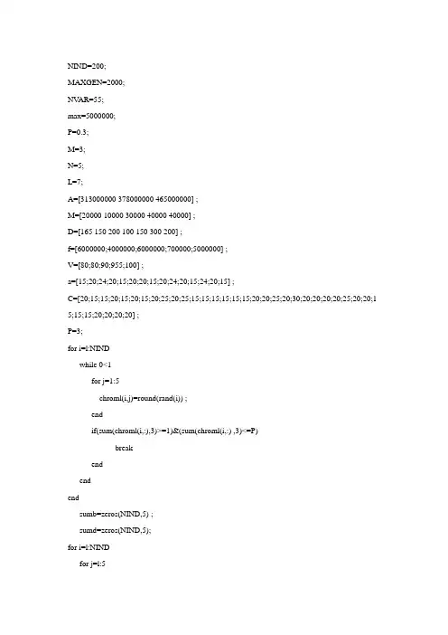
NIND=200;MAXGEN=2000;NV AR=55;max=5000000;P=0.3;M=3;N=5;L=7;A=[313000000 378000000 465000000] ;M=[20000 10000 30000 40000 40000] ;D=[165 150 200 100 150 300 200] ;f=[6000000;4000000;6000000;700000;5000000] ;V=[80;80;90;955;100] ;a=[15;20;24;20;15;20;20;15;20;24;20;15;24;20;15] ;C=[20;15;15;20;15;20;15;20;25;20;25;15;15;15;15;15;15;20;20;25;20;30;20;20;20;20;25;20;20;1 5;15;15;20;20;20;20] ;P=3;for i=l:NINDwhile 0<1for j=1:5chroml(i,j)=round(rand(i)) ;endif(sum(chroml(i,:),3)>=1)&(sum(chroml(i,:) ,3)<=P)breakendendendsumb=zeros(NIND,5) ;sumd=zeros(NIND,5);for i=l:NINDfor j=l:5if chrom1(i,j)=0chrom3(i,(2*(j-1)+1):(3*j))=0;chrom3(i, (7*(j-l)+1):(8*j))=0;elsewhile chroml(i,j)=l chrom3(i,(3*(j-1)+1):(3*j)=rand(i,3).* min(A[M(j)M(j)]);sumb(i,j)=sum(chrom3(i,(3*(j-l)+1):(3*j)),3);chrom3(j,(7*(j-1)+1):(7*j))=rand(1,7).*(rep([M(j)],[11]));sumd(i,j)=sum(chrom3(i,(7*(j-l)+1):(7*j)),3);chrom3(i,(7*(j-l)+1):(7*j))=(sumb(i,j)/sumd(i,j))*chrom3(i,(7*(j-l)+1):(7*j));if sumb(i,j)<=1.0*M(j)breakendendendendendchrom=[chroml chrorn2 chrom3];%产生初始种群[objvalue]=calobjvaluc(chrom,M,N,L,A,C, V,f);[fitvalue,restriction]=calfitvalue(objvalue,chrom,max,M,N,L,A,M,D,P); [bestindividual,bestfit,bestrestriction,nopos]=best(chrom,fitvalue,restriction);gem=0;while gen<MAXGEN,[objvalue]=calobjvalue(chrom,M,N,L,A,C,V,D);[fitvalue,restriction]=calfitvalue(objvalue,chrom,max,M,N,L,A,M,D,P); [bestindividuall,bestfitl,bestrestrictionl,noposl]=best(chrom,fitvalue,restriction);if bestrestriction>bestrestrictionlbestindividual=bestindividual l;besttit=-bestfitl;bestrestriction=bestrestriction l;endif bestrestriction =bestrcstrictionl)&(bestfit<bestfitl)bestindividual=beStindividual l;besttit=-bestfitl;bestrestriction=bestrestrictionl:endchrom(noposl,:)=bestindividual;[newchrom]=selection(chrom,fitvalue);[newchrom]=crossover(newchrom,M,N,1);[newchrom]=mutation(newchrom,P,M,N,1);[bestindividual2,bestfit2,bestrestrietion2,nopos2]=best(newchrom,fitvalue, restrietion); If bestrestriction>bestrestriction2bestindividual=bestindividual2;bestfit=bestfit2;bestrestriction=bestrestriction2;endif(bestrestriction=bestrestriction2)&(bestfit<bestfit2)bestindividual=bestindividual2;bestfit =-bestfit2;bestrestriction =bestrestriction2;endchrom=newchrom;gen=gen+1;endbestindividual,bestfit,bestrestriction%目标函数Function[objvalue]=ealobjvalue(chrom,M,N,L,A, V,f)Chrom1= chrom(:,1:N);Chrom2=chrom(:,(N+1):(N+M*N));chrom3= chrom (:,(N+M*N+1):(N+M*N+N*L));[NIND,NV AR]=size(chrom);for i=l:NINDfor j=l:Nu(i,j)=7300*sum(chrom2(i,(2*(j-l)+1):(2*j)),2);endendobjvalue=chrom2*a*7300+chrom3*c*3650+sqrt(u).* chroml*V+chroml*f; %适应度计算和约束判断Function[fitvalue restrection]=ealfitvalue(objvalue,chrom, max,M,N,l,A,M,D,P)Global gen;[NIND,NV AR]=size(chrom);Chroml=chrom (:,1:N);chrom2=Chrom(:,(N+1):(N+M*n));chrom3=Chrom(:,(N+M*N*N+1):(N+M*N+N*1));restriction=zeros(NIND,1);r=zeros(NIND,M);s=zeros(NIND,N);t=zeros(NIND,1);u=zeros(NIND,3);p=zeros(NIND,n);for i=l:NINDfor j=l:Mr(i,j)=A(j)-sum((chrom2(i,j:m:m*}n)),2);if r(i,j)<0restriction(i,1)=restriction(i,1)+1;endendfor j=l:lt(i,j)=sum((chrom3(i,j:l:n*1)),2)-D(j);if t(i,j)<0restriction(i,1)=-restriction(i,l)+1;endendfor j=l:ns(i,j)=chroml(i,j)*M(j)-sum(chrom2(i,(M*(j-1)+1):(M*j)),2);p(i,j)=abs(sum(chrom3(i,(1*(j-1)+1):(1*j)),2)-sum(chrom2(i,(M*(j-1)+1):(M*j)),2));if s(i,j)<0restrietion(i,1)=restriction(i,1)+l;endif p(i,j)>=l e-3restriction(i,1)=restriction(i,l)+l;endendu(i,1)=P-sum(chroml(i,:),2);if u(i,1)<0restriction(i,1)=restriction(i,l)+1;endu(i,2)=sum(chroml(i,:),2)-1;if u(i,2)<0restrigtion(i,1)=restriction(i,1)+l;endif(objvalue(i,1)<max)fitvaluc(i,1)=max-objvaluc(i,1);elsefitvalue(i,1)=0.0;endend%找出最优个体和最差个体function[bestindividual,bestfit,bestrestriction,nopos]=best(chrom,fitvalue,restriction); [NIND,NV AR]=size(chrom);pos=l;for i=l:NINDif restriction(pos,1)>restriction(i,1)pos=i;endif(restriction(pos,1)=restriction(i,1))&(fitvalue(pos,1)<fitvalue(i,1)) pos=i;endendbestindividual=chrom(pos,:);bestfit=fitvalue(pos);bestrestriction= restriction (pos,:);nopos=1;for i=l:NINDif restriction(nopos,1)<restriction(i,1)nopos=i;endif(restriction(nopos,1)=restriction(i,1))&(fitvalue(nopos,1)>fitvalue(i,1)) nopos=i;endend%选择Function[newchrom]=selection(chrom,fitvalue)totalfit=sum(fitvalue);fitvalue=:fitvalue/totalfit;fitvalue=cumsum(fitvalue);[NIND,NV AR]=size(chrom);ms=sort(rand(NIND,1));fitin=1;newin=1;while newin<=NINDif(ms(newin))<fitvalue(fitin)temp(newin,:)=chrom(fitin,:);newin=newin+1;elsefitin=fitin+1;endif fitin>=NINDfitin=NIND;endendnewchrom=temp;%交叉Function[newchrom]=crossover(chrom,M,N,1)global gen;[NIND,SVAR]=size(chrom);chrom1=chrom(:,l:n);chrom2=chrom(:, (N+1) : (N+M*N)) ;chrom3=chrom(:, (N+m*n+1) : (N+M*N+N*1)) ; newchrom=zeros(NIND,NV AR) ;P=0.75;for i=l:2:NIND-1if(rand<P)point=ceil(rand*(N-1));ifpoint<5newchrom(i,:)=[chroml(i,l:point)chromI(i+1,point+1:n) ... chrom2(i,l:M*point)chrom2(i+l,M*point+1:M*N) ... chrom3(i,1:l*point)chrom3(i+l,1*point+l:N*1)]; newchrom(i+l,:)=[chroml(i+l,1:point)chroml(i,point+l:n) ... chrom2(i+l,l:m*point)chrom2(i,M*point+l:M*N) ...chrom3(i+1,1:l*point)chrom3(i,1*point+l:N*1)];elsenewchrom(i,:)=chrom(i,:);newchrom(i+1,:)=chrom(i+l,:);endelsenewchrom(i,:)=chromo,:);newchrom(i+l,:)=chrom(i+l,:);endend%变异Function[newchrom]=mutation(chrom,P,M,N,L)global gen;FieldDR=[0 0 0 0 0 0 0 0 0 0 0 0 0 0 0;20000 20000 10000 10000 30000 30000 40000 40000 40000 40000];RANGE=[0 0 0 0 0 0 0;165 150 200 100 150 300 200];[NIND,NV AR]=size(chrom);chroml=chrom(:,l:N);chrom2=chrom(:, (N+1):(N+M*N));chrom3=chrom(:, (N+M*N+1):(N+M*n+ 1));newchrom=zeros(NIND,NV AR);newchroml=zeros(NIND,N);newchrom2=zeros(NIND,M*N);newchrom3=zeros(NIND,N*1);for i=1:NINDfor j=l:Nif chrom l(i,j)=0newchrom2(i,(M*(j-1)+1):(M*j))=0;newchrom3(i,1*(j-l)+1):(1*j)=0;elseif round(rand)=0newchrom2(i,(M*(j-1)+1):(M*j))=chrom2(i,(M*(j-1)+1):(M*j)+ ...(FieldDR(2,(M*(j-1)+1):(M*j))=chrom2(i,(M*(j-1)+1):(M*j)))*(1-rand^((1-gen/2000)^10));newchrom3(i,(1*(j-1)+1):(1*j)=chrom3(i,(1*(j-1)+1):(1*j) + ...([165 150 200 100 150 300 200]-chrom3(i,(1*(j-1)+1):(1*j)))*(1-rand^((1*gen/2000)^10));elseif round(rand)=lnewChrom2(i,(M*(j-1)+1):(M*j) ) = Chrom2 (i,(M*(j-1)+1):(M*j)) ...(chrom2(i,(M*(j-1)+1):(M*j))-[00])*(1-rand^((1-gen/2000)^10));newchrom3(i,(1*(j-1)+1):(1*j)):chrom3(i,(1*(j-1)+1):(1*j)) ...(chrom3(i,(1*(j-1)+1):(N))-[0 0 0 0 0 0 0 0])*(1-rand^((1*gen/2000)^10));endendendendnewchrom1=chrom1;newchrom=[newchrom1 newchrom2 newchrom3];endendnewchrom1=chrom1;newchrom=[newchrom1 newchrom2 newchrom3];bestindividualbestindividual=columms 1 through 171.0000 1.0000 0 0 1.000 80.3686 20.6636 0 0 23.7458 50.7648 63.57695 0 0 123.6753 39.7648 19.5769 0 0 289.6753 columms 18 through 3419.5849 50.7648 45.7985 64.2875 19.9768 53.6843 135.6752 32.6437 24.5342 27.9485 9.9873 24.7638 125.7958 27.8745 columms 35 through 510 0 0 0 0 0 00 0 0 0 0 0 0columms 52 through 5595.7482 35.9862 83.4768 28.4769 74.5867 113.4786 44.4873。
matlab教程ppt(完整版)
可以使用`'`运算符对矩阵进行 转置。
矩阵高级运算
01
逆矩阵
可以使用`inv`函数求矩阵的逆矩阵 。
行列式
可以使用`det`函数求矩阵的行列式 。
03
02
特征值和特征向量
可以使用`eig`函数求矩阵的特征值 和特征向量。
秩
可以使用`rank`函数求矩阵的秩。
04
04
matlab绘图功能
绘图基本命令
控制设计
MATLAB提供了控制系统设计和分析 工具箱,可以方便地进行控制系统的 建模、分析和优化。
03
信号处理
MATLAB提供了丰富的信号处理工具 箱,可以进行信号的时域和频域分析 、滤波器设计等操作。
05
04
图像处理
MATLAB提供了图像处理工具箱,可 以进行图像的增强、分割、特征提取 等操作。
02
matlab程序调试技巧分享
01
调试模式
MATLAB提供了调试模式,可以 逐行执行代码,查看变量值,设 置断点等。
日志输出
02
03
错误处理
通过使用fprintf函数,可以在程 序运行过程中输出日志信息,帮 助定位问题。
MATLAB中的错误处理机制可以 帮助我们捕获和处理运行时错误 。
matlab程序优化方法探讨
显示结果
命令执行后,结果将在命令窗口中显示。
保存结果
可以使用`save`命令将结果保存到文件中。
matlab变量定义与赋值
定义变量
使用`varname = value`格式定义变 量,其中`varname`是变量名, `value`是变量的值。
赋值操作
使用`=`运算符将值赋给变量。例如 ,`a = 10`将值10赋给变量a。
matlab教程ppt(完整版)
控制流语句
使用条件语句(如if-else)和 循环语句(如for)来控制程序 流程。
变量定义
使用赋值语句定义变量,例如 `a = 5`。
矩阵运算
使用矩阵进行数学运算,如加 法、减法、乘法和除法等。
函数编写
创建自定义函数来执行特定任 务。
02
MATLAB编程语言基础
变量与数据类型
变量命名规则
数据类型转换
编辑器是一个文本编辑器 ,用于编写和编辑 MATLAB脚本和函数。
工具箱窗口提供了一系列 用于特定任务的工具和功 能,如数据可视化、信号 处理等。
工作空间窗口显示当前工 作区中的变量,可以查看 和修改变量的值。
MATLAB基本操作
数据类型
MATLAB支持多种数据类型, 如数值型、字符型和逻辑型等 。
04
MATLAB数值计算
数值计算基础
01
02
03
数值类型
介绍MATLAB中的数值类 型,包括双精度、单精度 、复数等。
变量赋值
讲解如何给变量赋值,包 括标量、向量和矩阵。
运算符
介绍基本的算术运算符、 关系运算符和逻辑运算符 及其优先级。
数值计算函数
数学函数
列举常用的数学函数,如 三角函数、指数函数、对 数函数等。
矩阵的函数运算
总结词:MATLAB提供了许多内置函 数,可以对矩阵进行各种复杂的运算
。
详细描述
矩阵求逆:使用 `inv` 函数求矩阵的 逆。
特征值和特征向量:使用 `eig` 函数 计算矩阵的特征值和特征向量。
行列式值:使用 `det` 函数计算矩阵 的行列式值。
矩阵分解:使用 `factor` 和 `expm` 等函数对矩阵进行分解和计算指数。
MATLAB经典教程(全)PPT课件
MATLAB的优势
易于学习、使用灵活、高效的数值计 算和可视化功能、强大的工具箱支持。
发展历程
从最初的数值计算工具,逐渐发展成 为一款功能强大的科学计算软件,广 泛应用于工程、科学、经济等领域。
MATLAB工作环境与界面
MATLAB工作环境
包括命令窗口、工作空间、命令历史窗口、当 前文件夹窗口等。
界面介绍
详细讲解MATLAB界面的各个组成部分,如菜 单栏、工具栏、编辑器窗口等。
基本操作
介绍如何在MATLAB环境中创建、保存、运行脚本和函数,以及如何进行基本 的文件操作。
基本数据类型与运算
矩阵大小
使用`size`函数获取矩阵的行数 和列数。
矩阵元素访问
通过下标访问矩阵元素,如 `A(i,j)`表示访问矩阵A的第i行第j 列元素。
矩阵基本操作
包括矩阵的加、减、数乘、转置 等操作。
矩阵运算及性质
矩阵乘法 满足乘法交换律和结合律,但不满足 乘法交换律。
矩阵的逆
对于方阵,若存在一矩阵B,使得 AB=BA=I(I为单位矩阵),则称B 为A的逆矩阵。
Hale Waihona Puke 03 数据分析与可视化数据导入、导出及预处理
数据导入
介绍如何使用MATLAB导入各种格式的数据文件, 如.csv、.txt、.xlsx等。
数据导出
讲解如何将MATLAB中的数据导出为常见的数据文件格式,以 便于数据共享和交换。
数据预处理
阐述数据清洗、数据变换、数据规约等预处理技术,为后续的数 据分析和可视化奠定基础。
01
02
matlab编程实例100例(精编文档).doc
【最新整理,下载后即可编辑】1-32是:图形应用篇33-66是:界面设计篇67-84是:图形处理篇85-100是:数值分析篇实例1:三角函数曲线(1)function shili01h0=figure('toolbar','none',...'position',[198****0300],...'name','实例01');h1=axes('parent',h0,...'visible','off');x=-pi:0.05:pi;y=sin(x);plot(x,y);xlabel('自变量X');ylabel('函数值Y');title('SIN( )函数曲线');grid on实例2:三角函数曲线(2)function shili02h0=figure('toolbar','none',...'position',[200 150 450 350],...'name','实例02');x=-pi:0.05:pi;y=sin(x)+cos(x);plot(x,y,'-*r','linewidth',1);grid onxlabel('自变量X');ylabel('函数值Y');title('三角函数');实例3:图形的叠加function shili03h0=figure('toolbar','none',...'position',[200 150 450 350],...'name','实例03');x=-pi:0.05:pi;y1=sin(x);y2=cos(x);plot(x,y1,...'-*r',...x,y2,...'--og');grid onxlabel('自变量X');ylabel('函数值Y');title('三角函数');实例4:双y轴图形的绘制function shili04h0=figure('toolbar','none',...'position',[200 150 450 250],...'name','实例04');x=0:900;a=1000;b=0.005;y1=2*x;y2=cos(b*x);[haxes,hline1,hline2]=plotyy(x,y1,x,y2,'semilogy','plot'); axes(haxes(1))ylabel('semilog plot');axes(haxes(2))ylabel('linear plot');实例5:单个轴窗口显示多个图形function shili05h0=figure('toolbar','none',...'position',[200 150 450 250],...'name','实例05');t=0:pi/10:2*pi;[x,y]=meshgrid(t);subplot(2,2,1)plot(sin(t),cos(t))axis equalsubplot(2,2,2)z=sin(x)-cos(y);plot(t,z)axis([0 2*pi -2 2])subplot(2,2,3)h=sin(x)+cos(y);plot(t,h)axis([0 2*pi -2 2])subplot(2,2,4)g=(sin(x).^2)-(cos(y).^2);plot(t,g)axis([0 2*pi -1 1])实例6:图形标注function shili06h0=figure('toolbar','none',...'position',[200 150 450 400],...'name','实例06');t=0:pi/10:2*pi;h=plot(t,sin(t));xlabel('t=0到2\pi','fontsize',16);ylabel('sin(t)','fontsize',16);title('\it{从0to2\pi 的正弦曲线}','fontsize',16) x=get(h,'xdata');y=get(h,'ydata');imin=find(min(y)==y);imax=find(max(y)==y);text(x(imin),y(imin),...['\leftarrow最小值=',num2str(y(imin))],...'fontsize',16)text(x(imax),y(imax),...['\leftarrow最大值=',num2str(y(imax))],...'fontsize',16)实例7:条形图形function shili07h0=figure('toolbar','none',...'position',[200 150 450 350],...'name','实例07');tiao1=[562 548 224 545 41 445 745 512];tiao2=[47 48 57 58 54 52 65 48];t=0:7;bar(t,tiao1)xlabel('X轴');ylabel('TIAO1值');h1=gca;h2=axes('position',get(h1,'position'));plot(t,tiao2,'linewidth',3)set(h2,'yaxislocation','right','color','none','xticklabel',[]) 实例8:区域图形function shili08h0=figure('toolbar','none',...'position',[200 150 450 250],...'name','实例08');x=91:95;profits1=[88 75 84 93 77];profits2=[51 64 54 56 68];profits3=[42 54 34 25 24];profits4=[26 38 18 15 4];area(x,profits1,'facecolor',[0.5 0.9 0.6],...'edgecolor','b',...'linewidth',3)hold onarea(x,profits2,'facecolor',[0.9 0.85 0.7],...'edgecolor','y',...'linewidth',3)hold onarea(x,profits3,'facecolor',[0.3 0.6 0.7],...'edgecolor','r',...'linewidth',3)hold onarea(x,profits4,'facecolor',[0.6 0.5 0.9],...'edgecolor','m',...'linewidth',3)hold offset(gca,'xtick',[91:95])set(gca,'layer','top')gtext('\leftarrow第一季度销量') gtext('\leftarrow第二季度销量') gtext('\leftarrow第三季度销量') gtext('\leftarrow第四季度销量') xlabel('年','fontsize',16);ylabel('销售量','fontsize',16);实例9:饼图的绘制function shili09h0=figure('toolbar','none',...'position',[200 150 450 250],...'name','实例09');t=[54 21 35;68 54 35;45 25 12;48 68 45;68 54 69];x=sum(t);h=pie(x);textobjs=findobj(h,'type','text');str1=get(textobjs,{'string'});val1=get(textobjs,{'extent'});oldext=cat(1,val1{:});names={'商品一:';'商品二:';'商品三:'};str2=strcat(names,str1);set(textobjs,{'string'},str2)val2=get(textobjs,{'extent'});newext=cat(1,val2{:});offset=sign(oldext(:,1)).*(newext(:,3)-oldext(:,3))/2; pos=get(textobjs,{'position'});textpos=cat(1,pos{:});textpos(:,1)=textpos(:,1)+offset;set(textobjs,{'position'},num2cell(textpos,[3,2]))实例10:阶梯图function shili10h0=figure('toolbar','none',...'position',[200 150 450 400],...'name','实例10');a=0.01;b=0.5;t=0:10;f=exp(-a*t).*sin(b*t);stairs(t,f)hold onplot(t,f,':*')hold offglabel='函数e^{-(\alpha*t)}sin\beta*t的阶梯图'; gtext(glabel,'fontsize',16)xlabel('t=0:10','fontsize',16)axis([0 10 -1.2 1.2])实例11:枝干图function shili11h0=figure('toolbar','none',...'position',[200 150 450 350],...'name','实例11');x=0:pi/20:2*pi;y1=sin(x);y2=cos(x);h1=stem(x,y1+y2);hold onh2=plot(x,y1,'^r',x,y2,'*g');hold offh3=[h1(1);h2];legend(h3,'y1+y2','y1=sin(x)','y2=cos(x)') xlabel('自变量X');ylabel('函数值Y');title('正弦函数与余弦函数的线性组合'); 实例12:罗盘图function shili12h0=figure('toolbar','none',...'position',[200 150 450 250],...'name','实例12');winddirection=[54 24 65 84256 12 235 62125 324 34 254];windpower=[2 5 5 36 8 12 76 14 10 8];rdirection=winddirection*pi/180;[x,y]=pol2cart(rdirection,windpower); compass(x,y);desc={'风向和风力','北京气象台','10月1日0:00到','10月1日12:00'};gtext(desc)实例13:轮廓图function shili13h0=figure('toolbar','none',...'position',[200 150 450 250],...'name','实例13');[th,r]=meshgrid((0:10:360)*pi/180,0:0.05:1); [x,y]=pol2cart(th,r);z=x+i*y;f=(z.^4-1).^(0.25);contour(x,y,abs(f),20)axis equalxlabel('实部','fontsize',16);ylabel('虚部','fontsize',16);h=polar([0 2*pi],[0 1]);delete(h)hold oncontour(x,y,abs(f),20)实例14:交互式图形function shili14h0=figure('toolbar','none',...'position',[200 150 450 250],...'name','实例14');axis([0 10 0 10]);hold onx=[];y=[];n=0;disp('单击鼠标左键点取需要的点'); disp('单击鼠标右键点取最后一个点'); but=1;while but==1[xi,yi,but]=ginput(1);plot(xi,yi,'bo')n=n+1;disp('单击鼠标左键点取下一个点');x(n,1)=xi;y(n,1)=yi;endt=1:n;ts=1:0.1:n;xs=spline(t,x,ts);ys=spline(t,y,ts);plot(xs,ys,'r-');hold off实例14:交互式图形function shili14h0=figure('toolbar','none',...'position',[200 150 450 250],...'name','实例14');axis([0 10 0 10]);hold onx=[];y=[];n=0;disp('单击鼠标左键点取需要的点'); disp('单击鼠标右键点取最后一个点'); but=1;while but==1[xi,yi,but]=ginput(1);plot(xi,yi,'bo')n=n+1;disp('单击鼠标左键点取下一个点');x(n,1)=xi;y(n,1)=yi;endt=1:n;ts=1:0.1:n;xs=spline(t,x,ts);ys=spline(t,y,ts);plot(xs,ys,'r-');hold off实例15:变换的傅立叶函数曲线function shili15h0=figure('toolbar','none',...'position',[200 150 450 250],...'name','实例15');axis equalm=moviein(20,gcf);set(gca,'nextplot','replacechildren')h=uicontrol('style','slider','position',...[100 10 500 20],'min',1,'max',20)for j=1:20plot(fft(eye(j+16)))set(h,'value',j)m(:,j)=getframe(gcf);endclf;axes('position',[0 0 1 1]);movie(m,30)实例16:劳伦兹非线形方程的无序活动function shili15h0=figure('toolbar','none',...'position',[200 150 450 250],...'name','实例15');axis equalm=moviein(20,gcf);set(gca,'nextplot','replacechildren')h=uicontrol('style','slider','position',...[100 10 500 20],'min',1,'max',20)for j=1:20plot(fft(eye(j+16)))set(h,'value',j)m(:,j)=getframe(gcf);endclf;axes('position',[0 0 1 1]);movie(m,30)实例17:填充图function shili17h0=figure('toolbar','none',...'position',[200 150 450 250],...'name','实例17');t=(1:2:15)*pi/8;x=sin(t);y=cos(t);fill(x,y,'r')axis square offtext(0,0,'STOP',...'color',[1 1 1],...'fontsize',50,...'horizontalalignment','center') 例18:条形图和阶梯形图function shili18h0=figure('toolbar','none',...'position',[200 150 450 250],...'name','实例18');subplot(2,2,1)x=-3:0.2:3;y=exp(-x.*x);bar(x,y)title('2-D Bar Chart')subplot(2,2,2)x=-3:0.2:3;y=exp(-x.*x);bar3(x,y,'r')title('3-D Bar Chart')subplot(2,2,3)x=-3:0.2:3;y=exp(-x.*x);stairs(x,y)title('Stair Chart')subplot(2,2,4)x=-3:0.2:3;y=exp(-x.*x);barh(x,y)title('Horizontal Bar Chart')实例19:三维曲线图function shili19h0=figure('toolbar','none',...'position',[200 150 450 400],...'name','实例19');subplot(2,1,1)x=linspace(0,2*pi);y1=sin(x);y2=cos(x);y3=sin(x)+cos(x);z1=zeros(size(x));z2=0.5*z1;z3=z1;plot3(x,y1,z1,x,y2,z2,x,y3,z3)grid onxlabel('X轴');ylabel('Y轴');zlabel('Z轴');title('Figure1:3-D Plot')subplot(2,1,2)x=linspace(0,2*pi);y1=sin(x);y2=cos(x);y3=sin(x)+cos(x);z1=zeros(size(x));z2=0.5*z1;z3=z1;plot3(x,z1,y1,x,z2,y2,x,z3,y3)grid onxlabel('X轴');ylabel('Y轴');zlabel('Z轴');title('Figure2:3-D Plot')实例20:图形的隐藏属性function shili20h0=figure('toolbar','none',...'position',[200 150 450 300],...'name','实例20');subplot(1,2,1)[x,y,z]=sphere(10);mesh(x,y,z)axis offtitle('Figure1:Opaque')hidden onsubplot(1,2,2)[x,y,z]=sphere(10);mesh(x,y,z)axis offtitle('Figure2:Transparent') hidden off实例21PEAKS函数曲线function shili21h0=figure('toolbar','none',...'position',[200 100 450 450],...'name','实例21');[x,y,z]=peaks(30);subplot(2,1,1)x=x(1,:);y=y(:,1);i=find(y>0.8&y<1.2);j=find(x>-0.6&x<0.5);z(i,j)=nan*z(i,j);surfc(x,y,z)xlabel('X轴');ylabel('Y轴');zlabel('Z轴');title('Figure1:surfc函数形成的曲面') subplot(2,1,2)x=x(1,:);y=y(:,1);i=find(y>0.8&y<1.2);j=find(x>-0.6&x<0.5);z(i,j)=nan*z(i,j);surfl(x,y,z)xlabel('X轴');ylabel('Y轴');zlabel('Z轴');title('Figure2:surfl函数形成的曲面') 实例22:片状图function shili22h0=figure('toolbar','none',...'position',[200 150 550 350],...'name','实例22');subplot(1,2,1)x=rand(1,20);y=rand(1,20);z=peaks(x,y*pi);t=delaunay(x,y);trimesh(t,x,y,z)hidden offtitle('Figure1:Triangular Surface Plot'); subplot(1,2,2)x=rand(1,20);y=rand(1,20);z=peaks(x,y*pi);t=delaunay(x,y);trisurf(t,x,y,z)title('Figure1:Triangular Surface Plot'); 实例23:视角的调整function shili23h0=figure('toolbar','none',...'position',[200 150 450 350],...'name','实例23');x=-5:0.5:5;[x,y]=meshgrid(x);r=sqrt(x.^2+y.^2)+eps;z=sin(r)./r;subplot(2,2,1)surf(x,y,z)xlabel('X-axis')ylabel('Y-axis')zlabel('Z-axis')title('Figure1')view(-37.5,30)subplot(2,2,2)surf(x,y,z)xlabel('X-axis')ylabel('Y-axis')zlabel('Z-axis')title('Figure2')view(-37.5+90,30) subplot(2,2,3)surf(x,y,z)xlabel('X-axis')ylabel('Y-axis')zlabel('Z-axis')title('Figure3')view(-37.5,60)subplot(2,2,4)surf(x,y,z)xlabel('X-axis')ylabel('Y-axis')zlabel('Z-axis')title('Figure4')view(180,0)实例24:向量场的绘制function shili24h0=figure('toolbar','none',...'position',[200 150 450 350],...'name','实例24');subplot(2,2,1)z=peaks;ribbon(z)title('Figure1')subplot(2,2,2)[x,y,z]=peaks(15);[dx,dy]=gradient(z,0.5,0.5); contour(x,y,z,10)hold onquiver(x,y,dx,dy)hold offtitle('Figure2')subplot(2,2,3)[x,y,z]=peaks(15);[nx,ny,nz]=surfnorm(x,y,z);surf(x,y,z)hold onquiver3(x,y,z,nx,ny,nz)hold offtitle('Figure3')subplot(2,2,4)x=rand(3,5);y=rand(3,5);z=rand(3,5);c=rand(3,5);fill3(x,y,z,c)grid ontitle('Figure4')实例25:灯光定位function shili25h0=figure('toolbar','none',...'position',[200 150 450 250],...'name','实例25');vert=[1 1 1;1 2 1;2 2 1;2 1 1;1 1 2;12 2;2 2 2;2 1 2];fac=[1 2 3 4;2 6 7 3;4 3 7 8;15 8 4;1 2 6 5;5 6 7 8];grid offsphere(36)h=findobj('type','surface');set(h,'facelighting','phong',...'facecolor',...'interp',...'edgecolor',[0.4 0.4 0.4],...'backfacelighting',...'lit')hold onpatch('faces',fac,'vertices',vert,...'facecolor','y');light('position',[1 3 2]);light('position',[-3 -1 3]);material shinyaxis vis3d offhold off实例26:柱状图function shili26h0=figure('toolbar','none',...'position',[200 50 450 450],...'name','实例26'); subplot(2,1,1)x=[5 2 18 7 39 8 65 5 54 3 2];bar(x)xlabel('X轴');ylabel('Y轴');title('第一子图');subplot(2,1,2)y=[5 2 18 7 39 8 65 5 54 3 2];barh(y)xlabel('X轴');ylabel('Y轴');title('第二子图');实例27:设置照明方式function shili27h0=figure('toolbar','none',...'position',[200 150 450 350],...'name','实例27');subplot(2,2,1)sphereshading flatcamlight leftcamlight rightlighting flatcolorbaraxis offtitle('Figure1')subplot(2,2,2)sphereshading flatcamlight leftcamlight rightlighting gouraudcolorbaraxis offtitle('Figure2')subplot(2,2,3)sphereshading interpcamlight rightcamlight leftlighting phongaxis offtitle('Figure3')subplot(2,2,4)sphereshading flatcamlight leftcamlight rightlighting nonecolorbaraxis offtitle('Figure4')实例28:羽状图function shili28h0=figure('toolbar','none',...'position',[200 150 450 350],...'name','实例28');subplot(2,1,1)alpha=90:-10:0;r=ones(size(alpha));m=alpha*pi/180;n=r*10;[u,v]=pol2cart(m,n);feather(u,v)title('羽状图')axis([0 20 0 10])subplot(2,1,2)t=0:0.5:10;y=exp(-x*t);feather(y)title('复数矩阵的羽状图')实例29:立体透视(1)function shili29h0=figure('toolbar','none',...'position',[200 150 450 250],...'name','实例29');[x,y,z]=meshgrid(-2:0.1:2,...-2:0.1:2,...-2:0.1:2);v=x.*exp(-x.^2-y.^2-z.^2);grid onfor i=-2:0.5:2;h1=surf(linspace(-2,2,20),...linspace(-2,2,20),...zeros(20)+i);rotate(h1,[1 -1 1],30)dx=get(h1,'xdata');dy=get(h1,'ydata');dz=get(h1,'zdata');delete(h1)slice(x,y,z,v,[-2 2],2,-2)hold onslice(x,y,z,v,dx,dy,dz)hold offaxis tightview(-5,10)drawnowend实例30:立体透视(2)function shili30h0=figure('toolbar','none',...'position',[200 150 450 250],...'name','实例30');[x,y,z]=meshgrid(-2:0.1:2,...-2:0.1:2,...-2:0.1:2);v=x.*exp(-x.^2-y.^2-z.^2); [dx,dy,dz]=cylinder;slice(x,y,z,v,[-2 2],2,-2)for i=-2:0.2:2h=surface(dx+i,dy,dz);rotate(h,[1 0 0],90)xp=get(h,'xdata');yp=get(h,'ydata');zp=get(h,'zdata');delete(h)hold onhs=slice(x,y,z,v,xp,yp,zp);axis tightxlim([-3 3])view(-10,35)drawnowdelete(hs)hold offend实例31:表面图形function shili31h0=figure('toolbar','none',...'position',[200 150 550 250],...'name','实例31');subplot(1,2,1)x=rand(100,1)*16-8;y=rand(100,1)*16-8;r=sqrt(x.^2+y.^2)+eps;z=sin(r)./r;xlin=linspace(min(x),max(x),33); ylin=linspace(min(y),max(y),33); [X,Y]=meshgrid(xlin,ylin);Z=griddata(x,y,z,X,Y,'cubic'); mesh(X,Y,Z)axis tighthold onplot3(x,y,z,'.','Markersize',20) subplot(1,2,2)k=5;n=2^k-1;theta=pi*(-n:2:n)/n;phi=(pi/2)*(-n:2:n)'/n;X=cos(phi)*cos(theta);Y=cos(phi)*sin(theta);Z=sin(phi)*ones(size(theta)); colormap([0 0 0;1 1 1])C=hadamard(2^k);surf(X,Y,Z,C)axis square实例32:沿曲线移动的小球h0=figure('toolbar','none',...'position',[198****8468],...'name','实例32');h1=axes('parent',h0,...'position',[0.15 0.45 0.7 0.5],...'visible','on');t=0:pi/24:4*pi;y=sin(t);plot(t,y,'b')n=length(t);h=line('color',[0 0.5 0.5],...'linestyle','.',...'markersize',25,...'erasemode','xor');k1=uicontrol('parent',h0,...'style','pushbutton',...'position',[80 100 50 30],...'string','开始',...'callback',[...'i=1;',...'k=1;,',...'m=0;,',...'while 1,',...'if k==0,',...'break,',...'end,',...'if k~=0,',...'set(h,''xdata'',t(i),''ydata'',y(i)),',...'drawnow;,',...'i=i+1;,',...'if i>n,',...'m=m+1;,',...'i=1;,',...'end,',...'end,',...'end']);k2=uicontrol('parent',h0,...'style','pushbutton',...'position',[180 100 50 30],...'string','停止',...'callback',[...'k=0;,',...'set(e1,''string'',m),',...'p=get(h,''xdata'');,',...'q=get(h,''ydata'');,',...'set(e2,''string'',p);,',...'set(e3,''string'',q)']); k3=uicontrol('parent',h0,...'style','pushbutton',...'position',[280 100 50 30],...'string','关闭',...'callback','close');e1=uicontrol('parent',h0,...'style','edit',...'position',[60 30 60 20]);t1=uicontrol('parent',h0,...'style','text',...'string','循环次数',...'position',[60 50 60 20]);e2=uicontrol('parent',h0,...'style','edit',...'position',[180 30 50 20]);t2=uicontrol('parent',h0,...'style','text',...'string','终点的X坐标值',...'position',[155 50 100 20]);e3=uicontrol('parent',h0,...'style','edit',...'position',[300 30 50 20]);t3=uicontrol('parent',h0,...'style','text',...'string','终点的Y坐标值',...'position',[275 50 100 20]);实例33:曲线转换按钮h0=figure('toolbar','none',...'position',[200 150 450 250],...'name','实例33');x=0:0.5:2*pi;y=sin(x);h=plot(x,y);grid onhuidiao=[...'if i==1,',...'i=0;,',...'y=cos(x);,',...'delete(h),',...'set(hm,''string'',''正弦函数''),',...'h=plot(x,y);,',...'grid on,',...'else if i==0,',...'i=1;,',...'y=sin(x);,',...'set(hm,''string'',''余弦函数''),',...'delete(h),',...'h=plot(x,y);,',...'grid on,',...'end,',...'end'];hm=uicontrol(gcf,'style','pushbutton',...'string','余弦函数',...'callback',huidiao);i=1;set(hm,'position',[250 20 60 20]);set(gca,'position',[0.2 0.2 0.6 0.6])title('按钮的使用')hold on实例34:栅格控制按钮h0=figure('toolbar','none',...'position',[200 150 450 250],...'name','实例34');x=0:0.5:2*pi;y=sin(x);plot(x,y)huidiao1=[...'set(h_toggle2,''value'',0),',...'grid on,',...];huidiao2=[...'set(h_toggle1,''value'',0),',...'grid off,',...];h_toggle1=uicontrol(gcf,'style','togglebutton',...'string','grid on',...'value',0,...'position',[20 45 50 20],...'callback',huidiao1);h_toggle2=uicontrol(gcf,'style','togglebutton',...'string','grid off',...'value',0,...'position',[20 20 50 20],...'callback',huidiao2);set(gca,'position',[0.2 0.2 0.6 0.6])title('开关按钮的使用')实例35:编辑框的使用h0=figure('toolbar','none',...'position',[200 150 350 250],...'name','实例35');f='Please input the letter';huidiao1=[...'g=upper(f);,',...'set(h2_edit,''string'',g),',...];huidiao2=[...'g=lower(f);,',...'set(h2_edit,''string'',g),',...];h1_edit=uicontrol(gcf,'style','edit',...'position',[100 200 100 50],...'HorizontalAlignment','left',...'string','Please input the letter',...'callback','f=get(h1_edit,''string'');',...'background','w',...'max',5,...'min',1);h2_edit=uicontrol(gcf,'style','edit',...'HorizontalAlignment','left',...'position',[100 100 100 50],...'background','w',...'max',5,...'min',1);h1_button=uicontrol(gcf,'style','pushbutton',...'string','小写变大写',...'position',[100 45 100 20],...'callback',huidiao1);h2_button=uicontrol(gcf,'style','pushbutton',...'string','大写变小写',...'position',[100 20 100 20],...'callback',huidiao2);实例36:弹出式菜单h0=figure('toolbar','none',...'position',[200 150 450 250],...'name','实例36');x=0:0.5:2*pi;y=sin(x);h=plot(x,y);grid onhm=uicontrol(gcf,'style','popupmenu',...'string',...'sin(x)|cos(x)|sin(x)+cos(x)|exp(-sin(x))',...'position',[250 20 50 20]);set(hm,'value',1)huidiao=[...'v=get(hm,''value'');,',...'switch v,',...'case 1,',...'delete(h),',...'y=sin(x);,',...'h=plot(x,y);,',...'grid on,',...'case 2,',...'delete(h),',...'y=cos(x);,',...'h=plot(x,y);,',...'grid on,',...'case 3,',...'delete(h),',...'y=sin(x)+cos(x);,',...'h=plot(x,y);,',...'grid on,',...'case 4,',...'delete(h),',...'y=exp(-sin(x));,',...'h=plot(x,y);,',...'grid on,',...'end'];set(hm,'callback',huidiao)set(gca,'position',[0.2 0.2 0.6 0.6]) title('弹出式菜单的使用')实例37:滑标的使用h0=figure('toolbar','none',...'position',[200 150 450 250],...'name','实例37');[x,y]=meshgrid(-8:0.5:8);r=sqrt(x.^2+y.^2)+eps;z=sin(r)./r;h0=mesh(x,y,z);h1=axes('position',...[0.2 0.2 0.5 0.5],...'visible','off');htext=uicontrol(gcf,...'units','points',...'position',[20 30 45 15],...'string','brightness',...'style','text');hslider=uicontrol(gcf,...'units','points',...'position',[10 10 300 15],...'min',-1,...'max',1,...'style','slider',...'callback',...'brighten(get(hslider,''value''))'); 实例38:多选菜单h0=figure('toolbar','none',...'position',[200 150 450 250],...'name','实例38');[x,y]=meshgrid(-8:0.5:8);r=sqrt(x.^2+y.^2)+eps;z=sin(r)./r;h0=mesh(x,y,z);hlist=uicontrol(gcf,'style','listbox',...'string','default|spring|summer|autumn|winter',...'max',5,...'min',1,...'position',[20 20 80 100],...'callback',[...'k=get(hlist,''value'');,',...'switch k,',...'case 1,',...'colormap default,',...'case 2,',...'colormap spring,',...'case 3,',...'colormap summer,',...'case 4,',...'colormap autumn,',...'case 5,',...'colormap winter,',...'end']);实例39:菜单控制的使用h0=figure('toolbar','none',...'position',[200 150 450 250],...'name','实例39');x=0:0.5:2*pi;y=cos(x);h=plot(x,y);grid onset(gcf,'toolbar','none')hm=uimenu('label','example');huidiao1=[...'set(hm_gridon,''checked'',''on''),',...'set(hm_gridoff,''checked'',''off''),',...'grid on'];huidiao2=[...'set(hm_gridoff,''checked'',''on''),',...'set(hm_gridon,''checked'',''off''),',...'grid off'];hm_gridon=uimenu(hm,'label','grid on',...'checked','on',...'callback',huidiao1);hm_gridoff=uimenu(hm,'label','grid off',...'checked','off',...'callback',huidiao2);实例40:UIMENU菜单的应用h0=figure('toolbar','none',...'position',[200 150 450 250],...'name','实例40');h1=uimenu(gcf,'label','函数');h11=uimenu(h1,'label','轮廓图',...'callback',[...'set(h31,''checked'',''on''),',...'set(h32,''checked'',''off''),',...'[x,y,z]=peaks;,',...'contour3(x,y,z,30)']);h12=uimenu(h1,'label','高斯分布',...'callback',[...'set(h31,''checked'',''on''),',...'set(h32,''checked'',''off''),',...'mesh(peaks);,',...'axis tight']);。