计量 习题4-1答案
第四章酸碱滴定法课后习题及答案

第四章酸碱滴定法课后习题及答案第四章酸碱滴定法习题4-14.1 下列各种弱酸的p K a已在括号内注明,求它们的共轭碱的pK b;(1)HCN(9.21);(2)HCOOH(3.74);(3)苯酚(9.95);(4)苯甲酸(4.21)。
4.2 已知H3PO4的p K a=2.12,p K a=7.20,p K a=12.36。
求其共轭碱PO43-的pK b1,HPO42-的pK b2.和H2PO4-的p K b3。
4.3 已知琥珀酸(CH2COOH)2(以H2A表⽰)的p K al=4.19,p K b1=5.57。
试计算在pH4.88和5.0时H2A、HA-和A2-的分布系数δ2、δ1和δ0。
若该酸的总浓度为0.01mol·L-1,求pH=4.88时的三种形式的平衡浓度。
4.4 分别计算H2CO3(p K a1=6.38,pK a2=10.25)在pH=7.10,8.32及9.50时,H2CO3,HCO3-和CO32-的分布系数δ2` δ1和δ0。
4.5 已知HOAc的p Ka = 4.74,NH3·H2O的pKb=4.74。
计算下列各溶液的pH值:(1) 0.10 mol·L-1HOAc ;(2) 0.10 mol·L-1 NH3·H2O;(3) 0.15 mol·L-1 NH4Cl;(4) 0.15 mol·L-1 NaOAc。
4.6计算浓度为0.12 mol·L-1的下列物质⽔溶液的pH(括号内为p Ka)。
(1)苯酚(9.95);(2)丙烯酸(4.25);(3)吡啶的硝酸盐(C5H5NHNO3)(5.23)。
解:(1) 苯酚(9.95)4.7 计算浓度为0.12 mol·L-1的下列物质⽔溶液的pH(p Ka:见上题)。
(1)苯酚钠;(2)丙烯酸钠;(3)吡啶。
4.8 计算下列溶液的pH:(1)0.1mol·L-1NaH2PO4;(2)0.05 mol·L-1K2HPO4。
计量经济学 第二版 课后习题1-14章 中文版答案汇总
即 是条件无偏。
10.
其中 = =
= = =0
= + -2
= + -2n 2= -
= =
用n1表示n个样本中X=0的样本个数,n2表示X=1的样本个数,n1+n2=n,则:
,
= , = =
=n2
已知
= -( ) =
+ =
11.
(1) = =485.10-523.10=-38
SE( )=SE( )= = ≈7.65
2.46> = = =2.143>1.96
= = =1.038<1.96
College、Female、Age对AHE的回归系数都在1%水平下统计显著,Northeast、
Midwest对AHE的回归系数在5%水平下统计显著。South对AHE的回归系数
与$10/h差距很远。
②β1的95%置信区间为[ -1.96SE( ), +1.96SE( )],其中 =1.47,SE( )=0.07
1.3328≤β1≤1.6072
5.53312≤4β1≤6.4288
即多接受4年大学教育,平均每小时多赚[5.53312,6.4288]美元,在95%的置信水平
下与回归结果吻合。
(2) $15.67
$17.12
4.
(1)地区间平均收入存在重大差异。东北部工人平均每小时比西部工人多挣$0.69;中西部
则比西部多$0.60/h;但南部比西部少$0.27/h。
(2)因为美国将国家经济分成东北部、中西部、南部以及西部四个片区,如果不居住在东北
部、中西部、南部,那一定居住在西部,所以无需West变量即可涵盖所有的样本。
(完整版)《建筑工程计量与计价》综合练习题及答案

《建筑工程计量与计价》综合练习一一.填空题(共 20 分,每空格 1 分)1.定额按生产要素分为、、。
2 .工人在工作班内消耗的工作时间按其消耗的性质可以分为两大类:和。
3.利用坡屋顶内空间时净高超过的部位应计算全面积;净高在的部位应计算 1/2 面积;净高的部位不应计算面积。
4.构造柱混凝土与砖墙咬接深度一般为 60mm,故马牙槎宽度按一边统长计算。
5.卷材屋面其工程量按图示尺寸的乘以规定的以平方米计算。
6.独立柱一般抹灰按乘以以平方米计算。
7.工程量清单由工程量清单、清单、清单组成。
8.建筑安装工程间接费由、组成。
9.工程量清单计价,按照中华人民共和国建设部令 107 号《建筑工程施工发包与承包计价管理方法》的规定,有和两种方法。
二.选择题(共 10 分,每小题 1 分)1.某建筑物 6 层,外围水平面积 500m2 内有采光天棚(与屋面等标高)大厅 60m2 ,外有附墙通顶垃圾道 5m2 ,则该建筑物建筑面积为( )m2。
A. 3030 B. 3000 C. 2940 D. 27302.外墙墙身当有屋架且室内外有天棚者,其高度算至屋架下弦底面另加 ( )mm。
A. 300 B. 350 C. 200 D. 2503.我国采用工料单价法时,其单价是按 ( )确定的。
A.现行预算定额的工、料、机消耗标准及市场价格确定B.现行预算定额的工、料、机消耗标准及预算价格确定C.企业定额的工、料、机消耗标准及市场价格确定D.企业定额的工、料、机消耗标准及预算价格确定4.下列费用项目中不属于措施项目清单中通用项目的是 ( )。
A.安全施工 B.夜间施工 C.便道 D.已完工程及设备保护5.在工程量清单计价中,钢筋混凝土模板工程应在 ( )中列项考虑。
A.分部分项工程量清单 B.综合单价C.措施项目清单 D.其他项目清单=S+2×L+16 公式中 S 为( )。
6 .在平整场地的工程量计算中, S平A.底层占地面积 B.底层建筑面积 C.底层净面积 D.底层结构面积7.天棚吊顶面层工程量以面积计算,应扣除 ( )。
计量经济学精要第四版课后习题答案

不能,因为两个模型中的解释变量不同
f.如何判定哪一个模型更好?
除非知道X,Y分别代表什么,否则无法判断。
0.000000
1
2
3
4
B解释个回归结果
解:1. 斜率说明X每变动一个单位,Y的绝对变动量;
2. 斜率便是弹性系数;
3. 斜率表示X每变动一个单位,Y的均值的瞬时增长率;
4,. 斜率表示X的相对变化对Y的绝对量的影响。
C对每一个模型求Y对X的变化率
解:1. ; 2. ;
3. ; 4. .
D对每一个模型求Y对X的弹性,对其中的一些模型,求Y对X的均值弹性。
5.14
(1) Y对X,即
Dependent Variable: Y
Method: Least Squares
Date: 11/13/17 Time: 20:58
Sample: 1971 1987
Included observations: 17
Variable
Coefficient
Std. Error
19.72216
S.E. of regression
4.891751
Akaike info criterion
6.123109
Sum squared resid
358.9385
Schwarz criterion
6.221134
Log likelihood
-50.04642
Hannan-Quinn criter.
Sample: 1971 1987
Included observations: 17
Variable
Coefficient
工程计量与计价复习题+答案

复习题1及答案一、名词解释1.竣工清理答案:竣工清理,系指建筑物(构筑物)内、外围四周2m范围内建筑垃圾的清理、场内运输和场内指定地点的集中堆放,建筑物(构筑物)竣工验收前的清理、清洁等工作内容。
按设计图示尺寸,以建筑物(构筑物)结构外围内包的空间体积计算。
2.强夯的夯击击数答案:系指强夯机械就位后,夯锤在同一夯点上下起落的次数。
3.施工图预算答案:是由设计单位在施工图设计完成后,根据施工图设计图纸及相关资料编制的,用于确定工程预算造价及工料的工程造价的文件。
4. 运杂费答案:是指材料、工程设备自来源地运至工地仓库或指定堆放地点所发生的全部费用。
5.现场签证答案:发包人现场代表与承包人现场代表就施工过程中涉及的责任事件所作的签认证明。
6.预付款答案:用于承包人为合同工程施工购置材料、工程设备,购置或租赁施工设备、修建临时设施以及组织施工队伍进场等所需的款项。
二、单项选择题(在每小题的四个备选答案中,选出一个正确答案,并将正确答案的号码填在题中的括号内。
1、层高2.2米的仓库应按()计算建筑面积。
A、建筑物外墙勒脚以上的外围面积的1/4B、建筑物外墙勒脚以上的外围面积的1/2C、按建筑物外墙勒脚以上的外围面积D、不应2、砖外墙应以外墙( )为计算长度。
A.外边线B.中心线C.内边线D.净长线3、外墙墙身高度,对于坡屋面且室内外均有天棚者,算到屋架下弦另加()mm。
A、100B、200C、300D、2504、材料消耗定额中用以表示周转材料的消耗量是指该周转材料的()。
A、一次使用量B、回收量C、周转使用量D、摊销量5、初步设计方案通过后,在此基础上进行施工图设计,并编制()。
A、初步设计概算B、修正概算C、施工预算D、施工图预算6、整体楼梯的工程量分层按水平投影面积以平方米计算。
不扣除宽度小于()的楼梯井空隙。
A、20cmB、50cmC、70cmD、90cm7、由建设单位采购供应的材料,施工单位按采购保管费的()收取保管费。
计量经济学题库及答案
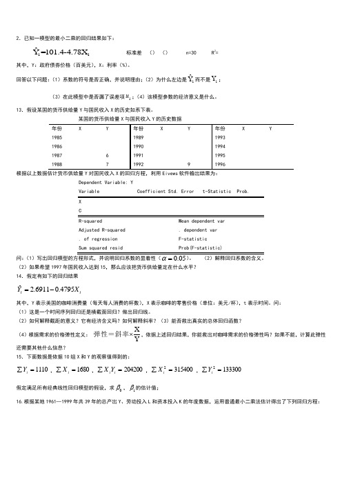
2.已知一模型的最小二乘的回归结果如下:i iˆY =101.4-4.78X 标准差 () () n=30 R 2=其中,Y :政府债券价格(百美元),X :利率(%)。
回答以下问题:(1)系数的符号是否正确,并说明理由;(2)为什么左边是iˆY 而不是i Y ; (3)在此模型中是否漏了误差项i u ;(4)该模型参数的经济意义是什么。
13.假设某国的货币供给量Y 与国民收入X 的历史如系下表。
某国的货币供给量X 与国民收入Y 的历史数据根据以上数据估计货币供给量Y 对国民收入X 的回归方程,利用Eivews 软件输出结果为:Dependent Variable: Y Variable Coefficient Std. Error t-Statistic Prob. X CR-squaredMean dependent var Adjusted R-squared . dependent var . of regression F-statistic Sum squared residProb(F-statistic)问:(1)写出回归模型的方程形式,并说明回归系数的显着性()。
(2)解释回归系数的含义。
(2)如果希望1997年国民收入达到15,那么应该把货币供给量定在什么水平?14.假定有如下的回归结果tt X Y 4795.06911.2ˆ-= 其中,Y 表示美国的咖啡消费量(每天每人消费的杯数),X 表示咖啡的零售价格(单位:美元/杯),t 表示时间。
问: (1)这是一个时间序列回归还是横截面回归?做出回归线。
(2)如何解释截距的意义?它有经济含义吗?如何解释斜率?(3)能否救出真实的总体回归函数? (4)根据需求的价格弹性定义: YX⨯弹性=斜率,依据上述回归结果,你能救出对咖啡需求的价格弹性吗?如果不能,计算此弹性还需要其他什么信息?15.下面数据是依据10组X 和Y 的观察值得到的:1110=∑i Y ,1680=∑iX ,204200=∑ii Y X ,3154002=∑i X ,1333002=∑iY假定满足所有经典线性回归模型的假设,求0β,1β的估计值;16.根据某地1961—1999年共39年的总产出Y 、劳动投入L 和资本投入K 的年度数据,运用普通最小二乘法估计得出了下列回归方程:,DW=式下括号中的数字为相应估计量的标准误。
计量经济学第四版习题及参考答案
计量经济学第四版习题及参考答案The final revision was on November 23, 2020计量经济学(第四版)习题参考答案潘省初第一章 绪论试列出计量经济分析的主要步骤。
一般说来,计量经济分析按照以下步骤进行:(1)陈述理论(或假说) (2)建立计量经济模型 (3)收集数据 (4)估计参数 (5)假设检验 (6)预测和政策分析 计量经济模型中为何要包括扰动项为了使模型更现实,我们有必要在模型中引进扰动项u 来代表所有影响因变量的其它因素,这些因素包括相对而言不重要因而未被引入模型的变量,以及纯粹的随机因素。
什么是时间序列和横截面数据 试举例说明二者的区别。
时间序列数据是按时间周期(即按固定的时间间隔)收集的数据,如年度或季度的国民生产总值、就业、货币供给、财政赤字或某人一生中每年的收入都是时间序列的例子。
横截面数据是在同一时点收集的不同个体(如个人、公司、国家等)的数据。
如人口普查数据、世界各国2000年国民生产总值、全班学生计量经济学成绩等都是横截面数据的例子。
估计量和估计值有何区别估计量是指一个公式或方法,它告诉人们怎样用手中样本所提供的信息去估计总体参数。
在一项应用中,依据估计量算出的一个具体的数值,称为估计值。
如Y 就是一个估计量,1nii YY n==∑。
现有一样本,共4个数,100,104,96,130,则根据这个样本的数据运用均值估计量得出的均值估计值为5.107413096104100=+++。
第二章 计量经济分析的统计学基础略,参考教材。
请用例中的数据求北京男生平均身高的99%置信区间NSS x ==45= 用=,N-1=15个自由度查表得005.0t =,故99%置信限为 x S t X 005.0± =174±×=174±也就是说,根据样本,我们有99%的把握说,北京男高中生的平均身高在至厘米之间。
25个雇员的随机样本的平均周薪为130元,试问此样本是否取自一个均值为120元、标准差为10元的正态总体 原假设 120:0=μH备择假设 120:1≠μH 检验统计量查表96.1025.0=Z 因为Z= 5 >96.1025.0=Z ,故拒绝原假设, 即 此样本不是取自一个均值为120元、标准差为10元的正态总体。
计量经济学导论ch04习题答案
28CHAPTER 4TEACHING NOTESAt the start of this chapter is good time to remind students that a specific error distribution played no role in the results of Chapter 3. That is because only the first two moments were derived under the full set of Gauss-Markov assumptions. Nevertheless, normality is needed to obtain exact normal sampling distributions (conditional on the explanatory variables). Iemphasize that the full set of CLM assumptions are used in this chapter, but that in Chapter 5 we relax the normality assumption and still perform approximately valid inference. One could argue that the classical linear model results could be skipped entirely, and that only large-sample analysis is needed. But, from a practical perspective, students still need to know where the t distribution comes from because virtually all regression packages report t statistics and obtain p -values off of the t distribution. I then find it very easy to cover Chapter 5 quickly, by just saying we can drop normality and still use t statistics and the associated p -values as beingapproximately valid. Besides, occasionally students will have to analyze smaller data sets, especially if they do their own small surveys for a term project.It is crucial to emphasize that we test hypotheses about unknown population parameters. I tellmy students that they will be punished if they write something like H 0:1ˆβ = 0 on an exam or, even worse, H 0: .632 = 0.One useful feature of Chapter 4 is its illustration of how to rewrite a population model so that it contains the parameter of interest in testing a single restriction. I find this is easier, both theoretically and practically, than computing variances that can, in some cases, depend onnumerous covariance terms. The example of testing equality of the return to two- and four-year colleges illustrates the basic method, and shows that the respecified model can have a useful interpretation. Of course, some statistical packages now provide a standard error for linear combinations of estimates with a simple command, and that should be taught, too.One can use an F test for single linear restrictions on multiple parameters, but this is less transparent than a t test and does not immediately produce the standard error needed for aconfidence interval or for testing a one-sided alternative. The trick of rewriting the population model is useful in several instances, including obtaining confidence intervals for predictions in Chapter 6, as well as for obtaining confidence intervals for marginal effects in models with interactions (also in Chapter 6).The major league baseball player salary example illustrates the difference between individual and joint significance when explanatory variables (rbisyr and hrunsyr in this case) are highly correlated. I tend to emphasize the R -squared form of the F statistic because, in practice, it is applicable a large percentage of the time, and it is much more readily computed. I do regret that this example is biased toward students in countries where baseball is played. Still, it is one of the better examples of multicollinearity that I have come across, and students of all backgrounds seem to get the point.29SOLUTIONS TO PROBLEMS4.1 (i) H 0:3β = 0. H 1:3β > 0.(ii) The proportionate effect on n salaryis .00024(50) = .012. To obtain the percentage effect, we multiply this by 100: 1.2%. Therefore, a 50 point ceteris paribus increase in ros is predicted to increase salary by only 1.2%. Practically speaking, this is a very small effect for such a large change in ros .(iii) The 10% critical value for a one-tailed test, using df = ∞, is obtained from Table G.2 as 1.282. The t statistic on ros is .00024/.00054 ≈ .44, which is well below the critical value. Therefore, we fail to reject H 0 at the 10% significance level.(iv) Based on this sample, the estimated ros coefficient appears to be different from zero only because of sampling variation. On the other hand, including ros may not be causing any harm; it depends on how correlated it is with the other independent variables (although these are very significant even with ros in the equation).4.2 (i) and (iii) generally cause the t statistics not to have a t distribution under H 0.Homoskedasticity is one of the CLM assumptions. An important omitted variable violates Assumption MLR.3. The CLM assumptions contain no mention of the sample correlations among independent variables, except to rule out the case where the correlation is one.4.3 (i) While the standard error on hrsemp has not changed, the magnitude of the coefficient has increased by half. The t statistic on hrsemp has gone from about –1.47 to –2.21, so now the coefficient is statistically less than zero at the 5% level. (From Table G.2 the 5% critical value with 40 df is –1.684. The 1% critical value is –2.423, so the p -value is between .01 and .05.)(ii) If we add and subtract 2βlog(employ ) from the right-hand-side and collect terms, we havelog(scrap ) = 0β + 1βhrsemp + [2βlog(sales) – 2βlog(employ )] + [2βlog(employ ) + 3βlog(employ )] + u = 0β + 1βhrsemp + 2βlog(sales /employ ) + (2β + 3β)log(employ ) + u ,where the second equality follows from the fact that log(sales /employ ) = log(sales ) – log(employ ). Defining 3θ ≡ 2β + 3β gives the result.30(iii) No. We are interested in the coefficient on log(employ ), which has a t statistic of .2, which is very small. Therefore, we conclude that the size of the firm, as measured by employees, does not matter, once we control for training and sales per employee (in a logarithmic functional form).(iv) The null hypothesis in the model from part (ii) is H 0:2β = –1. The t statistic is [–.951 – (–1)]/.37 = (1 – .951)/.37 ≈ .132; this is very small, and we fail to reject whether we specify a one- or two-sided alternative.4.4 (i) In columns (2) and (3), the coefficient on profmarg is actually negative, although its t statistic is only about –1. It appears that, once firm sales and market value have been controlled for, profit margin has no effect on CEO salary.(ii) We use column (3), which controls for the most factors affecting salary. The t statistic on log(mktval ) is about 2.05, which is just significant at the 5% level against a two-sided alternative. (We can use the standard normal critical value, 1.96.) So log(mktval ) is statistically significant. Because the coefficient is an elasticity, a ceteris paribus 10% increase in market value is predicted to increase salary by 1%. This is not a huge effect, but it is not negligible, either.(iii) These variables are individually significant at low significance levels, with t ceoten ≈ 3.11 and t comten ≈ –2.79. Other factors fixed, another year as CEO with the company increases salary by about 1.71%. On the other hand, another year with the company, but not as CEO, lowers salary by about .92%. This second finding at first seems surprising, but could be related to the “superstar” effect: firms that hire CEOs from outside the company often go after a small pool of highly regarded candidates, and salaries of these people are bid up. More non-CEO years with a company makes it less likely the person was hired as an outside superstar.4.5 (i) With df = n – 2 = 86, we obtain the 5% critical value from Table G.2 with df = 90.Because each test is two-tailed, the critical value is 1.987. The t statistic for H 0:0β = 0 is about -.89, which is much less than 1.987 in absolute value. Therefore, we fail to reject 0β = 0. The t statistic for H 0: 1β = 1 is (.976 – 1)/.049 ≈ -.49, which is even less significant. (Remember, we reject H 0 in favor of H 1 in this case only if |t | > 1.987.)(ii) We use the SSR form of the F statistic. We are testing q = 2 restrictions and the df in the unrestricted model is 86. We are given SSR r = 209,448.99 and SSR ur = 165,644.51. Therefore,(209,448.99165,644.51)8611.37,165,644.512F −⎛⎞=⋅≈⎜⎟⎝⎠which is a strong rejection of H 0: from Table G.3c, the 1% critical value with 2 and 90 df is 4.85.31(iii) We use the R -squared form of the F statistic. We are testing q = 3 restrictions and there are 88 – 5 = 83 df in the unrestricted model. The F statistic is [(.829 – .820)/(1 – .829)](83/3) ≈ 1.46. The 10% critical value (again using 90 denominator df in Table G.3a) is 2.15, so we fail to reject H 0 at even the 10% level. In fact, the p -value is about .23.(iv) If heteroskedasticity were present, Assumption MLR.5 would be violated, and the F statistic would not have an F distribution under the null hypothesis. Therefore, comparing the F statistic against the usual critical values, or obtaining the p -value from the F distribution, would not be especially meaningful.4.6 (i) We need to compute the F statistic for the overall significance of the regression with n = 142 and k = 4: F = [.0395/(1 – .0395)](137/4) ≈ 1.41. The 5% critical value with 4 numerator df and using 120 for the numerator df , is 2.45, which is well above the value of F . Therefore, we fail to reject H 0: 1β = 2β = 3β = 4β = 0 at the 10% level. No explanatory variable isindividually significant at the 5% level. The largest absolute t statistic is on dkr , t dkr ≈ 1.60, which is not significant at the 5% level against a two-sided alternative.(ii) The F statistic (with the same df ) is now [.0330/(1 – .0330)](137/4) ≈ 1.17, which is even lower than in part (i). None of the t statistics is significant at a reasonable level.(iii) We probably should not use the logs, as the logarithm is not defined for firms that have zero for dkr or eps . Therefore, we would lose some firms in the regression.(iv) It seems very weak. There are no significant t statistics at the 5% level (against a two-sided alternative), and the F statistics are insignificant in both cases. Plus, less than 4% of the variation in return is explained by the independent variables.4.7 (i) .412 ± 1.96(.094), or about .228 to .596.(ii) No, because the value .4 is well inside the 95% CI.(iii) Yes, because 1 is well outside the 95% CI.4.8 (i) With df = 706 – 4 = 702, we use the standard normal critical value (df = ∞ in Table G.2), which is 1.96 for a two-tailed test at the 5% level. Now t educ = −11.13/5.88 ≈ −1.89, so |t educ | = 1.89 < 1.96, and we fail to reject H 0: educ β = 0 at the 5% level. Also, t age ≈ 1.52, so age is also statistically insignificant at the 5% level.(ii) We need to compute the R -squared form of the F statistic for joint significance. But F = [(.113 − .103)/(1 − .113)](702/2) ≈ 3.96. The 5% critical value in the F 2,702 distribution can be obtained from Table G.3b with denominator df = ∞: cv = 3.00. Therefore, educ and age are jointly significant at the 5% level (3.96 > 3.00). In fact, the p -value is about .019, and so educ and age are jointly significant at the 2% level.32(iii) Not really. These variables are jointly significant, but including them only changes the coefficient on totwrk from –.151 to –.148.(iv) The standard t and F statistics that we used assume homoskedasticity, in addition to the other CLM assumptions. If there is heteroskedasticity in the equation, the tests are no longer valid.4.9 (i) H 0:3β = 0. H 1:3β ≠ 0.(ii) Other things equal, a larger population increases the demand for rental housing, which should increase rents. The demand for overall housing is higher when average income is higher, pushing up the cost of housing, including rental rates.(iii) The coefficient on log(pop ) is an elasticity. A correct statement is that “a 10% increase in population increases rent by .066(10) = .66%.”(iv) With df = 64 – 4 = 60, the 1% critical value for a two-tailed test is 2.660. The t statistic is about 3.29, which is well above the critical value. So 3β is statistically different from zero at the 1% level.4.10 (i) We use Property VAR.3 from Appendix B: Var(1ˆβ − 32ˆβ) = Var (1ˆβ) + 9 Var (2ˆβ) – 6 Cov (1ˆβ,2ˆβ).(ii) t = (1ˆβ− 32ˆβ − 1)/se(1ˆβ− 32ˆβ), so we need the standard error of 1ˆβ − 32ˆβ.(iii) Because1θ = 1β – 3β2, we can write 1β = 1θ + 3β2. Plugging this into the population model gives y = 0β + (1θ + 3β2)x 1 + 2βx 2 + 3βx 3 + u = 0β + 1θx 1 + 2β(3x 1 + x 2) + 3βx 3 + u .This last equation is what we would estimate by regressing y on x 1, 3x 1 + x 2, and x 3. The coefficient and standard error on x 1 are what we want.4.11 (i) Holding profmarg fixed, n rdintensΔ = .321 Δlog(sales ) = (.321/100)[100log()sales ⋅Δ] ≈ .00321(%Δsales ). Therefore, if %Δsales = 10, n rdintens Δ ≈ .032, or only about 3/100 of a percentage point. For such a large percentage increase in sales,this seems like a practically small effect.33(ii) H 0:1β = 0 versus H 1:1β > 0, where 1β is the population slope on log(sales ). The t statistic is .321/.216 ≈ 1.486. The 5% critical value for a one-tailed test, with df = 32 – 3 = 29, is obtained from Table G.2 as 1.699; so we cannot reject H 0 at the 5% level. But the 10% critical value is 1.311; since the t statistic is above this value, we reject H 0 in favor of H 1 at the 10% level.(iii) Not really. Its t statistic is only 1.087, which is well below even the 10% critical value for a one-tailed test.34SOLUTIONS TO COMPUTER EXERCISESC4.1 (i) Holding other factors fixed,111log()(/100)[100log()](/100)(%),voteA expendA expendA expendA βββΔ=Δ=⋅Δ≈Δwhere we use the fact that 100log()expendA ⋅Δ ≈ %expendA Δ. So 1β/100 is the (ceteris paribus) percentage point change in voteA when expendA increases by one percent.(ii) The null hypothesis is H 0: 2β = –1β, which means a z% increase in expenditure by A and a z% increase in expenditure by B leaves voteA unchanged. We can equivalently write H 0: 1β + 2β = 0.(iii) The estimated equation (with standard errors in parentheses below estimates) isn voteA = 45.08 + 6.083 log(expendA ) – 6.615 log(expendB ) + .152 prtystrA (3.93) (0.382) (0.379) (.062)n = 173, R 2 = .793.The coefficient on log(expendA ) is very significant (t statistic ≈ 15.92), as is the coefficient on log(expendB ) (t statistic ≈ –17.45). The estimates imply that a 10% ceteris paribus increase in spending by candidate A increases the predicted share of the vote going to A by about .61percentage points. [Recall that, holding other factors fixed, n voteAΔ≈(6.083/100)%ΔexpendA ).] Similarly, a 10% ceteris paribus increase in spending by B reduces n voteAby about .66 percentage points. These effects certainly cannot be ignored.While the coefficients on log(expendA ) and log(expendB ) are of similar magnitudes (andopposite in sign, as we expect), we do not have the standard error of 1ˆβ + 2ˆβ, which is what we would need to test the hypothesis from part (ii).(iv) Write1θ = 1β +2β, or 1β = 1θ– 2β. Plugging this into the original equation, and rearranging, givesn voteA = 0β + 1θlog(expendA ) + 2β[log(expendB ) – log(expendA )] +3βprtystrA + u ,When we estimate this equation we obtain 1θ≈ –.532 and se( 1θ)≈ .533. The t statistic for the hypothesis in part (ii) is –.532/.533 ≈ –1. Therefore, we fail to reject H 0: 2β = –1β.35C4.2 (i) In the modellog(salary ) = 0β+1βLSAT +2βGPA + 3βlog(libvol ) +4βlog(cost)+5βrank + u ,the hypothesis that rank has no effect on log(salary ) is H 0:5β = 0. The estimated equation (now with standard errors) isn log()salary = 8.34 + .0047 LSAT + .248 GPA + .095 log(libvol )(0.53) (.0040) (.090) (.033)+ .038 log(cost ) – .0033 rank (.032) (.0003)n = 136, R 2 = .842.The t statistic on rank is –11, which is very significant. If rank decreases by 10 (which is a move up for a law school), median starting salary is predicted to increase by about 3.3%.(ii) LSAT is not statistically significant (t statistic ≈ 1.18) but GPA is very significance (t statistic ≈ 2.76). The test for joint significance is moot given that GPA is so significant, but for completeness the F statistic is about 9.95 (with 2 and 130 df ) and p -value ≈ .0001.(iii) When we add clsize and faculty to the regression we lose five observations. The test of their joint significant (with 2 and 131 – 8 = 123 df ) gives F ≈ .95 and p -value ≈ .39. So these two variables are not jointly significant unless we use a very large significance level.(iv) If we want to just determine the effect of numerical ranking on starting law school salaries, we should control for other factors that affect salaries and rankings. The idea is that there is some randomness in rankings, or the rankings might depend partly on frivolous factors that do not affect quality of the students. LSAT scores and GPA are perhaps good controls for student quality. However, if there are differences in gender and racial composition acrossschools, and systematic gender and race differences in salaries, we could also control for these. However, it is unclear why these would be correlated with rank . Faculty quality, as perhaps measured by publication records, could be included. Such things do enter rankings of law schools.C4.3 (i) The estimated model isn log()price = 11.67 + .000379 sqrft + .0289 bdrms (0.10) (.000043) (.0296)n = 88, R 2 = .588.36Therefore, 1ˆθ= 150(.000379) + .0289 = .0858, which means that an additional 150 square foot bedroom increases the predicted price by about 8.6%.(ii)2β= 1θ – 1501β, and solog(price ) = 0β+ 1βsqrft + (1θ – 1501β)bdrms + u=0β+ 1β(sqrft – 150 bdrms ) + 1θbdrms + u .(iii) From part (ii), we run the regressionlog(price ) on (sqrft – 150 bdrms ), bdrms ,and obtain the standard error on bdrms . We already know that 1ˆθ= .0858; now we also getse(1ˆθ) = .0268. The 95% confidence interval reported by my software package is .0326 to .1390(or about 3.3% to 13.9%).C4.4 The R -squared from the regression bwght on cigs , parity , and faminc , using all 1,388observations, is about .0348. This means that, if we mistakenly use this in place of .0364, which is the R -squared using the same 1,191 observations available in the unrestricted regression, we would obtain F = [(.0387 − .0348)/(1 − .0387)](1,185/2) ≈ 2.40, which yields p -value ≈ .091 in an F distribution with 2 and 1,1185 df . This is significant at the 10% level, but it is incorrect. The correct F statistic was computed as 1.42 in Example 4.9, with p -value ≈ .242.C4.5 (i) If we drop rbisyr the estimated equation becomesn log()salary = 11.02 + .0677 years + .0158 gamesyr (0.27) (.0121) (.0016) + .0014 bavg + .0359 hrunsyr (.0011) (.0072)n = 353, R 2= .625.Now hrunsyr is very statistically significant (t statistic ≈ 4.99), and its coefficient has increased by about two and one-half times.(ii) The equation with runsyr , fldperc , and sbasesyr added is37n log()salary = 10.41 + .0700 years + .0079 gamesyr(2.00) (.0120) (.0027)+ .00053 bavg + .0232 hrunsyr(.00110) (.0086)+ .0174 runsyr + .0010 fldperc – .0064 sbasesyr (.0051) (.0020) (.0052) n = 353, R 2 = .639.Of the three additional independent variables, only runsyr is statistically significant (t statistic = .0174/.0051 ≈ 3.41). The estimate implies that one more run per year, other factors fixed,increases predicted salary by about 1.74%, a substantial increase. The stolen bases variable even has the “wrong” sign with a t statistic of about –1.23, while fldperc has a t statistic of only .5. Most major league baseball players are pretty good fielders; in fact, the smallest fldperc is 800 (which means .800). With relatively little variation in fldperc , it is perhaps not surprising that its effect is hard to estimate.(iii) From their t statistics, bavg , fldperc , and sbasesyr are individually insignificant. The F statistic for their joint significance (with 3 and 345 df ) is about .69 with p -value ≈ .56. Therefore, these variables are jointly very insignificant.C4.6 (i) In the modellog(wage ) = 0β + 1βeduc + 2βexper + 3βtenure + uthe null hypothesis of interest is H 0: 2β = 3β.(ii) Let2θ = 2β – 3β. Then we can estimate the equationlog(wage ) = 0β + 1βeduc + 2θexper + 3β(exper + tenure ) + uto obtain the 95% CI for 2θ. This turns out to be about .0020 ± 1.96(.0047), or about -.0072 to .0112. Because zero is in this CI, 2θ is not statistically different from zero at the 5% level, and we fail to reject H 0: 2β = 3β at the 5% level.C4.7 (i) The minimum value is 0, the maximum is 99, and the average is about 56.16. (ii) When phsrank is added to (4.26), we get the following:n log() wage = 1.459 − .0093 jc + .0755 totcoll + .0049 exper + .00030 phsrank (0.024) (.0070) (.0026) (.0002) (.00024)38 n = 6,763, R 2 = .223So phsrank has a t statistic equal to only 1.25; it is not statistically significant. If we increase phsrank by 10, log(wage ) is predicted to increase by (.0003)10 = .003. This implies a .3% increase in wage , which seems a modest increase given a 10 percentage point increase in phsrank . (However, the sample standard deviation of phsrank is about 24.)(iii) Adding phsrank makes the t statistic on jc even smaller in absolute value, about 1.33, but the coefficient magnitude is similar to (4.26). Therefore, the base point remains unchanged: the return to a junior college is estimated to be somewhat smaller, but the difference is not significant and standard significant levels.(iv) The variable id is just a worker identification number, which should be randomly assigned (at least roughly). Therefore, id should not be correlated with any variable in the regression equation. It should be insignificant when added to (4.17) or (4.26). In fact, its t statistic is about .54.C4.8 (i) There are 2,017 single people in the sample of 9,275.(ii) The estimated equation isn nettfa = −43.04 + .799 inc + .843 age ( 4.08) (.060) (.092)n = 2,017, R 2 = .119.The coefficient on inc indicates that one more dollar in income (holding age fixed) is reflected in about 80 more cents in predicted nettfa ; no surprise there. The coefficient on age means that, holding income fixed, if a person gets another year older, his/her nettfa is predicted to increase by about $843. (Remember, nettfa is in thousands of dollars.) Again, this is not surprising.(iii) The intercept is not very interesting as it gives the predicted nettfa for inc = 0 and age = 0. Clearly, there is no one with even close to these values in the relevant population.(iv) The t statistic is (.843 − 1)/.092 ≈ −1.71. Against the one-sided alternative H 1: β2 < 1, the p-value is about .044. Therefore, we can reject H 0: β2 = 1 at the 5% significance level (against the one-sided alternative).(v) The slope coefficient on inc in the simple regression is about .821, which is not very different from the .799 obtained in part (ii). As it turns out, the correlation between inc and age in the sample of single people is only about .039, which helps explain why the simple and multiple regression estimates are not very different; refer back to page 84 of the text.39C4.9 (i) The results from the OLS regression, with standard errors in parentheses, aren log() psoda =−1.46 + .073 prpblck + .137 log(income ) + .380 prppov (0.29) (.031) (.027) (.133)n = 401, R 2 = .087The p -value for testing H 0: 10β= against the two-sided alternative is about .018, so that wereject H 0 at the 5% level but not at the 1% level.(ii) The correlation is about −.84, indicating a strong degree of multicollinearity. Yet eachcoefficient is very statistically significant: the t statistic for log()ˆincome β is about 5.1 and that forˆprppovβ is about 2.86 (two-sided p -value = .004).(iii) The OLS regression results when log(hseval ) is added aren log() psoda =−.84 + .098 prpblck − .053 log(income ) (.29) (.029) (.038)+ .052 prppov + .121 log(hseval )(.134) (.018)n = 401, R 2 = .184The coefficient on log(hseval ) is an elasticity: a one percent increase in housing value, holding the other variables fixed, increases the predicted price by about .12 percent. The two-sided p -value is zero to three decimal places.(iv) Adding log(hseval ) makes log(income ) and prppov individually insignificant (at even the 15% significance level against a two-sided alternative for log(income ), and prppov is does not have a t statistic even close to one in absolute value). Nevertheless, they are jointly significant at the 5% level because the outcome of the F 2,396 statistic is about 3.52 with p -value = .030. All of the control variables – log(income ), prppov , and log(hseval ) – are highly correlated, so it is not surprising that some are individually insignificant.(v) Because the regression in (iii) contains the most controls, log(hseval ) is individually significant, and log(income ) and prppov are jointly significant, (iii) seems the most reliable. It holds fixed three measure of income and affluence. Therefore, a reasonable estimate is that if the proportion of blacks increases by .10, psoda is estimated to increase by 1%, other factors held fixed.40C4.10 (i) Using the 1,848 observations, the simple regression estimate of bs β is about .795−. The 95% confidence interval runs from 1.088 to .502−−, which includes −1. Therefore, at the 5% level, we cannot reject that 0H :1bs β=− against the two-sided alternative.(ii) When lenrol and lstaff are added to the regression, the coefficient on bs becomes about −.605; it is now statistically different from one, as the 95% CI is from about −.818 to −.392. The situation is very similar to that in Table 4.1, where the simple regression estimate is −.825 and the multiple regression estimate (with the logs of enrollment and staff included) is −.605. (It is a coincidence that the two multiple regression estimates are the same, as the data set in Table 4.1 is for an earlier year at the high school level.)(iii) The standard error of the simple regression estimate is about .150, and that for the multiple regression estimate is about .109. When we add extra explanatory variables, two factors work in opposite directions on the standard errors. Multicollinearity – in this case, correlation between bs and the two variables lenrol and lstaff works to increase the multiple regressionstandard error. Working to reduce the standard error of ˆbsβis the smaller error variance when lenrol and lstaff are included in the regression; in effect, they are taken out of the simpleregression error term. In this particular example, the multicollinearity is modest compared with the reduction in the error variance. In fact, the standard error of the regression goes from .231 for simple regression to .168 in the multiple regression. (Another way to summarize the drop in the error variance is to note that the R -squared goes from a very small .0151 for the simpleregression to .4882 for multiple regression.) Of course, ahead of time we cannot know which effect will dominate, but we can certainly compare the standard errors after running both regressions.(iv) The variable lstaff is the log of the number of staff per 1,000 students. As lstaff increases, there are more teachers per student. We can associate this with smaller class sizes, which are generally desirable from a teacher’s perspective. It appears that, all else equal, teachers are willing to take less in salary to have smaller class sizes. The elasticity of salary with respect to staff is about −.714, which seems quite large: a ten percent increase in staff size (holding enrollment fixed) is associated with a 7.14 percent lower salary.(v) When lunch is added to the regression, its coefficient is about −.00076, with t = −4.69. Therefore, other factors fixed (bs , lenrol , and lstaff ), a hire poverty rate is associated with lower teacher salaries. In this data set, the average value of lunch is about 36.3 with standard deviation of 25.4. Therefore, a one standard deviation increase in lunch is associated with a change in lsalary of about −.00076(25.4) ≈ −.019, or almost two percent lower. Certainly there is no evidence that teachers are compensated for teaching disadvantaged children.(vi) Yes, the pattern obtained using ELEM94_95.RAW is very similar to that in Table 4.1, and the magnitudes are reasonably close, too. The largest estimate (in absolute value) is the simple regression estimate, and the absolute value declines as more explanatory variables are added. The final regressions in the two cases are not the same, because we do not control for lunch in Table 4.1, and graduation and dropout rates are not relevant for elementary school children.。
二级注册计量师2-4习题答案
第四节测量仪器器及其特性1、什么是测量仪器?测量仪器:单独地或连同辅助设备一起用以进行测量的器具。
2、测量仪器按结构和功能是如何分类的?指示式或显示式测量仪器,记录式测量仪器,累计式测量仪器,积分式测量仪器,模拟式测量仪器或模拟式指示仪器,数字式测量仪器或数字式指示仪器。
3、实物量具有何特点?○1本身直接复现或提供了单位量值,既实物量具的示值(标称值)复现了单位量值。
○2结构上一般没有测量机构,它只是复现单位量值的一个实物。
○3由于没有测量机构,在一般情况下,如果不依赖其他配套的测量仪器,就不能直接测量出被测量值。
4、测量系统有何特点?测量系统是由各种测量仪器连同辅助设备组装起来的,有时也可以随时拆卸,形成固定安装的测量系统称为测量装置。
测量装置作为计量标准时,有时又称为检定装置或校准装置。
按自动化程度可分为自动和半自动,手动测量装置,按被测量的数目可分为单参量(单参数)和多参量(多参数)测量装置。
测量系统可以是小型的或便携式的,但也可以是中型、大型或固定式的,有时则可能是把计量器具,计算装置和辅助装置连接起来的一套自动化的装置,便于转换、存储和在自动化系统中应用。
5、测量设备有何特点?○1概念的广义性○2内容的扩展性○3测量设备不仅是指硬件还有软件6、敏感器,检测器和传感器有何区别?敏感器:又称敏感元件,是指测量仪器或测量链中直接受被测量作用的元件。
检测器:用于指示某个现象的存在而不必提供有关量值的器件或物质。
传感器:提供与输入量有确定关系的输出量的器件。
7、测量链的特点是什么?测量仪器或测量系统的系列单元,由它们构成测量信号从输入到输出的通道。
具体地说,是测量仪器或测量系统从测量信号输入到输出所形成的一个通道,这一通道由系列单元组成。
8、示值范围,标称范围,测量范围有什么区别?示值范围:是指测量仪器极限示值界限内的一组值。
示值范围通常以最小示值与最大示值表示。
标称范围:是指测量仪器的操纵器件调到特定位置时可得到的示值范围。
计量经济学分章习题与答案
第一章 导 论一、名词解释1、截面数据2、时间序列数据3、虚变量数据4、生变量与外生变量二、单项选择题1、同一统计指标按时间顺序记录的数据序列称为 ( )A 、横截面数据B 、虚变量数据C 、时间序列数据D 、平行数据2、样本数据的质量问题,可以概括为完整性、准确性、可比性和 ( )A 、时效性B 、一致性C 、广泛性D 、系统性3、有人采用全国大中型煤炭企业的截面数据,估计生产函数模型,然后用该模型预测未来 煤炭行业的产出量,这是违反了数据的哪一条原则。
( ) A 、一致性 B 、准确性 C 、可比性 D 、完整性4、判断模型参数估计量的符号、大小、相互之间关系的合理性属于什么检验? ( )A 、经济意义检验B 、统计检验C 、计量经济学检验D 、模型的预测检验5、对下列模型进行经济意义检验,哪一个模型通常被认为没有实际价值? ( )A 、i C (消费)5000.8i I =+(收入)B 、di Q (商品需求)100.8i I =+(收入)0.9i P +(价格)C 、si Q (商品供给)200.75i P =+(价格)D 、i Y (产出量)0.60.65i K =(资本)0.4i L (劳动)6、设M 为货币需求量,Y 为收入水平,r 为利率,流动性偏好函数为012M Y r βββμ=+++,1ˆβ和2ˆβ分别为1β、2β的估计值,根据经济理论有 ( ) A 、1ˆβ应为正值,2ˆβ应为负值 B 、1ˆβ应为正值,2ˆβ应为正值 C 、1ˆβ应为负值,2ˆβ应为负值 D 、1ˆβ应为负值,2ˆβ应为正值三、填空题1、在经济变量之间的关系中, 因果关系 、 相互影响关系 最重要,是计量经济分析的重点。
2、从观察单位和时点的角度看,经济数据可分为 时间序列数据 、 截面数据 、 面板数据 。
3、根据包含的方程的数量以及是否反映经济变量与时间变量的关系,经济模型可分为 时间序列模型 、 单方程模型 、 联立方程模型 。
- 1、下载文档前请自行甄别文档内容的完整性,平台不提供额外的编辑、内容补充、找答案等附加服务。
- 2、"仅部分预览"的文档,不可在线预览部分如存在完整性等问题,可反馈申请退款(可完整预览的文档不适用该条件!)。
- 3、如文档侵犯您的权益,请联系客服反馈,我们会尽快为您处理(人工客服工作时间:9:00-18:30)。
习题四答案
一、选择题
1-4 BDBD
二、判断题
1. 错误。引入虚拟变量的个数与样本容量大小无关,与变量属性,模型有
无截距项有关。
2.错误。虚拟变量的取值是人为设定的,也可以取其它值。
3.错误。模型有截距项时,如果被考察的定性因素有m个相互排斥属性,
则模型中引入m-1个虚拟变量,否则会陷入“虚拟变量陷阱”;模型无
截距项时,若被考察的定性因素有m个相互排斥属性,可以引入m个
虚拟变量,这时不会出现多重共线性。。