伍德里奇计量经济学英文版各章总结
伍德里奇《计量经济学导论》(第4版)笔记和课后习题详解(2-8章)
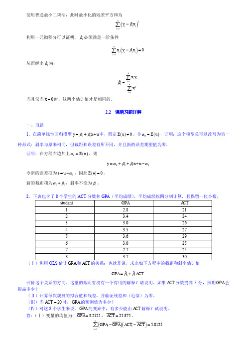
使用普通最小二乘法,此时最小化的残差平方和为()211niii y x β=-∑利用一元微积分可以证明,1β必须满足一阶条件()110niiii x y x β=-=∑从而解出1β为:1121ni ii nii x yxβ===∑∑当且仅当0x =时,这两个估计值才是相同的。
2.2 课后习题详解一、习题1.在简单线性回归模型01y x u ββ=++中,假定()0E u ≠。
令()0E u α=,证明:这个模型总可以改写为另一种形式:斜率与原来相同,但截距和误差有所不同,并且新的误差期望值为零。
证明:在方程右边加上()0E u α=,则0010y x u αββα=+++-令新的误差项为0e u α=-,因此()0E e =。
新的截距项为00αβ+,斜率不变为1β。
2(Ⅰ)利用OLS 估计GPA 和ACT 的关系;也就是说,求出如下方程中的截距和斜率估计值01ˆˆGPA ACT ββ=+^评价这个关系的方向。
这里的截距有没有一个有用的解释?请说明。
如果ACT 分数提高5分,预期GPA 会提高多少?(Ⅱ)计算每次观测的拟合值和残差,并验证残差和(近似)为零。
(Ⅲ)当20ACT =时,GPA 的预测值为多少?(Ⅳ)对这8个学生来说,GPA 的变异中,有多少能由ACT 解释?试说明。
答:(Ⅰ)变量的均值为: 3.2125GPA =,25.875ACT =。
()()15.8125niii GPA GPA ACT ACT =--=∑根据公式2.19可得:1ˆ 5.8125/56.8750.1022β==。
根据公式2.17可知:0ˆ 3.21250.102225.8750.5681β=-⨯=。
因此0.56810.1022GPA ACT =+^。
此处截距没有一个很好的解释,因为对样本而言,ACT 并不接近0。
如果ACT 分数提高5分,预期GPA 会提高0.1022×5=0.511。
(Ⅱ)每次观测的拟合值和残差表如表2-3所示:根据表可知,残差和为-0.002,忽略固有的舍入误差,残差和近似为零。
伍德里奇计量经济学第四章
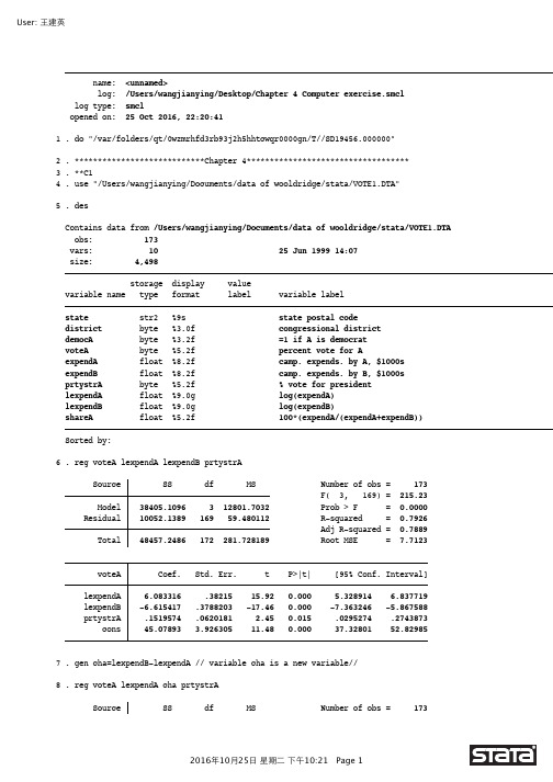
name: <unnamed>log: /Users/wangjianying/Desktop/Chapter 4 Computer exercise.smcl log type: smclopened on: 25 Oct 2016, 22:20:411. do "/var/folders/qt/0wzmrhfd3rb93j2h5hhtcwqr0000gn/T//SD19456.000000"2. ****************************Chapter 4***********************************3. **C14. use "/Users/wangjianying/Documents/data of wooldridge/stata/VOTE1.DTA"5. desContains data from /Users/wangjianying/Documents/data of wooldridge/stata/VOTE1.DTA obs: 173vars: 10 25 Jun 1999 14:07size: 4,498storage display valuevariable name type format label variable labelstate str2 %9s state postal codedistrict byte %3.0f congressional districtdemocA byte %3.2f =1 if A is democratvoteA byte %5.2f percent vote for AexpendA float %8.2f camp. expends. by A, $1000sexpendB float %8.2f camp. expends. by B, $1000sprtystrA byte %5.2f % vote for presidentlexpendA float %9.0g log(expendA)lexpendB float %9.0g log(expendB)shareA float %5.2f 100*(expendA/(expendA+expendB)) Sorted by:6. reg voteA lexpendA lexpendB prtystrASource SS df MS Number of obs = 173F( 3, 169) = 215.23 Model 38405.1096 3 12801.7032 Prob > F = 0.0000Residual 10052.1389 169 59.480112 R-squared = 0.7926Adj R-squared = 0.7889 Total 48457.2486 172 281.728189 Root MSE = 7.7123voteA Coef. Std. Err. t P>|t| [95% Conf. Interval] lexpendA 6.083316 .38215 15.92 0.000 5.328914 6.837719 lexpendB -6.615417 .3788203 -17.46 0.000 -7.363246 -5.867588 prtystrA .1519574 .0620181 2.45 0.015 .0295274 .2743873 _cons 45.07893 3.926305 11.48 0.000 37.32801 52.829857. gen cha=lexpendB-lexpendA // variable cha is a new variable//8. reg voteA lexpendA cha prtystrASource SS df MS Number of obs = 173F( 3, 169) = 215.23 Model 38405.1097 3 12801.7032 Prob > F = 0.0000Residual 10052.1388 169 59.4801115 R-squared = 0.7926Adj R-squared = 0.7889 Total 48457.2486 172 281.728189 Root MSE = 7.7123 voteA Coef. Std. Err. t P>|t| [95% Conf. Interval]lexpendA -.532101 .5330858 -1.00 0.320 -1.584466 .5202638cha -6.615417 .3788203 -17.46 0.000 -7.363246 -5.867588prtystrA .1519574 .0620181 2.45 0.015 .0295274 .2743873_cons 45.07893 3.926305 11.48 0.000 37.32801 52.829859. clear10.11. **C312. use "/Users/wangjianying/Documents/data of wooldridge/stata/hprice1.dta"13. desContains data from /Users/wangjianying/Documents/data of wooldridge/stata/hprice1.dta obs: 88vars: 10 17 Mar 2002 12:21size: 2,816storage display valuevariable name type format label variable labelprice float %9.0g house price, $1000sassess float %9.0g assessed value, $1000sbdrms byte %9.0g number of bdrmslotsize float %9.0g size of lot in square feetsqrft int %9.0g size of house in square feetcolonial byte %9.0g =1 if home is colonial stylelprice float %9.0g log(price)lassess float %9.0g log(assessllotsize float %9.0g log(lotsize)lsqrft float %9.0g log(sqrft)Sorted by:14. reg lprice sqrft bdrmsSource SS df MS Number of obs = 88F( 2, 85) = 60.73 Model 4.71671468 2 2.35835734 Prob > F = 0.0000Residual 3.30088884 85 .038833986 R-squared = 0.5883Adj R-squared = 0.5786 Total 8.01760352 87 .092156362 Root MSE = .19706 lprice Coef. Std. Err. t P>|t| [95% Conf. Interval]sqrft .0003794 .0000432 8.78 0.000 .0002935 .0004654bdrms .0288844 .0296433 0.97 0.333 -.0300543 .0878232_cons 4.766027 .0970445 49.11 0.000 4.573077 4.95897815. gen cha=sqrft-150*bdrms16. reg lprice cha bdrmsSource SS df MS Number of obs = 88F( 2, 85) = 60.73 Model 4.71671468 2 2.35835734 Prob > F = 0.0000Residual 3.30088884 85 .038833986 R-squared = 0.5883Adj R-squared = 0.5786 Total 8.01760352 87 .092156362 Root MSE = .19706lprice Coef. Std. Err. t P>|t| [95% Conf. Interval] cha .0003794 .0000432 8.78 0.000 .0002935 .0004654 bdrms .0858013 .0267675 3.21 0.002 .0325804 .1390223 _cons 4.766027 .0970445 49.11 0.000 4.573077 4.95897817. clear18.19. **C520. use "/Users/wangjianying/Documents/data of wooldridge/stata/MLB1.DTA"21. desContains data from /Users/wangjianying/Documents/data of wooldridge/stata/MLB1.DTA obs: 353vars: 47 16 Sep 1996 15:53size: 45,537storage display valuevariable name type format label variable labelsalary float %9.0g 1993 season salaryteamsal float %10.0f team payrollnl byte %9.0g =1 if national leagueyears byte %9.0g years in major leaguesgames int %9.0g career games playedatbats int %9.0g career at batsruns int %9.0g career runs scoredhits int %9.0g career hitsdoubles int %9.0g career doublestriples int %9.0g career tripleshruns int %9.0g career home runsrbis int %9.0g career runs batted inbavg float %9.0g career batting averagebb int %9.0g career walksso int %9.0g career strike outssbases int %9.0g career stolen basesfldperc int %9.0g career fielding percfrstbase byte %9.0g = 1 if first basescndbase byte %9.0g =1 if second baseshrtstop byte %9.0g =1 if shortstopthrdbase byte %9.0g =1 if third baseoutfield byte %9.0g =1 if outfieldcatcher byte %9.0g =1 if catcheryrsallst byte %9.0g years as all-starhispan byte %9.0g =1 if hispanicblack byte %9.0g =1 if blackwhitepop float %9.0g white pop. in cityblackpop float %9.0g black pop. in cityhisppop float %9.0g hispanic pop. in citypcinc int %9.0g city per capita incomegamesyr float %9.0g games per year in leaguehrunsyr float %9.0g home runs per yearatbatsyr float %9.0g at bats per yearallstar float %9.0g perc. of years an all-starslugavg float %9.0g career slugging averagerbisyr float %9.0g rbis per yearsbasesyr float %9.0g stolen bases per yearrunsyr float %9.0g runs scored per yearpercwhte float %9.0g percent white in citypercblck float %9.0g percent black in cityperchisp float %9.0g percent hispanic in cityblckpb float %9.0g black*percblckhispph float %9.0g hispan*perchispwhtepw float %9.0g white*percwhteblckph float %9.0g black*perchisphisppb float %9.0g hispan*percblcklsalary float %9.0g log(salary)Sorted by:22. reg lsalary years gamesyr bavg hrunsyrSource SS df MS Number of obs = 353F( 4, 348) = 145.24 Model 307.800674 4 76.9501684 Prob > F = 0.0000 Residual 184.374861 348 .52981282 R-squared = 0.6254Adj R-squared = 0.6211 Total 492.175535 352 1.39822595 Root MSE = .72788lsalary Coef. Std. Err. t P>|t| [95% Conf. Interval] years .0677325 .0121128 5.59 0.000 .0439089 .091556 gamesyr .0157595 .0015636 10.08 0.000 .0126841 .0188348 bavg .0014185 .0010658 1.33 0.184 -.0006776 .0035147 hrunsyr .0359434 .0072408 4.96 0.000 .0217021 .0501847 _cons 11.02091 .2657191 41.48 0.000 10.49829 11.5435323. reg lsalary years gamesyr bavg hrunsyr runsyr fldperc sbasesyrSource SS df MS Number of obs = 353F( 7, 345) = 87.25 Model 314.510478 7 44.9300682 Prob > F = 0.0000 Residual 177.665058 345 .514971181 R-squared = 0.6390Adj R-squared = 0.6317 Total 492.175535 352 1.39822595 Root MSE = .71761lsalary Coef. Std. Err. t P>|t| [95% Conf. Interval] years .0699848 .0119756 5.84 0.000 .0464305 .0935391 gamesyr .0078995 .0026775 2.95 0.003 .0026333 .0131657 bavg .0005296 .0011038 0.48 0.632 -.0016414 .0027007 hrunsyr .0232106 .0086392 2.69 0.008 .0062185 .0402027 runsyr .0173922 .0050641 3.43 0.001 .0074318 .0273525 fldperc .0010351 .0020046 0.52 0.606 -.0029077 .0049778 sbasesyr -.0064191 .0051842 -1.24 0.216 -.0166157 .0037775 _cons 10.40827 2.003255 5.20 0.000 6.468139 14.348424. test bavg fldperc sbasesyr( 1) bavg = 0( 2) fldperc = 0( 3) sbasesyr = 0F( 3, 345) = 0.69Prob > F = 0.561725. clear26. **C727. use "/Users/wangjianying/Documents/data of wooldridge/stata/twoyear.dta"28. sum phsrankVariable Obs Mean Std. Dev. Min Maxphsrank 6763 56.15703 24.27296 0 9929. reg lwage jc totcoll exper phsrankSource SS df MS Number of obs = 6763F( 4, 6758) = 483.85 Model 358.050568 4 89.5126419 Prob > F = 0.0000 Residual 1250.24552 6758 .185002297 R-squared = 0.2226Adj R-squared = 0.2222 Total 1608.29609 6762 .237843255 Root MSE = .43012 lwage Coef. Std. Err. t P>|t| [95% Conf. Interval] jc -.0093108 .0069693 -1.34 0.182 -.0229728 .0043512 totcoll .0754756 .0025588 29.50 0.000 .0704595 .0804918 exper .0049396 .0001575 31.36 0.000 .0046308 .0052483 phsrank .0003032 .0002389 1.27 0.204 -.0001651 .0007716 _cons 1.458747 .0236211 61.76 0.000 1.412442 1.50505230. reg lwage jc univ exper idSource SS df MS Number of obs = 6763F( 4, 6758) = 483.42 Model 357.807307 4 89.4518268 Prob > F = 0.0000 Residual 1250.48879 6758 .185038293 R-squared = 0.2225Adj R-squared = 0.2220 Total 1608.29609 6762 .237843255 Root MSE = .43016 lwage Coef. Std. Err. t P>|t| [95% Conf. Interval]jc .0666633 .0068294 9.76 0.000 .0532754 .0800511univ .0768813 .0023089 33.30 0.000 .0723552 .0814074exper .0049456 .0001575 31.40 0.000 .0046368 .0052543id 1.14e-07 2.09e-07 0.54 0.587 -2.97e-07 5.24e-07_cons 1.467533 .0228306 64.28 0.000 1.422778 1.51228831. reg lwage jc totcoll exper idSource SS df MS Number of obs = 6763F( 4, 6758) = 483.42 Model 357.807307 4 89.4518267 Prob > F = 0.0000Residual 1250.48879 6758 .185038293 R-squared = 0.2225Adj R-squared = 0.2220 Total 1608.29609 6762 .237843255 Root MSE = .43016 lwage Coef. Std. Err. t P>|t| [95% Conf. Interval]jc -.010218 .0069366 -1.47 0.141 -.023816 .00338totcoll .0768813 .0023089 33.30 0.000 .0723552 .0814074exper .0049456 .0001575 31.40 0.000 .0046368 .0052543id 1.14e-07 2.09e-07 0.54 0.587 -2.97e-07 5.24e-07_cons 1.467533 .0228306 64.28 0.000 1.422778 1.51228832. clear33. **C934. use "/Users/wangjianying/Documents/data of wooldridge/stata/discrim.dta"35. desContains data from /Users/wangjianying/Documents/data of wooldridge/stata/discrim.dta obs: 410vars: 37 8 Jan 2002 22:26size: 47,150storage display valuevariable name type format label variable labelpsoda float %9.0g price of medium soda, 1st wavepfries float %9.0g price of small fries, 1st wavepentree float %9.0g price entree (burger or chicken), 1st wave wagest float %9.0g starting wage, 1st wavenmgrs float %9.0g number of managers, 1st wavenregs byte %9.0g number of registers, 1st wavehrsopen float %9.0g hours open, 1st waveemp float %9.0g number of employees, 1st wavepsoda2 float %9.0g price of medium soday, 2nd wavepfries2 float %9.0g price of small fries, 2nd wavepentree2 float %9.0g price entree, 2nd wavewagest2 float %9.0g starting wage, 2nd wavenmgrs2 float %9.0g number of managers, 2nd wavenregs2 byte %9.0g number of registers, 2nd wavehrsopen2 float %9.0g hours open, 2nd waveemp2 float %9.0g number of employees, 2nd wavecompown byte %9.0g =1 if company ownedchain byte %9.0g BK = 1, KFC = 2, Roy Rogers = 3, Wendy's = 4 density float %9.0g population density, towncrmrte float %9.0g crime rate, townstate byte %9.0g NJ = 1, PA = 2prpblck float %9.0g proportion black, zipcodeprppov float %9.0g proportion in poverty, zipcodeprpncar float %9.0g proportion no car, zipcodehseval float %9.0g median housing value, zipcodenstores byte %9.0g number of stores, zipcodeincome float %9.0g median family income, zipcodecounty byte %9.0g county labellpsoda float %9.0g log(psoda)lpfries float %9.0g log(pfries)lhseval float %9.0g log(hseval)lincome float %9.0g log(income)ldensity float %9.0g log(density)NJ byte %9.0g =1 for New JerseyBK byte %9.0g =1 if Burger KingKFC byte %9.0g =1 if Kentucky Fried ChickenRR byte %9.0g =1 if Roy RogersSorted by:36. reg lpsoda prpblck lincome prppovSource SS df MS Number of obs = 401F( 3, 397) = 12.60 Model .250340622 3 .083446874 Prob > F = 0.0000Residual 2.62840943 397 .006620679 R-squared = 0.0870Adj R-squared = 0.0801 Total 2.87875005 400 .007196875 Root MSE = .08137 lpsoda Coef. Std. Err. t P>|t| [95% Conf. Interval]prpblck .0728072 .0306756 2.37 0.018 .0125003 .1331141lincome .1369553 .0267554 5.12 0.000 .0843552 .1895553prppov .38036 .1327903 2.86 0.004 .1192999 .6414201_cons -1.463333 .2937111 -4.98 0.000 -2.040756 -.885909237. corr lincome prppov(obs=409)lincome prppovlincome 1.0000prppov -0.8385 1.000038. reg lpsoda prpblck lincome prppov lhsevalSource SS df MS Number of obs = 401F( 4, 396) = 22.31 Model .529488085 4 .132372021 Prob > F = 0.0000 Residual 2.34926197 396 .00593248 R-squared = 0.1839Adj R-squared = 0.1757 Total 2.87875005 400 .007196875 Root MSE = .07702lpsoda Coef. Std. Err. t P>|t| [95% Conf. Interval] prpblck .0975502 .0292607 3.33 0.001 .0400244 .155076 lincome -.0529904 .0375261 -1.41 0.159 -.1267657 .0207848 prppov .0521229 .1344992 0.39 0.699 -.2122989 .3165447 lhseval .1213056 .0176841 6.86 0.000 .0865392 .1560721 _cons -.8415149 .2924318 -2.88 0.004 -1.416428 -.266601939. test lincome prppov( 1) lincome = 0( 2) prppov = 0F( 2, 396) = 3.52Prob > F = 0.030440.end of do-file41. log closename: <unnamed>log: /Users/wangjianying/Desktop/Chapter 4 Computer exercise.smcl log type: smclclosed on: 25 Oct 2016, 22:21:04。
学习笔记:伍德里奇《计量经济学》第五版-第三章 多元回归分析:估计
y = b 0+ b 1x 1+ b 2x 2+ . . . b k x k + u一、多元线性回归模型1.我们可以研究控制一些变量不变的条件下,其他变量对y的影响,而不是假定他们不相关。
Cons = b 0+ b 1inc+b 2inc 2 +u2.我们还能推广变量之间的函数关系如:通过在模型中包含更多的变量,我们更好的达到了SLR.4所表达的目的E(u|x 1,x 2, …,x k ) = 0 (3.8)HYP.1一般多元回归模型的关键假定(u和所有x都不相关):( )仍然是最小化残差和:对(3.12)求k +1次偏导得一阶条件(交给计算机计算)(此时假定k +1个方程只能得到估计值得唯一解2.1 如何得到OLS 估计值例3.1分析两个系数时,可得出当我们把其中一个因素涵盖在模型中时,另外一个因素的预测就变得不有力了1.系数表示局部效应(控制其他变量不变时,对y的效应)多元回归分析给了我们在收集不到“其他条件不变”时的数据仍有同样效果的能力2.“控制其他变量不变”的含义3.同时改变不止一个自变量(只需要将效应加和)2.2 对OLS 回归方程的解释从单变量情形加以推广,得:1.残差的样本平均值为02.每个自变量和OLS 残差之间的样本协方差为0。
因此OLS 拟合值和OLS 残差之间的样本协方差也为03.点总位于OLS 回归线上(性质1. 2.由一阶条件得,性质3.由1.可得2.3 OLS 的拟合值和残差( )其中 是x1对其他变量回归后的残差(即排除其他变量对x1的影响,类似矢量正交)2.4 对“排除其他变量影响”的解释( )(是 对 简单回归的斜率1.样本中x2对y的偏效应为0,即2.x1和x 2不相关,即(1. 2.可解释、 的差异由(3.23)知,在两种情况下利用矢量正交的理解考虑简单回归和两个自变量的回归:2.5简单回归和多元回归估计值比较可以证明,R2的另一种理解是 的实际值与其拟合值 的相关系数的平方,其中2.6 拟合优度(与简单回归大致相同)二、普通最小二乘法(多元线性回归模型的代数特征和对方程的解释)使用提示:1.该笔记是对伍德里奇《计量经济学》第五版第三章学习过程中的内容梳理2.由于本人水平有限,单独看该笔记估计会很吃力,且很可能出现错误,建议结合书本进行理解3.希望能够对想学习计量经济学的人起到一点点帮助第三章多元回归分析:估计2020年3月19日10:47由于定义下增加解释变量不会降低R2,所以判断一个解释变量是否应该放入模型的依据应该是该解释变量在总体中对y的偏效应是否非02.7 过原点的回归1.之前推导的性质不再成立,特别是OLS残差的样本平均值不再是02.计算R2没有特定的规则3.当截距项b0不等于0,斜率参数OLS估计量将有偏误;当截距项b0=0,估计带截距项方程的代价是,OLS斜率估计量的方差会更大2.8 OLS估计量的期望值MLR.1(线性于参数)MLR.2(随机抽样)MLR.3(不存在完全共线性,允许一定程度的相关)(在定义函数时要小心不要违背了MLR.3MLR.4(条件均值为0)(内生解释变量:解释变量可能与误差项相关定理3.1 OLS的无偏性()2.9 过度设定和设定不足(多了无关变量和少了解释变量)2.9.1过度设定(不影响OLS估计量的无偏性,但影响OLS估计量的方差)2.9.2设定不足1.简单情形:从一个斜率参数到两个斜率参数由(3.23):取均值得偏误为:(因此偏误的方向取决于两个符号,偏误的大小取决于两者之积,在应用中可以通过常识来判断偏误方向2.扩展情形:从两个斜率参数到三个斜率参数当你假设和不相关时,就可以证明和的关系和简单情形一样2.10 OLS估计量的方差MLR.5(同方差性,不仅可以简化公式,还得到了有效性)定理3.2 OLS斜率估计量的抽样方差在MLR.1-5下,以自变量的样本值为条件,有()(是的总样本波动,则是对所有其他自变量(并包含一个截距项)回归所得到的由(3.51)可知,估计量的抽样方差由三个要素决定:1.误差方差(噪声越大,越难估计)2.的总样本波动(越分散,越容易估计)3.自变量之间的线性关系(和其他自变量相关性越高,越不利于估计(很高的并不一定有问题,抽样方差的大小还要取决于剩下两个因素,可以通过收集更多的数据来削减多重共线性(当考虑某一个自变量 的方差时,若 和其他自变量均无关,那么其他自变量间的关系是不造成影响的,某些经济学家为了分离特定变量的因果效应,而在模型中包括许多控制因素,但这并不影响因果效应的证实( )当含有两个解释变量时:( )当含有一个解释变量时:((3.54)和(3.55)表明除非样本中x1和x2不相关,否则 <1.当 =0时,两个都无偏,但 < ,所以前者更好2.当不等于0时,不放x 2进去会导致有偏,放了x 2进去会导致方差增加,但我们喜欢把x2放进去的理由是:不放进去的偏误不会随着样本容量扩大而缩减,而放进去增加的方差却会随着样本容量的扩大逐渐缩小至0所以有两个结论:2.10.1 过度设定的方差(建立在过度设定无偏讨论的基础上)( )2.10.2 OLS 估计量的标准误(与简单回归相同)在假定MLR.1-5下,有(MLR .5若不满足(即异方差),会使标准误失效(第二种表达清楚说明了随着样本容量的扩大,在其他三项( 、 、 )都趋于常数的时候,估计量标准误是如何变小的因此得估计量的标准误:定理3.3 的无偏估计OLS 估计量是最优线性无偏估计量(如(3.22)所示的线性、无偏误、在线性无偏估计量中方差最小在MLR.1-5下,得定理3.4 高斯-马尔科夫定理2.11 对OLS 估计的一个正确认识。
伍德里奇计量经济学导论第6版笔记和课后习题答案

第1章计量经济学的性质与经济数据1.1复习笔记考点一:计量经济学★1计量经济学的含义计量经济学,又称经济计量学,是由经济理论、统计学和数学结合而成的一门经济学的分支学科,其研究内容是分析经济现象中客观存在的数量关系。
2计量经济学模型(1)模型分类模型是对现实生活现象的描述和模拟。
根据描述和模拟办法的不同,对模型进行分类,如表1-1所示。
(2)数理经济模型和计量经济学模型的区别①研究内容不同数理经济模型的研究内容是经济现象各因素之间的理论关系,计量经济学模型的研究内容是经济现象各因素之间的定量关系。
②描述和模拟办法不同数理经济模型的描述和模拟办法主要是确定性的数学形式,计量经济学模型的描述和模拟办法主要是随机性的数学形式。
③位置和作用不同数理经济模型可用于对研究对象的初步研究,计量经济学模型可用于对研究对象的深入研究。
考点二:经济数据★★★1经济数据的结构(见表1-3)2面板数据与混合横截面数据的比较(见表1-4)考点三:因果关系和其他条件不变★★1因果关系因果关系是指一个变量的变动将引起另一个变量的变动,这是经济分析中的重要目标之计量分析虽然能发现变量之间的相关关系,但是如果想要解释因果关系,还要排除模型本身存在因果互逆的可能,否则很难让人信服。
2其他条件不变其他条件不变是指在经济分析中,保持所有的其他变量不变。
“其他条件不变”这一假设在因果分析中具有重要作用。
1.2课后习题详解一、习题1.假设让你指挥一项研究,以确定较小的班级规模是否会提高四年级学生的成绩。
(i)如果你能指挥你想做的任何实验,你想做些什么?请具体说明。
(ii)更现实地,假设你能搜集到某个州几千名四年级学生的观测数据。
你能得到它们四年级班级规模和四年级末的标准化考试分数。
你为什么预计班级规模与考试成绩成负相关关系?(iii)负相关关系一定意味着较小的班级规模会导致更好的成绩吗?请解释。
答:(i)假定能够随机的分配学生们去不同规模的班级,也就是说,在不考虑学生诸如能力和家庭背景等特征的前提下,每个学生被随机的分配到不同的班级。
伍德里奇《计量经济学导论》(第4版)笔记和课后习题详解(2-8章)
使用普通最小二乘法,此时最小化的残差平方和为()211niii y x β=-∑利用一元微积分可以证明,1β必须满足一阶条件()110niiii x y x β=-=∑从而解出1β为:1121ni ii nii x yxβ===∑∑当且仅当0x =时,这两个估计值才是相同的。
2.2 课后习题详解一、习题1.在简单线性回归模型01y x u ββ=++中,假定()0E u ≠。
令()0E u α=,证明:这个模型总可以改写为另一种形式:斜率与原来相同,但截距和误差有所不同,并且新的误差期望值为零。
证明:在方程右边加上()0E u α=,则0010y x u αββα=+++-令新的误差项为0e u α=-,因此()0E e =。
新的截距项为00αβ+,斜率不变为1β。
2(Ⅰ)利用OLS 估计GPA 和ACT 的关系;也就是说,求出如下方程中的截距和斜率估计值01ˆˆGPA ACT ββ=+^评价这个关系的方向。
这里的截距有没有一个有用的解释?请说明。
如果ACT 分数提高5分,预期GPA 会提高多少?(Ⅱ)计算每次观测的拟合值和残差,并验证残差和(近似)为零。
(Ⅲ)当20ACT =时,GPA 的预测值为多少?(Ⅳ)对这8个学生来说,GPA 的变异中,有多少能由ACT 解释?试说明。
答:(Ⅰ)变量的均值为: 3.2125GPA =,25.875ACT =。
()()15.8125niii GPA GPA ACT ACT =--=∑根据公式2.19可得:1ˆ 5.8125/56.8750.1022β==。
根据公式2.17可知:0ˆ 3.21250.102225.8750.5681β=-⨯=。
因此0.56810.1022GPA ACT =+^。
此处截距没有一个很好的解释,因为对样本而言,ACT 并不接近0。
如果ACT 分数提高5分,预期GPA 会提高0.1022×5=0.511。
(Ⅱ)每次观测的拟合值和残差表如表2-3所示:根据表可知,残差和为-0.002,忽略固有的舍入误差,残差和近似为零。
伍德里奇计量经济学知识点总结

【伍德里奇计量经济学知识点总结】1. 基本概念伍德里奇计量经济学是指利用数学、统计学和计量经济学的方法对经济现象进行定量分析和预测的一门学科。
它是经济学的重要分支,通过建立数学模型和使用实证数据进行检验,可以揭示经济规律和进行政策分析。
2. 经典假定在伍德里奇计量经济学中,有一些经典的假定是非常重要的。
首先是线性假定,即假定经济关系是线性的;其次是随机抽样假定,即样本是随机抽取的,能够代表总体;还有就是无多重共线性、异方差和自相关等假定。
3. 模型建立在进行伍德里奇计量经济学的研究时,首先需要建立适当的计量经济模型。
常见的模型包括线性回归模型、多元回归模型、时间序列模型和横断面数据模型等。
在建立模型时,需要考虑模型的选择、变量的设定和函数形式的确定等问题。
4. 参数估计一旦模型建立完成,接下来就需要进行参数估计。
通常使用最小二乘法进行参数估计,通过最小化残差平方和来确定参数的估计值。
在进行参数估计时,需要考虑参数的一致性、有效性和假设检验等问题。
5. 模型诊断模型诊断是伍德里奇计量经济学中的重要环节,通过对模型的有效性、稳健性和适用性进行诊断,可以确保模型的准确性和可靠性。
模型诊断包括多重共线性、异方差、自相关和样本外验证等内容。
6. 预测和政策分析在进行伍德里奇计量经济学的研究时,需要对模型进行预测和政策分析。
通过对模型的预测能力和政策效应进行分析,可以为决策者提供重要的参考信息,并对经济现象进行深入理解和解释。
在我看来,伍德里奇计量经济学是一门非常有趣且重要的学科,它不仅可以帮助我们理解经济现象背后的规律,还可以为政策制定提供重要参考。
通过建立数学模型和使用实证数据进行检验,我们能够更加深入地探讨经济问题并作出合理的判断。
我也深刻意识到在进行伍德里奇计量经济学研究时,需要综合运用数学、统计学和经济学知识,这对我们的综合能力提出了更高的要求。
总结回顾起来,伍德里奇计量经济学是一门综合性强、逻辑性强的学科,在研究过程中需要我们对经济现象有着深刻的理解和分析能力。
伍德里奇《计量经济学导论》(第4版)笔记和课后习题详解-第5~9章【圣才出品】
βˆ1 的不一致性为:
plimβˆ1 β Cov x1,u /Var x1
圣才电子书 十万种考研考证电子书、题库视频学习平台
第 5 章 多元回归分析:OLS 的渐近性
5.1 复习笔记
一、一致性
1.定理 5.1:OLS 的一致性
在假定 MLR.1~MLR.4 下,对所有的 j=0,1,2,…,k,OLS 估计量 βˆ j 都是 βj 的一
致估计。
其次,零条件均值假定意味着已经正确地设定了总体回归函数(PRF)。也就是说,在 假定 MLR.4 下,可以得到解释变量对 y 的平均值或期望值的偏效应。如果只使用假定 MLR.4',那么,β0+β1x1+β2x2+…+βkxk 就不一定代表了总体回归函数,也就面临着 xj 的某些非线性函数可能与误差项相关的可能性。
三、OLSHale Waihona Puke 的渐近有效性4 / 162
圣才电子书
1.简单回归模型
标准正态分布在式中出现的方式与 tn-k-1 分布不同。这是因为这个分布只是一个近似。
实际上,由于随着自由度的变大,tn-k-1 趋近于标准正态分布,所以如下写法也是合理的:
βˆj βj
/ se
βˆ j
a
~ tnk 1
2.其他大样本检验:拉格朗日乘数统计量
(1)包含 k 个自变量的多元回归模型
①假定 MLR.4'是一个更自然的假定,因为它直接得到普通最小二乘估计值。
伍德里奇计量经济学导论第六版英文课件
伍德里奇计量经济学导论第六版英文课件Woodridge's Introduction to Econometrics, 6th Edition, is a comprehensive textbook that covers the fundamentals of econometrics in a clear and concise manner. The accompanying courseware is designed to help students further understand and apply the concepts discussed in the book.The courseware includes PowerPoint slides, practice quizzes, and interactive exercises to enhance students' learning experience. The slides cover the key topics in each chapter, providing visual aids to help students grasp complex concepts. The quizzes allow students to test their understanding of the material and receive immediate feedback on their performance. The interactive exercises provide hands-on practice withreal-world data sets, helping students develop their econometric skills.In addition to the courseware, students have access to online resources such as supplementary readings, video tutorials, and self-assessment tools. These resources are designed to support students in their learning journey and provide additional assistance when needed.Overall, Woodridge's Introduction to Econometrics, 6th Edition, is a valuable resource for students studying econometrics. The comprehensive courseware offers a range of tools to support students in their learning, making it easier for them to understand and apply the concepts discussed in the textbook. With its clear explanations and practical exercises, this courseware is an essential companion for students looking to excel in econometrics.。
伍德里奇《计量经济学》chap5
第5章 OLS 的渐近性(样本容量无限增大的情况:OLS 的大样本性质)5.1一致性(1) 依概率收敛定义 (2) 均方收敛定义 (3) 概率极限法则(4) 大数定律(弱大数定律,切比雪夫和辛钦) (5)一致性z 假定:MLR.1- MLR.4 z 不一致性:源于MLR.4不满足 简单回归模型 多元回归模型:一般而言,如果x1和u 相关,其他自变量x 都和u 无关,所有的1ˆβ……ˆkβ都是不一致的。
特殊情况:如果x1和u 相关,其他自变量x 都和u 无关,而且,其他自变量x和x1也无关,则只有1ˆβ是不一致的。
和偏误的比较:相似和区别(样本和总体的区别)5.2渐近正态性(作用:大样本情形下,可替代MLR.6假定)(1) 依分布收敛定义:符号d→,极限分布 (2) 中心极限定理(3) 渐近分布(来源于极限分布,又区别于极限分布),符号a∼z 假定:MLR.1- MLR.5同方差假定不成立,会如何?实际上渐近正态性仍然成立。
但是渐近方差计算方式改变,所以t 和F 分布要改变。
z 理解:当n →∞,ˆj β是均方收敛的,即收敛于期望,而且方差收敛于0。
但是,当n 是有限数时,n 很大的话,ˆjβ可近似看作服从正态分布,其方差还没有变为0,而是渐近方差。
见式5.7。
随着n →∞渐近方差的估计值,即se 是以1/n 的速度趋向于0的。
z 5.7式怎么来的?)12ˆijr −∑来5.3渐近有效性z 渐近有效性定义:“致,且渐近正态”的估计量,其渐近协方差阵小于等于任何一个一致且渐近正态的估计量的协方差阵,则它是渐近有效的。
z 格林P76:我们还没有在大样本中证明OLS 按照“任何”一种标准都是最优的。
定理5.3也不过是告诉我们:在某一类估计量中,OLS 是最优的,即渐近有效的。
伍德里奇《计量经济学导论》(第4版)笔记和课后习题详解(2-8章)
使用普通最小二乘法,此时最小化的残差平方和为()211niii y x β=-∑利用一元微积分可以证明,1β必须满足一阶条件()110niiii x y x β=-=∑从而解出1β为:1121ni ii nii x yxβ===∑∑当且仅当0x =时,这两个估计值才是相同的。
2.2 课后习题详解一、习题1.在简单线性回归模型01y x u ββ=++中,假定()0E u ≠。
令()0E u α=,证明:这个模型总可以改写为另一种形式:斜率与原来相同,但截距和误差有所不同,并且新的误差期望值为零。
证明:在方程右边加上()0E u α=,则0010y x u αββα=+++-令新的误差项为0e u α=-,因此()0E e =。
新的截距项为00αβ+,斜率不变为1β。
2(Ⅰ)利用OLS 估计GPA 和ACT 的关系;也就是说,求出如下方程中的截距和斜率估计值01ˆˆGPA ACT ββ=+^评价这个关系的方向。
这里的截距有没有一个有用的解释?请说明。
如果ACT 分数提高5分,预期GPA 会提高多少?(Ⅱ)计算每次观测的拟合值和残差,并验证残差和(近似)为零。
(Ⅲ)当20ACT =时,GPA 的预测值为多少?(Ⅳ)对这8个学生来说,GPA 的变异中,有多少能由ACT 解释?试说明。
答:(Ⅰ)变量的均值为: 3.2125GPA =,25.875ACT =。
()()15.8125niii GPA GPA ACT ACT =--=∑根据公式2.19可得:1ˆ 5.8125/56.8750.1022β==。
根据公式2.17可知:0ˆ 3.21250.102225.8750.5681β=-⨯=。
因此0.56810.1022GPA ACT =+^。
此处截距没有一个很好的解释,因为对样本而言,ACT 并不接近0。
如果ACT 分数提高5分,预期GPA 会提高0.1022×5=0.511。
(Ⅱ)每次观测的拟合值和残差表如表2-3所示:根据表可知,残差和为-0.002,忽略固有的舍入误差,残差和近似为零。
- 1、下载文档前请自行甄别文档内容的完整性,平台不提供额外的编辑、内容补充、找答案等附加服务。
- 2、"仅部分预览"的文档,不可在线预览部分如存在完整性等问题,可反馈申请退款(可完整预览的文档不适用该条件!)。
- 3、如文档侵犯您的权益,请联系客服反馈,我们会尽快为您处理(人工客服工作时间:9:00-18:30)。
CHAPTER1 TEACHINGNOTES YouhavesubstantiallatitudeaboutwhattoemphasizeinChapter1.Ifinditusefultotalkabouttheeconomicsofcrimeexample(Example1.1)andthewageexample(Example1.2)sothatstudentssee,attheoutset,thateconometricsislinkedtoeconomicreasoning,eveniftheeconomicsisnotcomplicatedtheory. Iliketofamiliarizestudentswiththeimportantdatastructuresthatempiricaleconomistsuse,focusingprimarilyoncross-sectionalandtimeseriesdatasets,asthesearewhatIcoverinafirst-semestercourse.Itisprobablyagoodideatomentionthegrowingimportanceofdatasetsthathavebothacross-sectionalandtimedimension. Ispendalmostanentirelecturetalkingabouttheproblemsinherentindrawingcausalinferencesinthesocialsciences.Idothismostlythroughtheagriculturalyield,returntoeducation,andcrimeexamples.Theseexamplesalsocontrastexperimentalandnonexperimental(observational)data.Studentsstudyingbusinessandfinancetendtofindthetermstructureofinterestratesexamplemorerelevant,althoughtheissuethereistestingtheimplicationofasimpletheory,asopposedtoinferringcausality.Ihavefoundthatspendingtimetalkingabouttheseexamples,inplaceofaformalreviewofprobabilityandstatistics,ismoresuccessful(andmoreenjoyableforthestudentsandme). CHAPTER2 TEACHINGNOTES ThisisthechapterwhereIexpectstudentstofollowmost,ifnotall,ofthealgebraicderivations.InclassIliketoderiveatleasttheunbiasednessoftheOLSslopecoefficient,andusuallyIderivethevariance.Ataminimum,Italkaboutthefactorsaffectingthevariance.Tosimplifythenotation,afterIemphasizetheassumptionsinthepopulationmodel,andassumerandomsampling,Ijustconditiononthevaluesoftheexplanatoryvariablesinthesample.Technically,thisisjustifiedbyrandomsamplingbecause,forexample,E(ui|x1,x2,…,xn)=E(ui|xi)byindependentsampling.IfindthatstudentsareabletofocusonthekeyassumptionSLR.4andsubsequentlytakemywordabouthowconditioningontheindependentvariablesinthesampleisharmless.(Ifyouprefer,theappendixtoChapter3doestheconditioningargumentcarefully.)Becausestatisticalinferenceisnomoredifficultinmultipleregressionthaninsimpleregression,IpostponeinferenceuntilChapter4.(Thisreducesredundancyandallowsyoutofocusontheinterpretivedifferencesbetweensimpleandmultipleregression.) Youmightnoticehow,comparedwithmostothertexts,IuserelativelyfewassumptionstoderivetheunbiasednessoftheOLSslopeestimator,followedbytheformulaforitsvariance.ThisisbecauseIdonotintroduceredundantorunnecessaryassumptions.Forexample,onceSLR.4isassumed,nothingfurtherabouttherelationshipbetweenuandxisneededtoobtaintheunbiasednessofOLSunderrandomsampling. CHAPTER3 TEACHINGNOTES Forundergraduates,Idonotworkthroughmostofthederivationsinthischapter,atleastnotindetail.Rather,Ifocusoninterpretingtheassumptions,whichmostlyconcernthepopulation.Otherthanrandomsampling,theonlyassumptionthatinvolvesmorethanpopulationconsiderationsistheassumptionaboutnoperfectcollinearity,wherethepossibilityofperfectcollinearityinthesample(evenifitdoesnotoccurinthepopulation)shouldbetouchedon.Themoreimportantissueisperfectcollinearityinthepopulation,butthisisfairlyeasytodispensewithviaexamples.Thesecomefrommyexperienceswiththekindsofmodelspecificationissuesthatbeginnershavetroublewith. Thecomparisonofsimpleandmultipleregressionestimates–basedontheparticularsampleathand,asopposedtotheirstatisticalproperties?–usuallymakesastrongimpression.SometimesIdonotbotherwiththe“partiallingout”interpretationofmultipleregression. Asfarasstatisticalproperties,noticehowItreattheproblemofincludinganirrelevantvariable:noseparatederivationisneeded,astheresultfollowsformTheorem3.1. Idoliketoderivetheomittedvariablebiasinthesimplecase.ThisisnotmuchmoredifficultthanshowingunbiasednessofOLSinthesimpleregressioncaseunderthefirstfourGauss-Markovassumptions.Itisimportanttogetth estudentsthinkingaboutthisproblemearlyon,andbeforetoomanyadditional(unnecessary)assumptionshavebeenintroduced. Ihaveintentionallykeptthediscussionofmulticollinearitytoaminimum.Thispartlyindicatesmybias,butitalsoreflectsreality.Itis,ofcourse,veryimportantforstudentstounderstandthepotentialconsequencesofhavinghighlycorrelatedindependentvariables.Butthisisoftenbeyondourcontrol,exceptthatwecanasklessofourmultipleregressionanalysis.Iftwoormoreexplanatoryvariablesarehighlycorrelatedinthesample,weshouldnotexpecttopreciselyestimatetheirceterisparibuseffectsinthepopulation. Ifindextensivetreatmentsofmulticollinearity,whereone“tests”orsomehow“solves”themulticollinearityproblem,tobemisleading,atbest.EventheorganizationofsometextsgivestheimpressionthatimperfectmulticollinearityissomehowaviolationoftheGauss-Markovassumptions:theyincludemulticollinearityinachapterorpartofthebookdevotedto“violationofthebasicassumptions,”orsomethinglikethat.Ihavenoticedthatmaster’sstudentswhohavehadsomeundergraduateeconometricsareoftenconfusedonthemulticollinearityissue.Itisveryimportantthatstudentsnotconfusemulticollinearityamongtheincludedexplanatoryvariablesinaregressionmodelwiththebiascausedbyomittinganimportantvariable. IdonotprovetheGauss-Markovtheorem.Instead,Iemphasizeitsimplications.Sometimes,andcertainlyforadvancedbeginners,IputaspecialcaseofProblem3.12onamidtermexam,whereImakeaparticularchoiceforthefunctiong(x).Ratherthanhavethestudentsdirectlycomparethevariances,theyshouldappealtotheGauss-MarkovtheoremforthesuperiorityofOLSoveranyotherlinear,unbiasedestimator. CHAPTER4 TEACHINGNOTES AtthestartofthischapterisgoodtimetoremindstudentsthataspecificerrordistributionplayednoroleintheresultsofChapter3.ThatisbecauseonlythefirsttwomomentswerederivedunderthefullsetofGauss-Markovassumptions.Nevertheless,normalityisneededtoobtainexactnormalsamplingdistributions(conditionalontheexplanatoryvariables).IemphasizethatthefullsetofCLMassumptionsareusedinthischapter,butthatinChapter5werelaxthenormalityassumptionandstillperformapproximatelyvalidinference.Onecouldarguethattheclassicallinearmodelresultscouldbeskippedentirely,andthatonlylarge-sampleanalysisisneeded.But,fromapracticalperspective,studentsstillneedtoknowwherethetdistributioncomesfrombecausevirtuallyallregressionpackagesreporttstatisticsandobtainp-valuesoffofthetdistribution.IthenfinditveryeasytocoverChapter5quickly,byjustsayingwecandropnormalityandstillusetstatisticsandtheassociatedp-valuesasbeingapproximatelyvalid.Besides,occasionallystudentswillhavetoanalyzesmallerdatasets,especiallyiftheydotheirownsmallsurveysforatermproject. Itiscrucialtoemphasizethatwetesthypothesesaboutunknownpopulationparameters.Itellmystudentsthat