伍德里奇计量经济学英文版各章总结
伍德里奇计量经济学第四章

伍德里奇计量经济学第四章name:log: /Users/wangjianying/Desktop/Chapter 4 Computer exercise.smcl log type: smclopened on: 25 Oct 2016, 22:20:411. do "/var/folders/qt/0wzmrhfd3rb93j2h5hhtcwqr0000gn/T//SD1945 6.000000"2. ****************************Chapter 4***********************************3. **C14. use "/Users/wangjianying/Documents/data of wooldridge/stata/VOTE1.DTA"5. desContains data from /Users/wangjianying/Documents/data of wooldridge/stata/VOTE1.DTA obs: 173vars: 10 25 Jun 1999 14:07size: 4,498storage display valuevariable name type format label variable labelstate str2 %9s state postal codedistrict byte %3.0f congressional districtdemocA byte %3.2f =1 if A is democratvoteA byte %5.2f percent vote for AexpendA float %8.2f camp. expends. by A, $1000sexpendB float %8.2f camp. expends. by B, $1000sprtystrA byte %5.2f % vote for presidentlexpendA float %9.0g log(expendA)lexpendB float %9.0g log(expendB)shareA float %5.2f 100*(expendA/(expendA+expendB)) Sorted by:6. reg voteA lexpendA lexpendB prtystrASource SS df MS Number of obs = 173F( 3, 169) = 215.23 Model 38405.1096 3 12801.7032 Prob > F = 0.0000Residual 10052.1389 169 59.480112 R-squared = 0.7926Adj R-squared = 0.7889 Total 48457.2486 172 281.728189 Root MSE = 7.7123voteA Coef. Std. Err. t P>|t| [95% Conf. Interval] lexpendA 6.083316 .38215 15.92 0.000 5.328914 6.837719 lexpendB -6.615417 .3788203 -17.46 0.000 -7.363246 -5.867588 prtystrA .1519574 .0620181 2.45 0.015 .0295274 .2743873 _cons 45.07893 3.926305 11.48 0.000 37.32801 52.829857. gen cha=lexpendB-lexpendA // variable cha is a new variable//8. reg voteA lexpendA cha prtystrASource SS df MS Number of obs = 173F( 3, 169) = 215.23 Model 38405.1097 3 12801.7032 Prob > F = 0.0000Residual 10052.1388 169 59.4801115 R-squared = 0.7926Adj R-squared = 0.7889 Total 48457.2486 172 281.728189 Root MSE = 7.7123 voteA Coef. Std. Err. t P>|t| [95% Conf. Interval] lexpendA -.532101 .5330858 -1.00 0.320 -1.584466 .5202638 cha -6.615417 .3788203 -17.46 0.000 -7.363246 -5.867588prtystrA .1519574 .0620181 2.45 0.015 .0295274 .2743873_cons 45.07893 3.926305 11.48 0.000 37.32801 52.829859. clear10.11. **C312. use "/Users/wangjianying/Documents/data of wooldridge/stata/hprice1.dta"13. desContains data from /Users/wangjianying/Documents/data of wooldridge/stata/hprice1.dta obs: 88vars: 10 17 Mar 2002 12:21size: 2,816storage display valuevariable name type format label variable labelprice float %9.0g house price, $1000sassess float %9.0g assessed value, $1000sbdrms byte %9.0g number of bdrmslotsize float %9.0g size of lot in square feetsqrft int %9.0g size of house in square feetcolonial byte %9.0g =1 if home is colonial stylelprice float %9.0g log(price)lassess float %9.0g log(assessllotsize float %9.0g log(lotsize)lsqrft float %9.0g log(sqrft)Sorted by:14. reg lprice sqrft bdrmsSource SS df MS Number of obs = 88F( 2, 85) = 60.73 Model 4.71671468 2 2.35835734 Prob > F = 0.0000Residual 3.30088884 85 .038833986 R-squared = 0.5883Adj R-squared = 0.5786 Total 8.01760352 87 .092156362 Root MSE = .19706 lprice Coef. Std. Err. t P>|t| [95% Conf. Interval] sqrft .0003794 .0000432 8.78 0.000 .0002935 .0004654bdrms .0288844 .0296433 0.97 0.333 -.0300543 .0878232_cons 4.766027 .0970445 49.11 0.000 4.573077 4.95897815. gen cha=sqrft-150*bdrms16. reg lprice cha bdrmsSource SS df MS Number of obs = 88F( 2, 85) = 60.73 Model 4.71671468 2 2.35835734 Prob > F = 0.0000Residual 3.30088884 85 .038833986 R-squared = 0.5883Adj R-squared = 0.5786 Total 8.01760352 87 .092156362 Root MSE = .19706lprice Coef. Std. Err. t P>|t| [95% Conf. Interval] cha .0003794 .0000432 8.78 0.000 .0002935 .0004654 bdrms .0858013 .0267675 3.21 0.002 .0325804 .1390223 _cons 4.766027 .0970445 49.11 0.000 4.573077 4.95897817. clear18.19. **C520. use "/Users/wangjianying/Documents/data of wooldridge/stata/MLB1.DTA"21. desContains data from /Users/wangjianying/Documents/data of wooldridge/stata/MLB1.DTA obs: 353vars: 47 16 Sep 1996 15:53size: 45,537storage display valuevariable name type format label variable labelsalary float %9.0g 1993 season salaryteamsal float %10.0f team payrollnl byte %9.0g =1 if national leagueyears byte %9.0g years in major leaguesgames int %9.0g career games playedatbats int %9.0g career at batsruns int %9.0g career runs scoredhits int %9.0g career hitsdoubles int %9.0g career doublestriples int %9.0g career tripleshruns int %9.0g career home runsrbis int %9.0g career runs batted inbavg float %9.0g career batting averagebb int %9.0g career walksso int %9.0g career strike outssbases int %9.0g career stolen basesfldperc int %9.0g career fielding perc frstbase byte %9.0g = 1 if first base scndbase byte %9.0g =1 if second base shrtstop byte %9.0g =1 if shortstop thrdbase byte %9.0g =1 if third base outfield byte %9.0g =1 if outfieldcatcher byte %9.0g =1 if catcheryrsallst byte %9.0g years as all-starhispan byte %9.0g =1 if hispanicblack byte %9.0g =1 if blackwhitepop float %9.0g white pop. in city blackpop float %9.0g black pop. in city hisppop float %9.0g hispanic pop. in city pcinc int %9.0g city per capita income gamesyr float %9.0g games per year in league hrunsyr float %9.0g home runs per year atbatsyr float %9.0g at bats per yearallstar float %9.0g perc. of years an all-star slugavg float %9.0g career slugging average rbisyr float %9.0g rbis per yearsbasesyr float %9.0g stolen bases per yearrunsyr float %9.0g runs scored per yearpercwhte float %9.0g percent white in citypercblck float %9.0g percent black in cityperchisp float %9.0g percent hispanic in cityblckpb float %9.0g black*percblckhispph float %9.0g hispan*perchispwhtepw float %9.0g white*percwhteblckph float %9.0g black*perchisphisppb float %9.0g hispan*percblcklsalary float %9.0g log(salary)Sorted by:22. reg lsalary years gamesyr bavg hrunsyrSource SS df MS Number of obs = 353F( 4, 348) = 145.24 Model 307.800674 4 76.9501684 Prob >F = 0.0000 Residual 184.374861 348 .52981282 R-squared =0.6254Adj R-squared = 0.6211 Total 492.175535 352 1.39822595 Root MSE = .72788lsalary Coef. Std. Err. t P>|t| [95% Conf. Interval] years .0677325 .0121128 5.59 0.000 .0439089 .091556 gamesyr .0157595 .0015636 10.08 0.000 .0126841 .0188348 bavg .0014185 .0010658 1.33 0.184 -.0006776 .0035147 hrunsyr .0359434 .0072408 4.96 0.000 .0217021 .0501847 _cons 11.02091 .2657191 41.48 0.000 10.49829 11.5435323. reg lsalary years gamesyr bavg hrunsyr runsyr fldperc sbasesyrSource SS df MS Number of obs = 353F( 7, 345) = 87.25 Model 314.510478 7 44.9300682 Prob > F = 0.0000 Residual 177.665058 345 .514971181 R-squared =0.6390Adj R-squared = 0.6317 Total 492.175535 352 1.39822595 Root MSE = .71761lsalary Coef. Std. Err. t P>|t| [95% Conf. Interval] years .0699848 .0119756 5.84 0.000 .0464305 .0935391 gamesyr .0078995 .0026775 2.95 0.003 .0026333 .0131657 bavg .0005296 .0011038 0.48 0.632 -.0016414 .0027007 hrunsyr .0232106 .0086392 2.69 0.008 .0062185 .0402027 runsyr .0173922 .0050641 3.43 0.001 .0074318 .0273525 fldperc .0010351 .0020046 0.52 0.606 -.0029077 .0049778 sbasesyr -.0064191 .0051842 -1.24 0.216 -.0166157 .0037775 _cons 10.40827 2.003255 5.20 0.000 6.468139 14.348424. test bavg fldperc sbasesyr( 1) bavg = 0( 2) fldperc = 0( 3) sbasesyr = 0F( 3, 345) = 0.69Prob > F = 0.561725. clear26. **C727. use "/Users/wangjianying/Documents/data of wooldridge/stata/twoyear.dta"28. sum phsrankVariable Obs Mean Std. Dev. Min Maxphsrank 6763 56.15703 24.27296 0 9929. reg lwage jc totcoll exper phsrankSource SS df MS Number of obs = 6763F( 4, 6758) = 483.85 Model 358.050568 4 89.5126419 Prob >F = 0.0000 Residual 1250.24552 6758 .185002297 R-squared =0.2226Adj R-squared = 0.2222 Total 1608.29609 6762 .237843255 Root MSE = .43012 lwage Coef. Std. Err. t P>|t| [95% Conf. Interval] jc -.0093108 .0069693 -1.34 0.182 -.0229728 .0043512 totcoll .0754756 .0025588 29.50 0.000 .0704595 .0804918 exper .0049396 .0001575 31.36 0.000 .0046308 .0052483 phsrank .0003032 .0002389 1.27 0.204 -.0001651 .0007716 _cons 1.458747 .0236211 61.76 0.000 1.412442 1.50505230. reg lwage jc univ exper idSource SS df MS Number of obs = 6763F( 4, 6758) = 483.42 Model 357.807307 4 89.4518268 Prob >F = 0.0000 Residual 1250.48879 6758 .185038293 R-squared =0.2225Adj R-squared = 0.2220 Total 1608.29609 6762 .237843255 Root MSE = .43016 lwage Coef. Std. Err. t P>|t| [95% Conf. Interval] jc .0666633 .0068294 9.76 0.000 .0532754 .0800511univ .0768813 .0023089 33.30 0.000 .0723552 .0814074exper .0049456 .0001575 31.40 0.000 .0046368 .0052543id 1.14e-07 2.09e-07 0.54 0.587 -2.97e-07 5.24e-07_cons 1.467533 .0228306 64.28 0.000 1.422778 1.51228831. reg lwage jc totcoll exper idSource SS df MS Number of obs = 6763F( 4, 6758) = 483.42 Model 357.807307 4 89.4518267 Prob > F = 0.0000Residual 1250.48879 6758 .185038293 R-squared = 0.2225 Adj R-squared = 0.2220 Total 1608.29609 6762 .237843255 Root MSE = .43016 lwage Coef. Std. Err. t P>|t| [95% Conf. Interval] jc -.010218 .0069366 -1.47 0.141 -.023816 .00338totcoll .0768813 .0023089 33.30 0.000 .0723552 .0814074exper .0049456 .0001575 31.40 0.000 .0046368 .0052543id 1.14e-07 2.09e-07 0.54 0.587 -2.97e-07 5.24e-07_cons 1.467533 .0228306 64.28 0.000 1.422778 1.51228832. clear33. **C934. use "/Users/wangjianying/Documents/data of wooldridge/stata/discrim.dta"35. desContains data from /Users/wangjianying/Documents/data of wooldridge/stata/discrim.dta obs: 410vars: 37 8 Jan 2002 22:26size: 47,150storage display valuevariable name type format label variable labelpsoda float %9.0g price of medium soda, 1st wavepfries float %9.0g price of small fries, 1st wavepentree float %9.0g price entree (burger or chicken), 1st wave wagest float %9.0g starting wage, 1st wavenmgrs float %9.0g number of managers, 1st wavenregs byte %9.0g number of registers, 1st wavehrsopen float %9.0g hours open, 1st waveemp float %9.0g number of employees, 1st wavepsoda2 float %9.0g price of medium soday, 2nd wavepfries2 float %9.0g price of small fries, 2nd wavepentree2 float %9.0g price entree, 2nd wavewagest2 float %9.0g starting wage, 2nd wavenmgrs2 float %9.0g number of managers, 2nd wavenregs2 byte %9.0g number of registers, 2nd wavehrsopen2 float %9.0g hours open, 2nd waveemp2 float %9.0g number of employees, 2nd wavecompown byte %9.0g =1 if company ownedchain byte %9.0g BK = 1, KFC = 2, Roy Rogers = 3, Wendy's= 4 density float %9.0g population density, towncrmrte float %9.0g crime rate, townstate byte %9.0g NJ = 1, PA = 2prpblck float %9.0g proportion black, zipcodeprppov float %9.0g proportion in poverty, zipcodeprpncar float %9.0g proportion no car, zipcodehseval float %9.0g median housing value, zipcodenstores byte %9.0g number of stores, zipcodeincome float %9.0g median family income, zipcodecounty byte %9.0g county labellpsoda float %9.0g log(psoda)lpfries float %9.0g log(pfries)lhseval float %9.0g log(hseval)lincome float %9.0g log(income)ldensity float %9.0g log(density)NJ byte %9.0g =1 for New JerseyBK byte %9.0g =1 if Burger KingKFC byte %9.0g =1 if Kentucky Fried ChickenRR byte %9.0g =1 if Roy RogersSorted by:36. reg lpsoda prpblck lincome prppovSource SS df MS Number of obs = 401F( 3, 397) = 12.60 Model .250340622 3 .083446874 Prob > F = 0.0000Residual 2.62840943 397 .006620679 R-squared = 0.0870Adj R-squared = 0.0801 Total 2.87875005 400 .007196875 Root MSE = .08137 lpsoda Coef. Std. Err. t P>|t| [95% Conf. Interval]prpblck .0728072 .0306756 2.37 0.018 .0125003 .1331141lincome .1369553 .0267554 5.12 0.000 .0843552 .1895553prppov .38036 .1327903 2.86 0.004 .1192999 .6414201_cons -1.463333 .2937111 -4.98 0.000 -2.040756 -.885909237. corr lincome prppov(obs=409)lincome prppovlincome 1.0000prppov -0.8385 1.000038. reg lpsoda prpblck lincome prppov lhsevalSource SS df MS Number of obs = 401F( 4, 396) = 22.31 Model .529488085 4 .132372021 Prob > F = 0.0000 Residual 2.34926197 396 .00593248 R-squared = 0.1839 Adj R-squared = 0.1757 Total 2.87875005 400 .007196875 Root MSE = .07702lpsoda Coef. Std. Err. t P>|t| [95% Conf. Interval] prpblck .0975502 .0292607 3.33 0.001 .0400244 .155076 lincome -.0529904 .0375261 -1.41 0.159 -.1267657 .0207848 prppov .0521229 .1344992 0.39 0.699 -.2122989 .3165447 lhseval .1213056 .0176841 6.86 0.000 .0865392 .1560721 _cons -.8415149 .2924318 -2.88 0.004 -1.416428 -.266601939. test lincome prppov( 1) lincome = 0( 2) prppov = 0F( 2, 396) = 3.52Prob > F = 0.030440.end of do-file41. log closename:log: /Users/wangjianying/Desktop/Chapter 4 Computer exercise.smcl log type: smclclosed on: 25 Oct 2016, 22:21:04。
计量经济学 伍德里奇 第一章

The main challenge of an impact evaluation is the construction of a suitable counterfactual situation.
An ideal experiment can be conducted to obtain the causal effect of fertilizer amount on yield when the levels of fertilizer are assigned to plots independently of other plot features that affect yield.
.12
.1
.08
unemployment rate
.06
.04
1976 1980
1985
1990
1995
2000
2005
Note: Shaded areas are times of recession following the definition of Elsby et al. (2009).
2010
Dandan Zhang (NSD)
Sep.-Dec. 2014 1 / 37
1. Introduction
Course Structure
1. Introduction (We4 Chapter 1) 2. Mathematical Foundations,Probability Theory (We4 Appendix B & C) 3. The Bivariate Linear Regression Model (We4 Chapter 2) 4. The Multivariate Linear Regression Model (We4 Chapter 3) 5. Inference (We4 Chapter 4) 6. Further Issues (We4 Chapter 6) 7. Multiple Regression Analysis with Qualitative Information (We4 Chapter 7) 8. Heteroscedasticity (We4 Chapter 8) 9. Specification and Data Issues (We4 Chapter 9) 10. Instrument variables (We4 Chapter 15) 11. Panel Data (We4 Chapter 14)
计量经济学课件英文版 伍德里奇
Two methods to estimate
2016/9/22 Department of Statistics-Zhaoliqin 17
Some Terminology, cont.
β0 :intercept parameter β1 :slope parameter means that a one-unit increase in x changes the expected value of y by the amount β1,holding the other factors in u fixed.
Department of Statistics-Zhaoliqin 16
2016/9/22
Some Terminology, cont.
y = β0 + β1x + u, E [u|x] = 0. β0 + β1x is the systematic part of y. u is the unsystematic part of y. u is denoted the error term. Other terms for u : error shock disturbance residual (sometimes in reference to fitted error term)
6
2016/9/22
Department of Statistics-Zhaoliqin
7
Hence, we are interested in studying is the mean of wages given the years of Education that will be denoted as E [Wages|Education] Following economic theory, we assume a specific model for E[Wages|Education]
伍德里奇计量经济学知识点总结

【伍德里奇计量经济学知识点总结】1. 基本概念伍德里奇计量经济学是指利用数学、统计学和计量经济学的方法对经济现象进行定量分析和预测的一门学科。
它是经济学的重要分支,通过建立数学模型和使用实证数据进行检验,可以揭示经济规律和进行政策分析。
2. 经典假定在伍德里奇计量经济学中,有一些经典的假定是非常重要的。
首先是线性假定,即假定经济关系是线性的;其次是随机抽样假定,即样本是随机抽取的,能够代表总体;还有就是无多重共线性、异方差和自相关等假定。
3. 模型建立在进行伍德里奇计量经济学的研究时,首先需要建立适当的计量经济模型。
常见的模型包括线性回归模型、多元回归模型、时间序列模型和横断面数据模型等。
在建立模型时,需要考虑模型的选择、变量的设定和函数形式的确定等问题。
4. 参数估计一旦模型建立完成,接下来就需要进行参数估计。
通常使用最小二乘法进行参数估计,通过最小化残差平方和来确定参数的估计值。
在进行参数估计时,需要考虑参数的一致性、有效性和假设检验等问题。
5. 模型诊断模型诊断是伍德里奇计量经济学中的重要环节,通过对模型的有效性、稳健性和适用性进行诊断,可以确保模型的准确性和可靠性。
模型诊断包括多重共线性、异方差、自相关和样本外验证等内容。
6. 预测和政策分析在进行伍德里奇计量经济学的研究时,需要对模型进行预测和政策分析。
通过对模型的预测能力和政策效应进行分析,可以为决策者提供重要的参考信息,并对经济现象进行深入理解和解释。
在我看来,伍德里奇计量经济学是一门非常有趣且重要的学科,它不仅可以帮助我们理解经济现象背后的规律,还可以为政策制定提供重要参考。
通过建立数学模型和使用实证数据进行检验,我们能够更加深入地探讨经济问题并作出合理的判断。
我也深刻意识到在进行伍德里奇计量经济学研究时,需要综合运用数学、统计学和经济学知识,这对我们的综合能力提出了更高的要求。
总结回顾起来,伍德里奇计量经济学是一门综合性强、逻辑性强的学科,在研究过程中需要我们对经济现象有着深刻的理解和分析能力。
伍德里奇《计量经济学导论》(第4版)笔记和课后习题详解-第5~9章【圣才出品】
βˆ1 的不一致性为:
plimβˆ1 β Cov x1,u /Var x1
圣才电子书 十万种考研考证电子书、题库视频学习平台
第 5 章 多元回归分析:OLS 的渐近性
5.1 复习笔记
一、一致性
1.定理 5.1:OLS 的一致性
在假定 MLR.1~MLR.4 下,对所有的 j=0,1,2,…,k,OLS 估计量 βˆ j 都是 βj 的一
致估计。
其次,零条件均值假定意味着已经正确地设定了总体回归函数(PRF)。也就是说,在 假定 MLR.4 下,可以得到解释变量对 y 的平均值或期望值的偏效应。如果只使用假定 MLR.4',那么,β0+β1x1+β2x2+…+βkxk 就不一定代表了总体回归函数,也就面临着 xj 的某些非线性函数可能与误差项相关的可能性。
三、OLSHale Waihona Puke 的渐近有效性4 / 162
圣才电子书
1.简单回归模型
标准正态分布在式中出现的方式与 tn-k-1 分布不同。这是因为这个分布只是一个近似。
实际上,由于随着自由度的变大,tn-k-1 趋近于标准正态分布,所以如下写法也是合理的:
βˆj βj
/ se
βˆ j
a
~ tnk 1
2.其他大样本检验:拉格朗日乘数统计量
(1)包含 k 个自变量的多元回归模型
①假定 MLR.4'是一个更自然的假定,因为它直接得到普通最小二乘估计值。
学习笔记:伍德里奇《计量经济学》第五版-第二章 简单回归模型
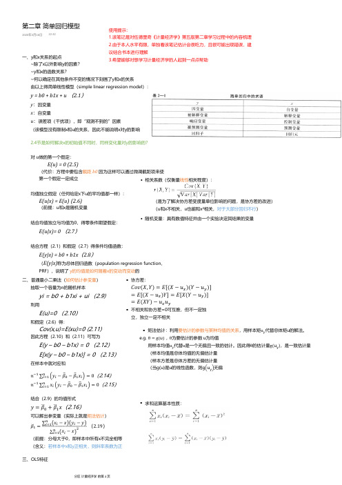
~除了x 以外影响y 的因素?~y 和x 的函数关系?~何以确定在其他条件不变的情况下刻画了y 和x 的关系由以上得简单线性模型(simple linear regression model ):y = b0+ b1x + u (2.1)y :因变量x :自变量u :误差项(干扰项),即“观测不到的”因素(该模型没有限制x 和u 的关系,因此不能说明x 对y 的影响2.4节是如何解决x 的初始值不同时,同样变化量对y 的影响的?E(u) = 0 (2.5)(代价:方程中要包含截距b0 因为这样可以通过微调截距项来使第一个假定一定成立对u 做的第一个假定:E(u|x) = E(u)(2.6)(前提:u 和x 是随机变量均值独立假定(任何给定x 下u 的平均值都一样):E(u|x)= 0 (2.7)结合均值独立与均值为0,得零条件期望假定:E(y|x) = b0 + b1x (2.8)(E(y|x)称为总体回归函数(population regression function ,PRF ),说明了y 的均值是如何随着x 的变动而变动的结合方程(2.1)和假定(2.7)得条件均值函数:一、y 和x关系的起点随机变量:具有数值特征并由一个实验决定其结果的变量•(是为了解决协方差受度量单位影响的问题,是协方差的改进)(u 和x 不相关,u 也能和x ²相关,对于大部分回归不行)相关系数(仅衡量线性相关程度):•yi = b0 + b1xi + ui (2.9)抽取一个容量为n 的随机样本E(u)=0 (2.10)利用Cov(x,u)=E(xu)=0 (2.11)和假定(2.6)得:E(y –b0 –b1x) = 0 (2.12)E[x(y –b0 –b1x)] = 0 (2.13)因此方程(2.10)和(2.11)可写为在样本中就对应和(2.14)(2.15)结合(2.9)的均值形式(2.16)可以解出参变量(实际上就是矩法估计)( )(前提:分母大于0,即样本中所有x 不完全相等(含义:若样本中x 和y 正相关,则斜率系数为正二、普通最小二乘法(如何估计参变量)协方差:•不相关和协方差=0可互推,但不一定独立,独立一定不相关•矩法估计:利用要估计的参数与某种均值的关系,用样本矩 代替总体矩u 的解法。
伍德里奇计量经济学导论第6版笔记和课后习题答案

第1章计量经济学的性质与经济数据1.1复习笔记考点一:计量经济学★1计量经济学的含义计量经济学,又称经济计量学,是由经济理论、统计学和数学结合而成的一门经济学的分支学科,其研究内容是分析经济现象中客观存在的数量关系。
2计量经济学模型(1)模型分类模型是对现实生活现象的描述和模拟。
根据描述和模拟办法的不同,对模型进行分类,如表1-1所示。
(2)数理经济模型和计量经济学模型的区别①研究内容不同数理经济模型的研究内容是经济现象各因素之间的理论关系,计量经济学模型的研究内容是经济现象各因素之间的定量关系。
②描述和模拟办法不同数理经济模型的描述和模拟办法主要是确定性的数学形式,计量经济学模型的描述和模拟办法主要是随机性的数学形式。
③位置和作用不同数理经济模型可用于对研究对象的初步研究,计量经济学模型可用于对研究对象的深入研究。
考点二:经济数据★★★1经济数据的结构(见表1-3)2面板数据与混合横截面数据的比较(见表1-4)考点三:因果关系和其他条件不变★★1因果关系因果关系是指一个变量的变动将引起另一个变量的变动,这是经济分析中的重要目标之计量分析虽然能发现变量之间的相关关系,但是如果想要解释因果关系,还要排除模型本身存在因果互逆的可能,否则很难让人信服。
2其他条件不变其他条件不变是指在经济分析中,保持所有的其他变量不变。
“其他条件不变”这一假设在因果分析中具有重要作用。
1.2课后习题详解一、习题1.假设让你指挥一项研究,以确定较小的班级规模是否会提高四年级学生的成绩。
(i)如果你能指挥你想做的任何实验,你想做些什么?请具体说明。
(ii)更现实地,假设你能搜集到某个州几千名四年级学生的观测数据。
你能得到它们四年级班级规模和四年级末的标准化考试分数。
你为什么预计班级规模与考试成绩成负相关关系?(iii)负相关关系一定意味着较小的班级规模会导致更好的成绩吗?请解释。
答:(i)假定能够随机的分配学生们去不同规模的班级,也就是说,在不考虑学生诸如能力和家庭背景等特征的前提下,每个学生被随机的分配到不同的班级。
伍德里奇计量经济学英文各章总结

CHAPTER 1TEACHING NOTESYou have substantial latitude about what to emphasize in Chapter 1.I find it useful to talk about the economics of crime example (Example and the wage example (Example so that students see, at the outset, that econometrics is linked to economic reasoning, even if the economics is not complicated theory.I like to familiarize students with the important data structures that empirical economists use, focusing primarily on cross-sectional and time series data sets, as these are what I cover in a first-semester course. It is probably a good idea to mention the growing importance of data sets that have both a cross-sectional and time dimension.I spend almost an entire lecture talking about the problems inherent in drawing causal inferences in the social sciences. I do this mostly through the agricultural yield, return to education, and crime examples. These examples also contrast experimental and nonexperimental (observational) data. Students studying business and finance tend to find the term structure of interest rates example more relevant, although the issue there is testing the implication of a simple theory, as opposed to inferring causality. I have found that spending time talking about these examples, in place of a formal review of probability and statistics, is more successful (and more enjoyable for the students and me).CHAPTER 2TEACHING NOTESThis is the chapter where I expect students to follow most, if not all, of the algebraic derivations. In class I like to derive at least the unbiasedness of the OLS slope coefficient, and usually I derive the variance. At a minimum, I talk about the factors affecting the variance. To simplify the notation, after I emphasize the assumptions in the population model, and assume random sampling, I just condition on the values of the explanatory variables in the sample. Technically, this is justified by random sampling because, for example, E(u i|x1,x2,…,x n) =E(u i|x i) by independent sampling. I find that students are able to focus on the key assumption and subsequently take my word about how conditioning on the independent variables in the sample is harmless. (If you prefer, the appendix to Chapter 3 does the conditioning argument carefully.) Because statistical inference is no more difficult in multiple regression than in simple regression, I postpone inference until Chapter 4. (This reduces redundancy and allows you to focus on the interpretive differences between simple and multiple regression.)You might notice how, compared with most other texts, I use relatively few assumptions to derive the unbiasedness of the OLS slope estimator, followed by the formula for its variance. This is because I do not introduce redundant or unnecessary assumptions. For example,once is assumed, nothing further about the relationship between u and x is needed to obtain the unbiasedness of OLS under random sampling.CHAPTER 3TEACHING NOTESFor undergraduates, I do not work through most of the derivations in this chapter, at least not in detail. Rather, I focus on interpreting the assumptions, which mostly concern the population. Other than random sampling, the only assumption that involves more than population considerations is the assumption about no perfect collinearity, where the possibility of perfect collinearity in the sample (even if it does not occur in the population) should be touched on. The more important issue is perfect collinearity in the population, but this is fairly easy to dispense with via examples. These come from my experiences with the kinds of model specification issues that beginners have trouble with.The comparison of simple and multiple regression estimates – based on the particular sample at hand, as opposed to their statistical properties – usually makes a strong impression. Sometimes I do not bother with the “partialling out” interpretation of multiple regression.As far as statistical properties, notice how I treat the problem of including an irrelevant variable: no separate derivation is needed, as the result follows form Theorem .I do like to derive the omitted variable bias in the simple case. This is not much more difficult than showing unbiasedness of OLS in the simple regression case under the first four Gauss-Markov assumptions. It is important to get the students thinking about this problem early on, and before too many additional (unnecessary) assumptions have been introduced.I have intentionally kept the discussion of multicollinearity to a minimum. This partly indicates my bias, but it also reflects reality. It is, of course, very important for students to understand the potential consequences of having highly correlated independent variables. But this is often beyond our control, except that we can ask less of our multiple regression analysis. If two or more explanatory variables are highly correlated in the sample, we should not expect to precisely estimate their ceteris paribus effects in the population.I find extensive treatments of multicollinearity, where one “tests” or somehow “solves” t he multicollinearity problem, to be misleading, at best. Even the organization of some texts gives the impression that imperfect multicollinearity is somehow a violation of the Gauss-Markov assumptions: they include multicollinearity in a chapter or part of the book devoted to “violation of the basic assumptions,” or something like that. I have noticed that master’s students who have had some undergraduate econometrics are often confused on the multicollinearityissue. It is very important that students not confuse multicollinearity among the included explanatory variables in a regression model with the bias caused by omitting an important variable.I do not prove the Gauss-Markov theorem. Instead, I emphasize its implications. Sometimes, and certainly for advanced beginners, I put a special case of Problem on a midterm exam, where I make a particular choice for the function g(x). Rather than have the students directly compare the variances, they should appeal to the Gauss-Markov theorem for the superiority of OLS over any other linear, unbiased estimator.CHAPTER 4TEACHING NOTESAt the start of this chapter is good time to remind students that a specific error distribution played no role in the results of Chapter 3. That is because only the first two moments were derived under the full set of Gauss-Markov assumptions. Nevertheless, normality is needed to obtain exact normal sampling distributions (conditional on the explanatory variables). I emphasize that the full set of CLM assumptions are used in this chapter, but that in Chapter 5 we relax the normality assumption and still perform approximately valid inference. One could argue that the classical linear model results could be skipped entirely, and that only large-sample analysis is needed. But, from a practicalperspective, students still need to know where the t distribution comes from because virtually all regression packages report t statistics and obtain p-values off of the t distribution. I then find it very easy to cover Chapter 5 quickly, by just saying we can drop normality and still use t statistics and the associated p-values as being approximately valid. Besides, occasionally students will have to analyze smaller data sets, especially if they do their own small surveys for a term project.It is crucial to emphasize that we test hypotheses about unknown population parameters. I tell my students that they will be punished ifˆ = 0 on an exam or, even worse, H0: .632 they write something like H0:1= 0.One useful feature of Chapter 4 is its illustration of how to rewrite a population model so that it contains the parameter of interest in testing a single restriction. I find this is easier, both theoretically and practically, than computing variances that can, in some cases, depend on numerous covariance terms. The example of testing equality of the return to two- and four-year colleges illustrates the basic method, and shows that the respecified model can have a useful interpretation. Of course, some statistical packages now provide a standard error for linear combinations of estimates with a simple command, and that should be taught, too.One can use an F test for single linear restrictions on multiple parameters, but this is less transparent than a t test and does notimmediately produce the standard error needed for a confidence interval or for testing a one-sided alternative. The trick of rewriting the population model is useful in several instances, including obtaining confidence intervals for predictions in Chapter 6, as well as for obtaining confidence intervals for marginal effects in models with interactions (also in Chapter 6).The major league baseball player salary example illustrates the difference between individual and joint significance when explanatory variables (rbisyr and hrunsyr in this case) are highly correlated. I tend to emphasize the R-squared form of the F statistic because, in practice, it is applicable a large percentage of the time, and it is much more readily computed. I do regret that this example is biased toward students in countries where baseball is played. Still, it is one of the better examples of multicollinearity that I have come across, and students of all backgrounds seem to get the point.CHAPTER 5TEACHING NOTESChapter 5 is short, but it is conceptually more difficult than the earlier chapters, primarily because it requires some knowledge of asymptotic properties of estimators. In class, I give a brief, heuristic description of consistency and asymptotic normality before stating the consistency and asymptotic normality of OLS. (Conveniently, the sameassumptions that work for finite sample analysis work for asymptotic analysis.) More advanced students can follow the proof of consistency of the slope coefficient in the bivariate regression case. Section contains a full matrix treatment of asymptotic analysis appropriate for a master’s level course.An explicit illustration of what happens to standard errors as the sample size grows emphasizes the importance of having a larger sample.I do not usually cover the LM statistic in a first-semester course, and I only briefly mention the asymptotic efficiency result. Without full use of matrix algebra combined with limit theorems for vectors and matrices, it is very difficult to prove asymptotic efficiency of OLS.I think the conclusions of this chapter are important for students to know, even though they may not fully grasp the details. On exams I usually include true-false type questions, with explanation, to test the stud ents’ understanding of asymptotics. [For example: “In large samples we do not have to worry about omitted variable bias.” (False). Or “Even if the error term is not normally distributed, in large samples we can still compute approximately valid confidence intervals under the Gauss-Markov assumptions.” (True).]CHAPTER6TEACHING NOTESI cover most of Chapter 6, but not all of the material in great detail.I use the example in Table to quickly run through the effects of data scaling on the important OLS statistics. (Students should already have a feel for the effects of data scaling on the coefficients, fitting values, and R-squared because it is covered in Chapter 2.) At most, I briefly mention beta coefficients; if students have a need for them, they can read this subsection.The functional form material is important, and I spend some time on more complicated models involving logarithms, quadratics, and interactions. An important point for models with quadratics, and especially interactions, is that we need to evaluate the partial effect at interesting values of the explanatory variables. Often, zero is not an interesting value for an explanatory variable and is well outside the range in the sample. Using the methods from Chapter 4, it is easy to obtain confidence intervals for the effects at interesting x values.As far as goodness-of-fit, I only introduce the adjusted R-squared, as I think using a slew of goodness-of-fit measures to choose a model can be confusing to novices (and does not reflect empirical practice). It is important to discuss how, if we fixate on a high R-squared, we may wind up with a model that has no interesting ceteris paribus interpretation.I often have students and colleagues ask if there is a simple way to predict y when log(y) has been used as the dependent variable, and to obtain a goodness-of-fit measure for the log(y) model that can be compared with the usual R-squared obtained when y is the dependent variable. The methods described in Section are easy to implement and, unlike other approaches, do not require normality.The section on prediction and residual analysis contains several important topics, including constructing prediction intervals. It is useful to see how much wider the prediction intervals are than the confidence interval for the conditional mean. I usually discuss some of the residual-analysis examples, as they have real-world applicability.CHAPTER 7TEACHING NOTESThis is a fairly standard chapter on using qualitative information in regression analysis, although I try to emphasize examples with policy relevance (and only cross-sectional applications are included.).In allowing for different slopes, it is important, as in Chapter 6, to appropriately interpret the parameters and to decide whether they are of direct interest. For example, in the wage equation where the return to education is allowed to depend on gender, the coefficient on the female dummy variable is the wage differential between women and men at zero years of education. It is not surprising that we cannot estimatethis very well, nor should we want to. In this particular example we would drop the interaction term because it is insignificant, but the issue of interpreting the parameters can arise in models where the interaction term is significant.In discussing the Chow test, I think it is important to discuss testing for differences in slope coefficients after allowing for an intercept difference. In many applications, a significant Chow statistic simply indicates intercept differences. (See the example in Section on student-athlete GPAs in the text.) From a practical perspective, it is important to know whether the partial effects differ across groups or whether a constant differential is sufficient.I admit that an unconventional feature of this chapter is its introduction of the linear probability model. I cover the LPM here for several reasons. First, the LPM is being used more and more because it is easier to interpret than probit or logit models. Plus, once the proper parameter scalings are done for probit and logit, the estimated effects are often similar to the LPM partial effects near the mean or median values of the explanatory variables. The theoretical drawbacks of the LPM are often of secondary importance in practice. Computer Exercise is a good one to illustrate that, even with over 9,000 observations, the LPM can deliver fitted values strictly between zero and one for all observations.If the LPM is not covered, many students will never know about using econometrics to explain qualitative outcomes. This would be especially unfortunate for students who might need to read an article where an LPM is used, or who might want to estimate an LPM for a term paper or senior thesis. Once they are introduced to purpose and interpretation of the LPM, along with its shortcomings, they can tackle nonlinear models on their own or in a subsequent course.A useful modification of the LPM estimated in equation is to drop kidsge6 (because it is not significant) and then define two dummy variables, one for kidslt6 equal to one and the other for kidslt6 at least two. These can be included in place of kidslt6 (with no young children being the base group). This allows a diminishing marginal effect in an LPM. I was a bit surprised when a diminishing effect did not materialize.CHAPTER 8TEACHING NOTESThis is a good place to remind students that homoskedasticity played no role in showing that OLS is unbiased for the parameters in the regression equation. In addition, you probably should mention that there is nothing wrong with the R-squared or adjusted R-squared as goodness-of-fit measures. The key is that these are estimates of the population R-squared, 1 – [Var(u)/Var(y)], where the variances are the unconditional variances in the population. The usual R-squared, andthe adjusted version, consistently estimate the population R-squared whether or not Var(u|x) = Var(y|x) depends on x. Of course, heteroskedasticity causes the usual standard errors, t statistics, and F statistics to be invalid, even in large samples, with or without normality.By explicitly stating the homoskedasticity assumption as conditional on the explanatory variables that appear in the conditional mean, it is clear that only heteroskedasticity that depends on the explanatory variables in the model affects the validity of standard errors and test statistics. The version of the Breusch-Pagan test in the text, and the White test, are ideally suited for detecting forms of heteroskedasticity that invalidate inference obtained under homoskedasticity. If heteroskedasticity depends on an exogenous variable that does not also appear in the mean equation, this can be exploited in weighted least squares for efficiency, but only rarely is such a variable available. One case where such a variable is available is when an individual-level equation has been aggregated. I discuss this case in the text but I rarely have time to teach it.As I mention in the text, other traditional tests for heteroskedasticity, such as the Park and Glejser tests, do not directly test what we want, or add too many assumptions under the null. The Goldfeld-Quandt test only works when there is a natural way to order thedata based on one independent variable. This is rare in practice, especially for cross-sectional applications.Some argue that weighted least squares estimation is a relic, and is no longer necessary given the availability of heteroskedasticity-robust standard errors and test statistics. While I am sympathetic to this argument, it presumes that we do not care much about efficiency. Even in large samples, the OLS estimates may not be precise enough to learn much about the population parameters. With substantial heteroskedasticity we might do better with weighted least squares, even if the weighting function is misspecified. As discussed in the text on pages 288-289, one can, and probably should, compute robust standard errors after weighted least squares. For asymptotic efficiency comparisons, these would be directly comparable to the heteroskedasiticity-robust standard errors for OLS.Weighted least squares estimation of the LPM is a nice example of feasible GLS, at least when all fitted values are in the unit interval. Interestingly, in the LPM examples in the text and the LPM computer exercises, the heteroskedasticity-robust standard errors often differ by only small amounts from the usual standard errors. However, in a couple of cases the differences are notable, as in Computer Exercise .CHAPTER 9TEACHING NOTESThe coverage of RESET in this chapter recognizes that it is a test for neglected nonlinearities, and it should not be expected to be more than that. (Formally, it can be shown that if an omitted variable has a conditional mean that is linear in the included explanatory variables, RESET has no ability to detect the omitted variable. Interested readers may consult my chapter in Companion to Theoretical Econometrics, 2001, edited by Badi Baltagi.) I just teach students the F statistic version of the test.The Davidson-MacKinnon test can be useful for detecting functional form misspecification, especially when one has in mind a specific alternative, nonnested model. It has the advantage of always being a one degree of freedom test.I think the proxy variable material is important, but the main points can be made with Examples and . The first shows that controlling for IQ can substantially change the estimated return to education, and the omitted ability bias is in the expected direction. Interestingly, education and ability do not appear to have an interactive effect. Example is a nice example of how controlling for a previous value of the dependent variable – something that is often possible with survey and nonsurvey data – can greatly affect a policy conclusion. Computer Exercise is also a good illustration of this method.I rarely get to teach the measurement error material, although the attenuation bias result for classical errors-in-variables is worth mentioning.The result on exogenous sample selection is easy to discuss, with more details given in Chapter 17. The effects of outliers can be illustrated using the examples. I think the infant mortality example, Example , is useful for illustrating how a single influential observation can have a large effect on the OLS estimates.With the growing importance of least absolute deviations, it makes sense to at least discuss the merits of LAD, at least in more advanced courses. Computer Exercise is a good example to show how mean and median effects can be very different, even though there may not be “outliers” in the usual sense.CHAPTER 10TEACHING NOTESBecause of its realism and its care in stating assumptions, this chapter puts a somewhat heavier burden on the instructor and student than traditional treatments of time series regression. Nevertheless, I think it is worth it. It is important that students learn that there are potential pitfalls inherent in using regression with time series data that are not present for cross-sectional applications. Trends, seasonality, and high persistence are ubiquitous in time series data. By this time,students should have a firm grasp of multiple regression mechanics and inference, and so you can focus on those features that make time series applications different from cross-sectional ones.I think it is useful to discuss static and finite distributed lag models at the same time, as these at least have a shot at satisfying theGauss-Markov assumptions. Many interesting examples have distributed lag dynamics. In discussing the time series versions of the CLM assumptions, I rely mostly on intuition. The notion of strict exogeneity is easy to discuss in terms of feedback. It is also pretty apparent that, in many applications, there are likely to be some explanatory variables that are not strictly exogenous. What the student should know is that, to conclude that OLS is unbiased – as opposed to consistent – we need to assume a very strong form of exogeneity of the regressors. Chapter 11 shows that only contemporaneous exogeneity is needed for consistency.Although the text is careful in stating the assumptions, in class, after discussing strict exogeneity, I leave the conditioning on X implicit, especially when I discuss the no serial correlation assumption. As this is a new assumption I spend some time on it. (I also discuss why we did not need it for random sampling.)Once the unbiasedness of OLS, the Gauss-Markov theorem, and the sampling distributions under the classical linear model assumptions havebeen covered – which can be done rather quickly – I focus on applications. Fortunately, the students already know about logarithms and dummy variables. I treat index numbers in this chapter because they arise in many time series examples.A novel feature of the text is the discussion of how to compute goodness-of-fit measures with a trending or seasonal dependent variable. While detrending or deseasonalizing y is hardly perfect (and does not work with integrated processes), it is better than simply reporting the very high R-squareds that often come with time series regressions with trending variables.CHAPTER 11TEACHING NOTESMuch of the material in this chapter is usually postponed, or not covered at all, in an introductory course. However, as Chapter 10 indicates, the set of time series applications that satisfy all of the classical linear model assumptions might be very small. In my experience, spurious time series regressions are the hallmark of many student projects that use time series data. Therefore, students need to be alerted to the dangers of using highly persistent processes in time series regression equations. (Spurious regression problem and the notion of cointegration are covered in detail in Chapter 18.)It is fairly easy to heuristically describe the difference between a weakly dependent process and an integrated process. Using the MA(1) and the stable AR(1) examples is usually sufficient.When the data are weakly dependent and the explanatory variables are contemporaneously exogenous, OLS is consistent. This result has many applications, including the stable AR(1) regression model. When we add the appropriate homoskedasticity and no serial correlation assumptions, the usual test statistics are asymptotically valid.The random walk process is a good example of a unit root (highly persistent) process. In a one-semester course, the issue comes down to whether or not to first difference the data before specifying the linear model. While unit root tests are covered in Chapter 18, just computing the first-order autocorrelation is often sufficient, perhaps after detrending. The examples in Section illustrate how differentfirst-difference results can be from estimating equations in levels.Section is novel in an introductory text, and simply points out that, if a model is dynamically complete in a well-defined sense, it should not have serial correlation. Therefore, we need not worry about serial correlation when, say, we test the efficient market hypothesis. Section further investigates the homoskedasticity assumption, and, in a time series context, emphasizes that what is contained in the explanatory variables determines what kind of heteroskedasticity is ruled out by theusual OLS inference. These two sections could be skipped without loss of continuity.CHAPTER 12TEACHING NOTESMost of this chapter deals with serial correlation, but it also explicitly considers heteroskedasticity in time series regressions. The first section allows a review of what assumptions were needed to obtain both finite sample and asymptotic results. Just as with heteroskedasticity, serial correlation itself does not invalidate R-squared. In fact, if the data are stationary and weakly dependent, R-squared and adjusted R-squared consistently estimate the population R-squared (which is well-defined under stationarity).Equation is useful for explaining why the usual OLS standard errors are not generally valid with AR(1) serial correlation. It also provides a good starting point for discussing serial correlation-robust standard errors in Section . The subsection on serial correlation with lagged dependent variables is included to debunk the myth that OLS is always inconsistent with lagged dependent variables and serial correlation. I do not teach it to undergraduates, but I do to master’s students.Section is somewhat untraditional in that it begins with an asymptotic t test for AR(1) serial correlation (under strict exogeneity of the regressors). It may seem heretical not to give the Durbin-Watsonstatistic its usual prominence, but I do believe the DW test is less useful than the t test. With nonstrictly exogenous regressors I cover only the regression form of Durbin’s test, as the h statistic is asymptotically equivalent and not always computable.Section , on GLS and FGLS estimation, is fairly standard, although I try to show how comparing OLS estimates and FGLS estimates is not so straightforward. Unfortunately, at the beginning level (and even beyond), it is difficult to choose a course of action when they are very different.I do not usually cover Section in a first-semester course, but, because some econometrics packages routinely compute fully robust standard errors, students can be pointed to Section if they need to learn something about what the corrections do. I do cover Section for a master’s level course in applied econometrics (after the first-semester course).I also do not cover Section in class; again, this is more to serve as a reference for more advanced students, particularly those with interests in finance. One important point is that ARCH is heteroskedasticity and not serial correlation, something that is confusing in many texts. If a model contains no serial correlation, the usual heteroskedasticity-robust statistics are valid. I have a brief subsection on correcting for a known。
- 1、下载文档前请自行甄别文档内容的完整性,平台不提供额外的编辑、内容补充、找答案等附加服务。
- 2、"仅部分预览"的文档,不可在线预览部分如存在完整性等问题,可反馈申请退款(可完整预览的文档不适用该条件!)。
- 3、如文档侵犯您的权益,请联系客服反馈,我们会尽快为您处理(人工客服工作时间:9:00-18:30)。
CHAPTER 1TEACHING NOTESYou have substantial latitude about what to emphasize in Chapter 1. I find it useful to talk about the economics of crime example (Example 1.1) and the wage example (Example 1.2) so that students see, at the outset, that econometrics is linked to economic reasoning, even if the economics is not complicated theory.I like to familiarize students with the important data structures that empirical economists use, focusing primarily on cross-sectional and time series data sets, as these are what I cover in a first-semester course. It is probably a good idea to mention the growing importance of data sets that have both a cross-sectional and time dimension.I spend almost an entire lecture talking about the problems inherent in drawing causal inferences in the social sciences. I do this mostly through the agricultural yield, return to education, and crime examples. These examples also contrast experimental and nonexperimental (observational) data. Students studying business and finance tend to find the term structure of interest rates example more relevant, although the issue there is testing the implication of a simple theory, as opposed to inferring causality. I have found that spending time talking about these examples, in place of a formal review of probability and statistics, is more successful (and more enjoyable for the students and me).CHAPTER 2TEACHING NOTESThis is the chapter where I expect students to follow most, if not all, of the algebraic derivations. In class I like to derive at least the unbiasedness of the OLS slope coefficient, and usually I derive the variance. At a minimum, I talk about the factors affecting the variance. To simplify the notation, after I emphasize the assumptions in the population model, and assume random sampling, I just condition on the values of the explanatory variables in the sample. Technically, this is justified by random sampling because, for example, E(u i|x1,x2,…,x n) = E(u i|x i) by independent sampling. I find that students are able to focus on the key assumption SLR.4 and subsequently take my word about how conditioning on the independent variables in the sample is harmless. (If you prefer, the appendix to Chapter 3 does the conditioning argument carefully.) Because statistical inference is no more difficult in multiple regression than in simple regression, I postpone inference until Chapter 4. (This reduces redundancy and allows you to focus on the interpretive differences between simple and multiple regression.)You might notice how, compared with most other texts, I use relatively few assumptions to derive the unbiasedness of the OLS slope estimator, followed by the formula for its variance. This is because I do not introduce redundant or unnecessary assumptions. For example, once SLR.4 is assumed, nothing further about the relationship between u and x is needed to obtain the unbiasedness of OLS under random sampling.CHAPTER 3TEACHING NOTESFor undergraduates, I do not work through most of the derivations in this chapter, at least not in detail. Rather, I focus on interpreting the assumptions, which mostly concern the population. Other than random sampling, the only assumption that involves more than population considerations is the assumption about no perfect collinearity, where the possibility of perfect collinearity in the sample (even if it does not occur in the population) should be touched on. The more important issue is perfect collinearity in the population, but this is fairly easy to dispense with via examples. These come from my experiences with the kinds of model specification issues that beginners have trouble with.The comparison of simple and multiple regression estimates – based on the particular sample at hand, as opposed to their statistical properties – usually makes a strong impression. Sometimes I do not bother with the “partialling out” interpretation of multiple regression.As far as statistical properties, notice how I treat the problem of including an irrelevant variable: no separate derivation is needed, as the result follows form Theorem 3.1.I do like to derive the omitted variable bias in the simple case. This is not much more difficult than showing unbiasedness of OLS in the simple regression case under the first four Gauss-Markov assumptions. It is important to get the students thinking about this problem early on, and before too many additional (unnecessary) assumptions have been introduced.I have intentionally kept the discussion of multicollinearity to a minimum. This partly indicates my bias, but it also reflects reality. It is, of course, very important for students to understand the potential consequences of having highly correlated independent variables. But this is often beyond our control, except that we can ask less of our multiple regression analysis. If two or more explanatory variables are highly correlated in the sample, we should not expect to precisely estimate their ceteris paribus effects in the population.I find extensive treatments of multicollinearity, where one “tests” or somehow “solves” the multicollinearity problem, to be misleading, at best. Even the organization of some texts gives the impression that imperfect multicollinearity is somehow a violation of the Gauss-Markov assumptions: they include multicollinearity in a chapter or part of the book devoted to “violation of the basic assumptions,” or something like that. I have noticed that master’s students who have had some undergraduate econometrics are often confused on the multicollinearity issue. It is very important that students not confuse multicollinearity among the included explanatory variables in a regression model with the bias caused by omitting an important variable.I do not prove the Gauss-Markov theorem. Instead, I emphasize its implications. Sometimes, and certainly for advanced beginners, I put a special case of Problem 3.12 on a midterm exam, where I make a particular choice for the function g(x). Rather than have the students directly compare the variances, they shouldappeal to the Gauss-Markov theorem for the superiority of OLS over any other linear, unbiased estimator.CHAPTER 4TEACHING NOTESAt the start of this chapter is good time to remind students that a specific error distribution played no role in the results of Chapter 3. That is because only the first two moments were derived under the full set of Gauss-Markov assumptions. Nevertheless, normality is needed to obtain exact normal sampling distributions (conditional on the explanatory variables). I emphasize that the full set of CLM assumptions are used in this chapter, but that in Chapter 5 we relax the normality assumption and still perform approximately valid inference. One could argue that the classical linear model results could be skipped entirely, and that only large-sample analysis is needed. But, from a practical perspective, students still need to know where the t distribution comes from because virtually all regression packages report t statistics and obtain p -values off of the t distribution. I then find it very easy tocover Chapter 5 quickly, by just saying we can drop normality and still use t statistics and the associated p -values as being approximately valid. Besides, occasionally students will have to analyze smaller data sets, especially if they do their own small surveys for a term project.It is crucial to emphasize that we test hypotheses about unknown population parameters. I tell my students that they will be punished if they write something likeH 0:1ˆ = 0 on an exam or, even worse, H 0: .632 = 0. One useful feature of Chapter 4 is its illustration of how to rewrite a population model so that it contains the parameter of interest in testing a single restriction. I find this is easier, both theoretically and practically, than computing variances that can, in some cases, depend on numerous covariance terms. The example of testing equality of the return to two- and four-year colleges illustrates the basic method, and shows that the respecified model can have a useful interpretation. Of course, some statistical packages now provide a standard error for linear combinations of estimates with a simple command, and that should be taught, too.One can use an F test for single linear restrictions on multiple parameters, but this is less transparent than a t test and does not immediately produce the standard error needed for a confidence interval or for testing a one-sided alternative. The trick of rewriting the population model is useful in several instances, including obtaining confidence intervals for predictions in Chapter 6, as well as for obtaining confidence intervals for marginal effects in models with interactions (also in Chapter6).The major league baseball player salary example illustrates the differencebetween individual and joint significance when explanatory variables (rbisyr and hrunsyr in this case) are highly correlated. I tend to emphasize the R -squared form of the F statistic because, in practice, it is applicable a large percentage of the time, and it is much more readily computed. I do regret that this example is biased toward students in countries where baseball is played. Still, it is one of the better examplesof multicollinearity that I have come across, and students of all backgrounds seem to get the point.CHAPTER 5TEACHING NOTESChapter 5 is short, but it is conceptually more difficult than the earlier chapters, primarily because it requires some knowledge of asymptotic properties of estimators. In class, I give a brief, heuristic description of consistency and asymptotic normality before stating the consistency and asymptotic normality of OLS. (Conveniently, the same assumptions that work for finite sample analysis work for asymptotic analysis.) More advanced students can follow the proof of consistency of the slope coefficient in the bivariate regression case. Section E.4 contains a full matrix treatment of asymptotic analysis appropriate for a master’s level course.An explicit illustration of what happens to standard errors as the sample size grows emphasizes the importance of having a larger sample. I do not usually cover the LM statistic in a first-semester course, and I only briefly mention the asymptotic efficiency result. Without full use of matrix algebra combined with limit theorems for vectors and matrices, it is very difficult to prove asymptotic efficiency of OLS.I think the conclusions of this chapter are important for students to know, even though they may not fully grasp the details. On exams I usually include true-false type questions, with explanation, to test the students’ understanding of asymptotics. [For example: “In large samples we do not have to worry about omitted variable bias.” (False). Or “Even if the error term is not normally distributed, in large samples we can still compute approximately valid confidence intervals under the Gauss-Markov assumptions.” (True).]CHAPTER6TEACHING NOTESI cover most of Chapter 6, but not all of the material in great detail. I use the example in Table 6.1 to quickly run through the effects of data scaling on the important OLS statistics. (Students should already have a feel for the effects of data scaling on the coefficients, fitting values, and R-squared because it is covered in Chapter 2.) At most, I briefly mention beta coefficients; if students have a need for them, they can read this subsection.The functional form material is important, and I spend some time on more complicated models involving logarithms, quadratics, and interactions. An important point for models with quadratics, and especially interactions, is that we need to evaluate the partial effect at interesting values of the explanatory variables. Often, zero is not an interesting value for an explanatory variable and is well outside the range in the sample. Using the methods from Chapter 4, it is easy to obtain confidence intervals for the effects at interesting x values.As far as goodness-of-fit, I only introduce the adjusted R-squared, as I think using a slew of goodness-of-fit measures to choose a model can be confusing to novices (and does not reflect empirical practice). It is important to discuss how, if we fixate on a high R-squared, we may wind up with a model that has no interesting ceteris paribus interpretation.I often have students and colleagues ask if there is a simple way to predict y when log(y) has been used as the dependent variable, and to obtain a goodness-of-fit measure for the log(y) model that can be compared with the usual R-squared obtained when y is the dependent variable. The methods described in Section 6.4 are easy to implement and, unlike other approaches, do not require normality.The section on prediction and residual analysis contains several important topics, including constructing prediction intervals. It is useful to see how much wider the prediction intervals are than the confidence interval for the conditional mean. I usually discuss some of the residual-analysis examples, as they have real-world applicability.CHAPTER 7TEACHING NOTESThis is a fairly standard chapter on using qualitative information in regression analysis, although I try to emphasize examples with policy relevance (and only cross-sectional applications are included.).In allowing for different slopes, it is important, as in Chapter 6, to appropriately interpret the parameters and to decide whether they are of direct interest. For example, in the wage equation where the return to education is allowed to depend on gender, the coefficient on the female dummy variable is the wage differential between women and men at zero years of education. It is not surprising that we cannot estimate this very well, nor should we want to. In this particular example we would drop the interaction term because it is insignificant, but the issue of interpreting the parameters can arise in models where the interaction term is significant.In discussing the Chow test, I think it is important to discuss testing for differences in slope coefficients after allowing for an intercept difference. In many applications, a significant Chow statistic simply indicates intercept differences. (See the example in Section 7.4 on student-athlete GPAs in the text.) From a practical perspective, it is important to know whether the partial effects differ across groups or whether a constant differential is sufficient.I admit that an unconventional feature of this chapter is its introduction of the linear probability model. I cover the LPM here for several reasons. First, the LPM is being used more and more because it is easier to interpret than probit or logit models. Plus, once the proper parameter scalings are done for probit and logit, the estimated effects are often similar to the LPM partial effects near the mean or median values of the explanatory variables. The theoretical drawbacks of the LPM are often of secondary importance in practice. Computer Exercise C7.9 is a good one to illustrate that, even with over 9,000 observations, the LPM can deliver fitted values strictly between zero and one for all observations.If the LPM is not covered, many students will never know about using econometrics to explain qualitative outcomes. This would be especially unfortunate for students who might need to read an article where an LPM is used, or who might want to estimate an LPM for a term paper or senior thesis. Once they are introduced to purpose and interpretation of the LPM, along with its shortcomings, they can tackle nonlinear models on their own or in a subsequent course.A useful modification of the LPM estimated in equation (7.29) is to drop kidsge6 (because it is not significant) and then define two dummy variables, one for kidslt6 equal to one and the other for kidslt6 at least two. These can be included in place of kidslt6 (with no young children being the base group). This allows a diminishing marginal effect in an LPM. I was a bit surprised when a diminishing effect did not materialize.CHAPTER 8TEACHING NOTESThis is a good place to remind students that homoskedasticity played no role in showing that OLS is unbiased for the parameters in the regression equation. In addition, you probably should mention that there is nothing wrong with the R-squared or adjusted R-squared as goodness-of-fit measures. The key is that these are estimates of the population R-squared, 1 – [Var(u)/Var(y)], where the variances are the unconditional variances in the population. The usual R-squared, and the adjusted version, consistently estimate the population R-squared whether or not Var(u|x) = Var(y|x) depends on x. Of course, heteroskedasticity causes the usual standard errors, t statistics, and F statistics to be invalid, even in large samples, with or without normality.By explicitly stating the homoskedasticity assumption as conditional on the explanatory variables that appear in the conditional mean, it is clear that only heteroskedasticity that depends on the explanatory variables in the model affects the validity of standard errors and test statistics. The version of the Breusch-Pagan test in the text, and the White test, are ideally suited for detecting forms of heteroskedasticity that invalidate inference obtained under homoskedasticity. If heteroskedasticity depends on an exogenous variable that does not also appear in the mean equation, this can be exploited in weighted least squares for efficiency, but only rarely is such a variable available. One case where such a variable is available is when an individual-level equation has been aggregated. I discuss this case in the text but I rarely have time to teach it.As I mention in the text, other traditional tests for heteroskedasticity, such as the Park and Glejser tests, do not directly test what we want, or add too many assumptions under the null. The Goldfeld-Quandt test only works when there is a natural way to order the data based on one independent variable. This is rare in practice, especially for cross-sectional applications.Some argue that weighted least squares estimation is a relic, and is no longer necessary given the availability of heteroskedasticity-robust standard errors and test statistics. While I am sympathetic to this argument, it presumes that we do not care much about efficiency. Even in large samples, the OLS estimates may not be preciseenough to learn much about the population parameters. With substantial heteroskedasticity we might do better with weighted least squares, even if the weighting function is misspecified. As discussed in the text on pages 288-289, one can, and probably should, compute robust standard errors after weighted least squares. For asymptotic efficiency comparisons, these would be directly comparable to the heteroskedasiticity-robust standard errors for OLS.Weighted least squares estimation of the LPM is a nice example of feasible GLS, at least when all fitted values are in the unit interval. Interestingly, in the LPM examples in the text and the LPM computer exercises, the heteroskedasticity-robust standard errors often differ by only small amounts from the usual standard errors. However, in a couple of cases the differences are notable, as in Computer ExerciseC8.7.CHAPTER 9TEACHING NOTESThe coverage of RESET in this chapter recognizes that it is a test for neglected nonlinearities, and it should not be expected to be more than that. (Formally, it can be shown that if an omitted variable has a conditional mean that is linear in the included explanatory variables, RESET has no ability to detect the omitted variable. Interested readers may consult my chapter in Companion to Theoretical Econometrics, 2001, edited by Badi Baltagi.) I just teach students the F statistic version of the test.The Davidson-MacKinnon test can be useful for detecting functional form misspecification, especially when one has in mind a specific alternative, nonnested model. It has the advantage of always being a one degree of freedom test.I think the proxy variable material is important, but the main points can be made with Examples 9.3 and 9.4. The first shows that controlling for IQ can substantially change the estimated return to education, and the omitted ability bias is in the expected direction. Interestingly, education and ability do not appear to have an interactive effect. Example 9.4 is a nice example of how controlling for a previous value of the dependent variable – something that is often possible with survey and nonsurvey data – can greatly affect a policy conclusion. Computer Exercise 9.3 is also a good illustration of this method.I rarely get to teach the measurement error material, although the attenuation bias result for classical errors-in-variables is worth mentioning.The result on exogenous sample selection is easy to discuss, with more details given in Chapter 17. The effects of outliers can be illustrated using the examples. I think the infant mortality example, Example 9.10, is useful for illustrating how a single influential observation can have a large effect on the OLS estimates.With the growing importance of least absolute deviations, it makes sense to at least discuss the merits of LAD, at least in more advanced courses. Computer Exercise 9.9 is a good example to show how mean and median effects can be very different, even though there may not be “outliers” in the usual sense.CHAPTER 10TEACHING NOTESBecause of its realism and its care in stating assumptions, this chapter puts a somewhat heavier burden on the instructor and student than traditional treatments of time series regression. Nevertheless, I think it is worth it. It is important that students learn that there are potential pitfalls inherent in using regression with time series data that are not present for cross-sectional applications. Trends, seasonality, and high persistence are ubiquitous in time series data. By this time, students should have a firm grasp of multiple regression mechanics and inference, and so you can focus on those features that make time series applications different fromcross-sectional ones.I think it is useful to discuss static and finite distributed lag models at the same time, as these at least have a shot at satisfying the Gauss-Markov assumptions.Many interesting examples have distributed lag dynamics. In discussing the time series versions of the CLM assumptions, I rely mostly on intuition. The notion of strict exogeneity is easy to discuss in terms of feedback. It is also pretty apparent that, in many applications, there are likely to be some explanatory variables that are not strictly exogenous. What the student should know is that, to conclude that OLS is unbiased – as opposed to consistent – we need to assume a very strong form of exogeneity of the regressors. Chapter 11 shows that only contemporaneous exogeneity is needed for consistency.Although the text is careful in stating the assumptions, in class, after discussing strict exogeneity, I leave the conditioning on X implicit, especially when I discuss the no serial correlation assumption. As this is a new assumption I spend some time on it. (I also discuss why we did not need it for random sampling.)Once the unbiasedness of OLS, the Gauss-Markov theorem, and the sampling distributions under the classical linear model assumptions have been covered – which can be done rather quickly – I focus on applications. Fortunately, the students already know about logarithms and dummy variables. I treat index numbers in this chapter because they arise in many time series examples.A novel feature of the text is the discussion of how to compute goodness-of-fit measures with a trending or seasonal dependent variable. While detrending or deseasonalizing y is hardly perfect (and does not work with integrated processes), it is better than simply reporting the very high R-squareds that often come with time series regressions with trending variables.CHAPTER 11TEACHING NOTESMuch of the material in this chapter is usually postponed, or not covered at all, in an introductory course. However, as Chapter 10 indicates, the set of time series applications that satisfy all of the classical linear model assumptions might be very small. In my experience, spurious time series regressions are the hallmark of manystudent projects that use time series data. Therefore, students need to be alerted to the dangers of using highly persistent processes in time series regression equations. (Spurious regression problem and the notion of cointegration are covered in detail in Chapter 18.)It is fairly easy to heuristically describe the difference between a weakly dependent process and an integrated process. Using the MA(1) and the stable AR(1) examples is usually sufficient.When the data are weakly dependent and the explanatory variables are contemporaneously exogenous, OLS is consistent. This result has many applications, including the stable AR(1) regression model. When we add the appropriate homoskedasticity and no serial correlation assumptions, the usual test statistics are asymptotically valid.The random walk process is a good example of a unit root (highly persistent) process. In a one-semester course, the issue comes down to whether or not to first difference the data before specifying the linear model. While unit root tests are covered in Chapter 18, just computing the first-order autocorrelation is often sufficient, perhaps after detrending. The examples in Section 11.3 illustrate how different first-difference results can be from estimating equations in levels.Section 11.4 is novel in an introductory text, and simply points out that, if a model is dynamically complete in a well-defined sense, it should not have serial correlation. Therefore, we need not worry about serial correlation when, say, we test the efficient market hypothesis. Section 11.5 further investigates the homoskedasticity assumption, and, in a time series context, emphasizes that what is contained in the explanatory variables determines what kind of heteroskedasticity is ruled out by the usual OLS inference. These two sections could be skipped without loss of continuity.CHAPTER 12TEACHING NOTESMost of this chapter deals with serial correlation, but it also explicitly considers heteroskedasticity in time series regressions. The first section allows a review of what assumptions were needed to obtain both finite sample and asymptotic results. Just as with heteroskedasticity, serial correlation itself does not invalidate R-squared. In fact, if the data are stationary and weakly dependent, R-squared and adjustedR-squared consistently estimate the population R-squared (which is well-defined under stationarity).Equation (12.4) is useful for explaining why the usual OLS standard errors are not generally valid with AR(1) serial correlation. It also provides a good starting point for discussing serial correlation-robust standard errors in Section 12.5. The subsection on serial correlation with lagged dependent variables is included to debunk the myth that OLS is always inconsistent with lagged dependent variables and serial correlation. I do not teach it to undergraduates, but I do to master’s student s.Section 12.2 is somewhat untraditional in that it begins with an asymptotic t test for AR(1) serial correlation (under strict exogeneity of the regressors). It may seem heretical not to give the Durbin-Watson statistic its usual prominence, but I do believe the DW test is less useful than the t test. With nonstrictly exogenous regressors I cover only the regression form of Durbin’s test, as the h statistic is asymptotically equivalent and not always computable.Section 12.3, on GLS and FGLS estimation, is fairly standard, although I try to show how comparing OLS estimates and FGLS estimates is not so straightforward. Unfortunately, at the beginning level (and even beyond), it is difficult to choose a course of action when they are very different.I do not usually cover Section 12.5 in a first-semester course, but, because some econometrics packages routinely compute fully robust standard errors, students can be pointed to Section 12.5 if they need to learn something about what the corrections do.I do cover Section 12.5 for a master’s level course in applied econometrics (after the first-semester course).I also do not cover Section 12.6 in class; again, this is more to serve as a reference for more advanced students, particularly those with interests in finance. One important point is that ARCH is heteroskedasticity and not serial correlation, something that is confusing in many texts. If a model contains no serial correlation, the usual heteroskedasticity-robust statistics are valid. I have a brief subsection on correcting for a known form of heteroskedasticity and AR(1) errors in models with strictly exogenous regressors.CHAPTER 13TEACHING NOTESWhile this chapter falls under “Advanced Topics,” most of this chapter requires no more sophistication than the previous chapters. (In fact, I would argue that, with the possible exception of Section 13.5, this material is easier than some of the time series chapters.)Pooling two or more independent cross sections is a straightforward extension of cross-sectional methods. Nothing new needs to be done in stating assumptions, except possibly mentioning that random sampling in each time period is sufficient. The practically important issue is allowing for different intercepts, and possibly different slopes, across time.The natural experiment material and extensions of the difference-in-differences estimator is widely applicable and, with the aid of the examples, easy to understand.Two years of panel data are often available, in which case differencing across time is a simple way of removing g unobserved heterogeneity. If you have covered Chapter 9, you might compare this with a regression in levels using the second year of data, but where a lagged dependent variable is included. (The second approach only requires collecting information on the dependent variable in a previous year.) These often give similar answers. Two years of panel data, collected before and after a policy change, can be very powerful for policy analysis.。