Vector Coherent States on Clifford algebras
Squeezed light
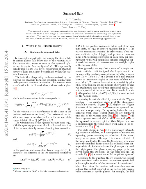
Squeezed lightA. I. LvovskyInstitute for Quantum Information Science, University of Calgary, Calgary, Canada, T2N 1N4 and Russian Quantum Center, 100 Novaya St., Skolkovo, Moscow region, 143025, Russia∗ (Dated: January 17, 2014) The squeezed state of the electromagnetic field can be generated in many nonlinear optical processes and finds a wide range of applications in quantum information processing and quantum metrology. This article reviews the basic properties of single-and dual-mode squeezed light states, methods of their preparation and detection, as well as their quantum technology applications.I.WHAT IS SQUEEZED LIGHT? A. Single-mode squeezed lightIn squeezed states of light, the noise of the electric field at certain phases falls below that of the vacuum state. This means that, when we turn on the squeezed light, we see less noise than no light at all. This apparently paradoxical feature is a direct consequence of quantum nature of light and cannot be explained within the classical framework. The basic idea of squeezing can be understood by considering the quantum harmonic oscillator, familiar from undergraduate quantum mechanics. Its vacuum state wavefunction in the dimensionless position basis is given by1 1 −X 2 /2 e , π 1/4 which in the momentum basis corresponds to ψ0 (X ) = ˜0 (P ) = √1 ψ 2π+∞(1)e−iP X ψ0 (X )dX =−∞1 π 1 /4e −P2/2(2) (so the vacuum state wavefunction is the same in the position and momentum bases). The variance of the position and momentum observables in the vacuum state equals 0| ∆X 2 |0 = 0| ∆P 2 |0 = 1/2. The wavefunction of the squeezed-vacuum state |sqR with the squeezing parameter R > 0 is obtained from that of the vacuum state by means of scaling transformation: √ 2 R ψR (X ) = 1/4 e−(RX ) /2 , (3) π and 2 1 ˜R (P ) = √ e−(P/R) /2 ψ (4) 1 / 4 π R in the position and momentum bases, respectively. In this state, the variances of the two canonical observables are ∆X 2 = 1/(2R2 ) and ∆P 2 = R2 /2. (5)∗ 1lvov@ucalgary.ca ˆ P ˆ ] = i for the quadrature observables. We use convention [X,If R > 1, the position variance is below that of the vacuum state, so |sqR is position-squeezed ; for R < 1 the state is momentum-squeezed. In other words, if we prepare multiple copies of |sqR , and perform a measurement of the squeezed observable on each copy, our measurement results will exhibit less variance than if we performed the same set of measurements on multiple copies of the vacuum state. More generally, we say that a state of a single harmonic oscillator exhibits (quadrature) squeezing if the variance of the position, momentum, or any other quadraˆθ = X ˆ cos θ + P ˆ sin θ (where θ is a real number ture X known as quadrature angle ) in that state exhibits variance below 1/2. In accordance with the uncertainty principle, both position and momentum observables, or any two quadratures associated with orthogonal angles, cannot be squeezed at the same time. For example, in state (1) the product ∆X 2 ∆P 2 = 1/4 is the same as that for the vacuum state. Squeezing is best visualized by means of the Wigner function — the quantum analogue of the phase-space probability density. Figure 1(c,d) display the Wigner functions of the position- and momentum-squeezed vacuum states, respectively. The squeezing feature becomes apparent when these Wigner functions are compared with that of the vacuum state [Fig. 1(a)]. Figure 1(e,f) shows squeezed coherent states, which are analogous to the squeezed vacuum except that their Wigner function is displaced from the phase space origin akin to the coherent state [Fig. 1(b)]. The state shown in Fig. 1(f) is particularly interesting because it exhibits, as a consequence of momentum squeezing, phase squeezing — reduction of the uncertainty in the phase with respect to a coherent state of the same amplitude. Because the Schr¨ odinger evolution under the standard harmonic oscillator Hamiltonian corresponds to clockwise rotation of the phase space around the origin point, the phase squeezing property is preserved under this evolution. In the same context, the state in Fig. 1(e) is sometimes called amplitude squeezed. According to the quantum theory of light, the Hilbert space associated with a mode of the electromagnetic field is isomorphic to that of the mechanical harmonic oscillator. The role of the position and momentum observables in this context is played by the electric field magnitudes measured at specific phases. For example, the fieldarXiv:1401.4118v1 [quant-ph] 15 Jan 20142 at phase zero (with respect to a certain reference) corresponds to the position observable, that at phase π/2 to the momentum observable, and so on. Accordingly, phase-sensitive measurements of the field in an electromagnetic wave are affected by quantum uncertainties. For the coherent and vacuum states, this uncertainty is ω/2ε0 V (the standard phase-independent and equals quantum limit, or SQL), where ω is the optical frequency and V is the quantization volume [1]. But squeezed optical states exhibit uncertainties below SQL at certain phases. Dependent on whether the mean coherent amplitude of the state is zero, squeezed optical states are classified into squeezed vacuum and (bright) squeezed light. Squeezed coherent states form a subset of bright squeezed light states. zero while its variance equals ∆X 2 = ψ | (ˆ a+a ˆ † )2 1 |ψ = − s, 2 2 (7)so for state |ψ is position squeezed for positive s.a)pump crystalb)pump photon pair crystal photon pairFIG. 2. Spontaneous parametric down-conversion. a) Degenerate configuration, leading to single-mode squeezed vacuum. b) Non-degenerate configuration, leading to two-mode squeezed vacuum.a)2 -2 -2b)P-2 0 2 4 6X-2 0 2P2 -2 -2P-2 0 2 4 6X-2 0 2P246XDj 246Xc)2 -2 -2d)P-2 0 2 4 6X6-2 0 2P-22P-2 0 2 4 6X6-2 0 2P24X2 -24Xe)2 -2 -2f)P-2 0 2 4 6X6-2 0 2P-22P24X-2 0 2 4 6 -2 0 2 Dj X 2 4 6XP-2FIG. 1. Wigner functions of certain single-oscillator states. a) Vacuum state. b) coherent state. c,d) Position- and momentum-squeezed vacuum states. e,f) Position- and momentum-squeezed coherent states with real amplitudes. Panels (b) and (f) show the phase uncertainties of the respective states to emphasize the phase squeezing of state (f). Insets show wavefunctions in the position and momentum bases.This result illustrates one of the primary methods of producing squeezing. Spontaneous parametric downconversion (SPDC) is a nonlinear optical process in which a photon of a powerful laser field propagating through a second-order nonlinear optical medium may split into two photons of lower energy. The frequencies, wavevectors and polarizations of the generated photons are governed by phase-matching conditions. Single-mode squeezing, such as that in the above example, is obtained when SPDC is degenerate : the two generated photons are indistinguishable in all their parameters: frequency, direction, and polarization. The quantum state of the optical mode into which the photon pairs are emitted exhibits squeezing [Fig. 2(a)]. Aside from being an interesting physical entity by itself, squeezed light has a variety of applications. One of the primary applications of single-mode squeezed light is in precision measurements of distances. Such measurements are typically done by means of interferometry. Quantum phase noise poses an ultimate limit to interferometry, and the application of squeezing (in particular, the phase squeezed state discussed above) permits expanding this limit beyond a fundamental boundary. For example, squeezing is employed in the new generation of gravitational wave detectors — GEO 600 in Europe and LIGO in the United States.B. Two-mode squeezed lightHow can one generate optical squeezed states in experiment? Consider the state s |ψ = |0 − √ |2 , 2 (6)where |0 and |2 are photon number (Fock) states and s is a real positive number. We assume s to be small, so the norm of state (6) is close to one. √ The mean value of ˆ = (ˆ the position operator X a+a ˆ† )/ 2 in this state isA state that is closely related to the single-oscillator squeezed vacuum in its theoretical description and experimental procedures, but quite different in properties is the two-mode squeezed vacuum (TMSV), also known as the twin-beam state. As the name suggests, this is a state of not one, but two mechanical or electromagnetic oscillators. We introduce this state by first analyzing the tensor product |0 ⊗ |0 of vacuum states of the two oscillators. In the position basis, its wavefunction [Fig. 3(a)],2 2 1 Ψ00 (Xa , Xb ) = √ e−Xa /2 e−Xb /2 π(8)3 can be rewritten as2 2 1 Ψ00 (Xa , Xb ) = √ e−(Xa −Xb ) /4 e−(Xa +Xb ) /4 . πboth Alice’s and Bob’s observables: (9) 1 −(Pa −Pb )2 /(4R2 ) −R2 (Pa +Pb )2 /4 ˜ R (Pa , Pb ) = √ Ψ e e . (11) π We see that for R > 1 Alice’s and Bob’s momenta are √ anticorrelated, i.e. the variance of the sum (Pa + Pb )/ 2 is below the level expected from two vacuum states [Fig. 3(d)]. The two-mode squeezed vacuum does not imply squeezing in each individual mode. On the contrary, Alice’s and Bob’s position and momentum observables in TMSV obey a Gaussian probability distribution with variance2 2 2 2 ∆Xa = ∆Xb = ∆ Pa = ∆ Pb =Here, Xa and Xb are the position observables of the two oscillators which are traditionally associated with fictional experimentalists Alice and Bob. The meaning √ of Eq. (9) √ is that the observables (Xa − Xb )/ 2 and (Xa + Xb )/ 2 have a Gaussian distribution with variance 1/2. This is not surprising because in the double-vacuum state Alice’s and Bob’s position observables are uncorrelated and both of them have variance 1/2. The behavior of the momentum quadratures in this state is analogous to that of the position.a)4 2 -4 -2 -2 -4XB4 2 2 4PB1 + R4 . 4R2(12)XA-4-2 -2 -424PAthat exceeds that of the vacuum state for any R = 1. In other words, each mode of a TMSV considered individually is in the thermal state. With increasing R > 1, the uncertainty of individual quadratures increases while that of the difference of Alice’s and Bob’s position observables as well as the sum of their momentum observables decreases. In the extreme case of R → ∞, the wavefunctions of the two-modes squeezed state take the form ΨR (Xa , Xb ) ∝ δ (Xa − Xb ) ˜ R (Pa , Pb ) ∝ δ (Pa + Pb ) Ψ (13) (14)b)4 2 -4 -2 -2 -4XB4 2 2 4PBXA-4-2 -2 -424PAFIG. 3. Wavefunctions (not Wigner functions!) of two-mode states in the position (left) and momentum (right) bases. a) Double-vacuum state is uncorrelated in both bases. b) The two-mode squeezed state with position observables correlated, and momentum observables anticorrelated beyond the standard quantum limit.The wavefunction of the two-mode squeezed vacuum state |TMSVR is given by2 2 2 2 1 ΨR (Xa , Xb ) = √ e−(Xa +Xb ) /(4R ) e−R (Xa −Xb ) /4 , π (10) where R, as previously, is the squeezing parameter [Fig. 3(c)]. In contrast to the double-vacuum, TMSV is an entangled state, and Alice’s and Bob’s position observables are nonclassically correlated thanks to that √ entanglement. For R > 1, the variance of (Xa − Xb )/ 2 is less than 1/2, i.e. below the value for the double vacuum state. The wavefunction of TMSV in the momentum basis is obtained from Eq. (10) by means of Fourier transform byBoth Alice’s and Bob’s positions are completely uncertain, but at the same time precisely equal, whereas the momenta are precisely opposite. This state is the basis of the famous quantum nonlocality paradox in its original formulation of Einstein, Podolsky and Rosen (EPR) [2]. EPR argued that by choosing to perform either a position or momentum measurement on her portion of the TMSV, Alice remotely prepares either a state with a certain position or one with a certain momentum at Bob’s location. But according to the uncertainty principle, certainty of position implies complete uncertainty of momentum, and vice versa. In other words, by choosing the setting of her measurement apparatus, Alice can instantly and remotely, without any interaction, prepare at Bob’s station one of two mutually incompatible physical realities. This apparent contradiction to basic principles of causality has lead EPR to challenge quantum mechanics as complete description of physical reality and triggered a debate that continues to this day. Experimental realization of TMSV is largely similar to that of single-mode squeezing. SPDC is the primary method; however, in contrast to the single-mode case, it is implemented in the non-degenerate configuration. The photons is each generated pair are emitted into two distinguishable modes that become carriers of the TMSV state [Fig. 2(b)]. In order to understand how non-degenerate SPDC leads to squeezing, consider the two-mode state |Ψ = |0 ⊗ |0 + s |1 ⊗ |1 , (15)4 i.e. a pair of photons has been emitted into Alice’s and Bob’s modes with amplitude s. Now √ if we evaluate the variance of the observable (Xa − Xb )/ 2, we find 1 1 1 ∆(Xa − Xb )2 = Ψ| (ˆ a+a ˆ† − ˆ b−ˆ b† )2 |Ψ = − s, 2 4 2 (16) i.e. Alice’s and Bob’s position observables are correlated akin to TMSV. A similar calculation shows anticorrelation of Alice’s and Bob’s momentum observables. Both the single-mode and two-mode squeezed vacuum states are valuable resources in quantum optical information technology. TMSV, in particular, is useful for generating heralded single photons and unconditional quantum teleportation.II. SALIENT FEATURES OF SQUEEZED STATES A. The squeezing operatorIf this evolution continues for time t, we will have ˆ (t) = S ˆ † (r )X ˆ (0)S ˆ (r ) = X ˆ (0)e−r ; X ˆ (t) = S ˆ † (r )P ˆ (0)S ˆ(r) = P ˆ (0)er , P (24a) (24b)which corresponds to position squeezing by factor R = er and corresponding momentum antisqueezing (Fig. 4). If the initial state is vacuum, the evolution will result in a squeezed vacuum state; coherent states will yield squeezed light [3]. As a self-check, we find the factor of quadrature squeezing in state (18), in analogy to Eq. (7): R= 0|∆X 2 |0 = ˆ† (r)∆X 2 S ˆ(r)|0 0|S 1/2 ≈1+r 1/2 − rwhich is in agreement with R = er for small r. The corresponding transformation of the creation and annihilation operators is given by a ˆ(t) = a ˆ(0) cosh r − a ˆ† (0) sinh r; a ˆ† (t) = a ˆ† (0) cosh r − a ˆ(0) sinh r, known as Bogoliubov transformation. (25a) (25b)We now proceed to a more rigorous mathematical description of squeezing. Single-mode squeezing occurs under the action of operator ˆ(ζ ) = exp[(ζ a S ˆ2 − ζ ∗ a ˆ†2 )/2], (17)Pwhere ζ = reiφ is the squeezing parameter, with r and φ being real numbers, upon the vacuum state. Phase φ determines the angle of the quadrature that is being squeezed. In the following, we assume this phase to be zero so ζ = r. Note that, for a small r, the squeezing operator (17) acting on the vacuum state, generates state √ ˆ(r) |0 ≈ [1+(ra S ˆ2 −r a ˆ†2 )/2] |0 = |0 −(r/ 2) |2 , (18) which is consistent with Eq. (6) for s = r. The action of the squeezing operator can be analyzed as fictitious evolution under Hamiltonian ˆ = i α[ˆ H a2 − (ˆ a† )2 ]/2 (19)Xˆ )t ˆ(r) = e−i(H/ for time t = r/α (so that S ). Analyzing this evolution in the Heisenberg picture, we use [ˆ a, a ˆ† ] = 1 to find that˙ = i [H, ˆ a a ˆ ˆ] = −αa ˆ† and ˙ † = −αa a ˆ ˆ.(20)FIG. 4. Transformation of quadratures under the action of the squeezing Hamiltonian (19) with α > 0. Grey areas show examples of Wigner function transformations with r = αt = ln 2.(21)Now using the expressions for quadrature observables √ √ ˆ = (ˆ ˆ = (ˆ X a+a ˆ† )/ 2 and P a−a ˆ† )/ 2i, (22) we rewrite Eqs. (20) and (21) as ˙ ˆ X = −αX ; ˙ ˆ P = αP. (23a) (23b)Two-mode squeezing is treated similarly. The twomode squeezing operator is ˆ2 (ζ ) = exp[(−ζ a S ˆˆ b + ζ ∗a ˆ†ˆ b† )]. (26)Assuming, again, a real ζ = r, introducing the fictitious Hamiltonian and recalling that the creation and annihilation operators associated with different modes commute,5 we find a ˆ(t) = a ˆ(0) cosh r + ˆ b(0)† sinh r; ˆ b(t) = ˆ b(0) cosh r + a ˆ(0)† sinh r; and hence ˆ a (t) ± X ˆ b (t) = [X ˆ a (0) ± X ˆ b (0)]e±r ; X ˆa (t) ± P ˆb (t) = [P ˆa (0) ± P ˆb (0)]e∓r . P (28a) (28b) (27a) (27b) Decomposing the exponent in right-hand side of the above equation into the Taylor series with respect to α, we obtain α 2m . m! n=0 m=0 (33) Because this equality must hold for any real α, each term of the sum in the left-hand side must equal its counterpart in the right-hand side that contains the same power of α. Hence n = 2m and 2R 1 + R2 2m |sqR = 1 − R2 2R 1 + R2 2(1 + R2 )m ∞αn n |sqR √ = n!∞1 − R2 2(1 + R2 )mInitially, Alice’s and Bob’s modes are in vacuum states, and the quadrature observables in these modes are uncorrelated. But as the time progresses, Alice’s and Bob’s position observables become correlated while the momentum observables become anticorrelated.(2m)! . m!(34)Since R = er , we haveB. Photon number statistics1 2R = 1 + R2 cosh rand1 − R2 = − tanh r, 1 + R2(35)An important component in the theoretical description of squeezed light is its decomposition in the photon number basis, i.e. calculating the quantities n |sqR for the single-mode squeezed state and mn |TMSVR for the two-mode state. Due to non-commutativity of the photon creation and annihilation operators, this calculation turns out surprisingly difficult even for basic squeezed vacuum states, let alone squeezed coherent states and the states that have been affected by losses. Possible approaches to this calculation include the disentangling theorem for SU(1,1) Lie algebra [4], direct calculation of the wavefunction overlap in the position space [5] or transformation of the squeezing operator [6]. Here we derive the photon number statistics of single- and twomode squeezed vacuum states by calculating their inner product with coherent states. The wavefunction of a coherent state with real amplitude α is ψα (X ) = 1 π 1/4 e−(X −α√ 2)2 /2so Eq. (34) can be rewritten as |sqR = √ 1 cosh r∞(− tanh r)mm=0(2m)! |2m . 2m m!(36)We stop here for a brief discussion. First, we note that that for r 1, Eq. (36) becomes √ |sqR = |0 − (r/ 2) |2 + O(r2 ), (37),(29)so its inner product with the position squeezed state (3) equalsR2 2R − 1+ α2 R2 . e 2 1+R −∞ (30) Now we recall that the coherent state is decomposed into the Fock basis according to+∞α |sqR =ψα (X )ψR (X )dX =∞|α =n=0e −α2/2αn √ |n , n!(31)consistently with Eq. (18). Second, note that the squeezed vacuum state (36) contains only terms with even photon numbers. This is a fundamental feature of this state; in fact, one of the earlier names for squeezed states has been “two-photon coherent states” [7]. This feature follows from the nature of the squeezing operator (17): in its decomposition into the Taylor series with respect to r, creation and annihilation operators occur only in pairs. Pairwise emission of photons is also a part of the physical nature of SPDC: due to energy conservation a pump photon can only split into two photons of half its energy. We now turn to finding the photon number decomposition of the two-mode squeezed state. We first notice, by looking at Eq. (26), that |RAB must only contain terms with equal photon numbers in Alice’s and Bob’s modes. This circumstance allows us to significantly simplify the algebra. We proceed along the same route as outlined above, calculating the overlap of |RAB with the tensor product |αα of identical coherent states |α in Alice’s and Bob’s channels using Eqs. (10) and (29): αα|TMSVR+∞so we have∞= α n |sqR √ = n!nψα (Xa )ψα (Xb )ΨR (Xa , Xb )dXa dXb−∞n=02R e 1 + R21−R2 α2 2(1+R2 )(32)=2R − 1+2R2 α2 e . 1 + R2(38)6 Decomposing the coherent states in the left-hand side into the Fock basis according to Eq. (31) and keeping only the terms with equal photon numbers, we have∞−R2 2 2R − 1 α2n α e 1+R2 nn| TMSVR √ = 2 1+R n!(39)n=0Now writing the Taylor series for the right-rand side and using Eq. (35), we obtain |TMSVR = 1 tanhn r |nn . cosh r n=0∞(40)FIG. 5. Experimentally reconstructed photon number statistics of the squeezed vacuum state. For low photon numbers, the even terms are greater than the odd terms due to pairwise production of photons, albeit the odd term contribution is nonzero due to loss. Reproduced from Ref. [10].position-squeezed vacuum ˆ¢(t ) bˆ¢(t ) a momentum-squeezed vacuumSimilarly to the single-mode squeezing, it is easy to verify that result is consistent with state (15) for small r. On the other hand, in contrast to the single-mode case, the energy spectrum of TMSV follows Boltzmann distribution with mean photon number in each mode n = sinh2 r. This is in agreement with our earlier observation that Alice’s and Bob’s portions of TMSV considered independently of their counterpart are in the thermal state, i.e. the state whose photon number distribution obeys Boltzmann statistics with the temperature given by e− ω/kT = tanh r. While the present analysis is limited to pure squeezed vacuum states, photon number decompositions of squeezed coherent states and squeezed states that have undergone losses can be found in the literature [8, 9]. In contrast to pure squeezed vacuum states, these decompositions have nonzero terms associated to non-paired photons. The origin of these terms is easily understood. If a one- or two-mode squeezed vacuum state experiences a loss, it may happen that one of the photons in a pair is lost while the other one remains. If the squeezing operator acts on a coherent state, the odd photon number terms will appear in the resulting state because they are present initially. Photon statistics of both classes of squeezed states have been tested experimentally, as discussed in Section III below. An example is shown in Fig. 5.ˆ0 a fictitious input vacuum ˆ0 bˆ(0) b input vacuum2-mode squeezerˆ(0) aˆ(t ) a two-mode squeezed vacuum ˆ(t ) bFIG. 6. Interconversion of the two-mode squeezed vacuum and two single-mode squeezed vacuum states. Dashed lines show a fictitious beam splitter transformation of a pair of vacuum states such that the modes a ˆ (t), ˆ b (t) are explicitly single-mode squeezed with respect to modes a ˆ 0, ˆ b 0.In accordance with the definition (22) of quadrature observables, Eqs. (41) apply in the same way to the position and momentum of the input and output modes. Applying this to Eqs. (28), we find √ ˆ a,b = [X ˆ a (t) ∓ X ˆ b (t)]/ 2 X √ ˆ a (0) ∓ X ˆ b (0)]/ 2 = e ∓r [ X (42) for the output positions and √ ˆa,b = [P ˆa (t) ∓ P ˆb (t)]/ 2 P √ ˆa (0) ∓ P ˆb (0)]/ 2 = e ±r [ PC.Interconversion between single- and two-mode squeezing(43)If the modes of the TMSV are overlapped on a symmetric beam splitter, two unentangled single-mode vacuum states will emerge in the output (Fig. 6). To see this, we recall the beam splitter transformation a ˆ = τa ˆ − ρˆ b; ˆ ˆ b = τ b + ρa ˆ, (41a) (41b)for the momenta. In order to understand what state this corresponds to, let us assume, for the sake of the argument, that vacuum modes a ˆ and ˆ b at the SPDC input have been obtained from another pair of modes by means of another symmetric beam splitter: √ a ˆ0 = [ˆ a(0) − ˆ b(0)]/ 2 (44) √ 0 ˆ ˆ b = [ˆ a(0) + b(0)]/ 2. (45) Of course, since modes a ˆ(0) and ˆ b(0) are in the vacuum 0 0 ˆ state, so are a ˆ and b . We then have:0 ˆ a,b = e∓r X ˆ a,b X ; ±r ˆ 0 ˆ Pa,b = e Pa,b ,where τ and ρ are the beam splitter amplitude transmissivity and reflectivity, respectively. For a symmetric √ beam splitter, τ = ρ = 1/ 2. In writing Eqs. (41), we neglected possible phase shifts that may be applied to individual input and output modes [5].(46)7 where superscript 0 associates the quadrature with modes a ˆ0 and ˆ b0 . We see that modes a ˆ and ˆ b are re0 0 ˆ lated to vacuum modes a ˆ and b by means of position and momentum squeezing transformations, respectively. Because the beam-splitter transformation is reversible, it can also be used to obtain a TMSV from two singlemode squeezed vacuum states with squeezing in orthogonal quadratures. This technique has been used, for example, in the experiment on continuous-variable quantum teleportation [11].E. Effect of lossesD.Squeezed vacuum and squeezed lightSqueezed vacuum and bright squeezed light are readily converted between each other by means of the phasespace displacement operator [5], whose action in the Heisenberg picture can be written as ˆ † (α)ˆ ˆ (α) = a D a† D ˆ + α. (47)Squeezed states that occur in practical experiments necessarily suffer from losses present in sources, transmission channels and detectors. In order to understand the effect of propagation losses on a single-mode squeezed vacuum state, we can use the model in which a lossy optical element with transmission T is replaced by a beam splitter (Fig. 8). At the other input port of the beam splitter there is a vacuum state. The interference of the signal mode a ˆ with the vacuum mode v ˆ will produce a mode with operator a ˆ = τa ˆ − ρv ˆ (with τ 2 = T and ρ2 = 1 − T being the beam splitter transmissivity and reflectivity) in the beam splitter output. Accordingly, we have ˆ θ,out = τ X ˆ a,θ − ρX ˆ v,θ . X (52)This means, in particular, that the position and momentum transform according to √ ˆ →X ˆ + Re α 2; (48) X √ ˆ ˆ P → P + Im α 2, (49) ˆ (α), the entire phase space disso, under the action of D places itself, thereby changing the coherent amplitude of the squeezed state without changing the degree of squeezing.Because the quadrature observable of the signal and vacuum states are uncorrelated, and since ∆(Xθ )2 = 1/2, it follows that2 2 ∆Xθ, ∆(Xa,θ )2 + ρ2 ∆(Xv,θ )2 out = τ= T ∆(Xa,θ )2 + (1 − T )/2.(53)Analyzing Eqs. (41) we see that the optical loss alone, no matter how significant, cannot eliminate the property of squeezing completely.ˆ alow-reflectivity beam splitterˆ - rb aˆ aˆ b b1signalˆout aoutputFIG. 7. Implementation of phase-space displacement. ρ is the beam splitter’s amplitude reflectivity.ˆ vacuum vFIG. 8. The beam splitter model of loss.Phase-space displacement can be implemented experimentally by overlapping the signal state with a strong coherent state |β on a low-reflectivity beam splitter (Fig. 7). Applying the beam splitter transformation (41), we find for the signal mode a ˆ = τa ˆ − ρˆ b (50)Given that mode ˆ b is in a coherent state (i.e. an eignestate of ˆ b) and that ρ 1 (i.e. τ ∼ 1), we have a ˆ =a ˆ − ρβ (51)in analogy to Eq. (47). The displacement operation has been used to change the amplitude of squeezed light in many experiments, for example, in Ref. [12].Ideal squeezed-vacuum and coherent states have the minimum-uncertainty property: the product of uncer2 2 tainties ∆Xout ∆Pout reaches the theoretical minimum of 1/4. But this is no longer the case in the presence of losses. The deviation of the uncertainty from the minimum can be used to estimate the preparation quality of a squeezed state. Suppose a measurement of a squeezed state yielded the minimum and maximum quadrature un2 2 and ∆Xmax , respectively. certainty values of ∆Xmin One can assume that the state has been obtained from an ideal (minimum-uncertainty) squeezed state with squeezing R by means of loss channel with transmissivity T . Using Eq. (5) and solving Eqs. (53), one finds T [13], which can then be compared with the values expected from the setup at hand.。
动态对等的最佳策略
Electric Power Systems Research 84 (2012) 58–64Contents lists available at SciVerse ScienceDirectElectric Power SystemsResearchj o u r n a l h o m e p a g e :w w w.e l s e v i e r.c o m /l o c a t e /e p srDynamic equivalence by an optimal strategyJuan M.Ramirez a ,∗,Blanca V.Hernández a ,Rosa Elvira Correa b ,1a Centro de Investigación y de Estudios Avanzados del I.P.N.,Av del Bosque 1145.Col El Bajio,Zapopan,Jal.,45019,MexicobUniversidad Nacional de Colombia –Sede Medellín.Facultad de Minas.Carrera 80#65-223Bloque M8,114,Medellín,Colombiaa r t i c l ei n f oArticle history:Received 21May 2011Received in revised form 26September 2011Accepted 29September 2011Keywords:Power system dynamics Equivalent circuitPhasor measurement unit Stability analysisPower system stabilitya b s t r a c tDue to the curse of dimensionality,dynamic equivalence remains a computational tool that helps to analyze large amount of power systems’information.In this paper,a robust dynamic equivalence is proposed to reduce the computational burden and time consuming that the transient stability studies of large power systems represent.The technique is based on a multi-objective optimal formulation solved by a genetic algorithm.A simplification of the Mexican interconnected power system is tested.An index is used to assess the proximity between simulations carried out using the full and the reduced model.Likewise,it is assumed the use of information stemming from power measurements units (PMUs),which gives certainty to such information,and gives rise to better estimates.© 2011 Elsevier B.V. All rights reserved.1.IntroductionOne way to speed up the dynamic studies of currently inter-connected power systems without significant loss of accuracy is to reduce the size of the system model by means of dynamic equiva-lents.The dynamic equivalent is a simplified dynamic model used to replace an uninterested part,known as an external part,of a power system model.This replacement aims to reduce the dimension of the original model while the part of interest remains unchanged [1–6].The phrases “Internal system”(IS)and “external system”(ES)are used in this paper to describe the area in question,and the remaining regions,respectively.Boundary buses and tie lines can be defined in each IS or ES.It is usually intended to perform detailed studies in the IS.However,the ES is important to the extent where it affects IS analyses.The equivalent does not alter the transient behavior of the part of the system that is of concern and greatly reduces the dimen-sion of the network,reducing computational time and effort [4,7,8].The dynamic equivalent also can meet the accuracy in engineering,achieving effective,rapid and precise stability analysis and security controls for large-scale power system [4,8].However,the determi-∗Corresponding author.Tel.:+523337773600.E-mail addresses:jramirez@gdl.cinvestav.mx (J.M.Ramirez),bhernande@gdl.cinvestav.mx (B.V.Hernández),elvira.correa@ (R.E.Correa).1Tel.:+57314255140.nation of dynamic equivalents may also be a time consuming task,even if performed off-line.Moreover,several dynamic equivalents may be required to represent different operating conditions of the same system.Therefore,it is important to have computational tools that automate the procedure to evaluate the dynamic equivalent [7].Ordinarily,dynamic equivalents can be constructed follow-ing two distinct approaches:(i)reduction approach,and (ii)identification approach.The reduction approach is based on an elimination/aggregation of some components of the existing model [4,5,9].The two mostly found in the literature are known as modal reduction [6,10]and coherency based aggregation [2,11,12].The identification approach is based on either parametric or non-parametric identification [13,14].In this approach,the dynamic equivalent is determined from online measurements by adjusting an assumed model until its response matches with measurements.Concerning the capability of the model,the dynamic equivalent obtained from the reduction approach is considerably more reli-able and accurate than those set up by the identification approach,because it is determined from an exact model rather than an approximation based on measurements.However,the reduction-based equivalent requires a complete set of modeling data (e.g.model,parameters,and operating status)which is rarely avail-able in practice,in particular the generators’dynamic parameters [5,13,15,16].On the other hand,due to the lack of complete system data,and/or frequently variations of the parameters with time,the importance of estimation methods is revealed noticeably.Especially,on-line model correction aids for employing adaptive0378-7796/$–see front matter © 2011 Elsevier B.V. All rights reserved.doi:10.1016/j.epsr.2011.09.023J.M.Ramirez et al./Electric Power Systems Research84 (2012) 58–6459Fig.1.190-buses46-generators power system.controllers,power system stabilizers(PSS)or transient stability assessment.The capability of such methods has become serious rival of the old conventional methods(e.g.the coherency[11,12] and the modal[6,10]approaches).The equivalent estimation meth-ods have spread,because it can be estimated founded on data measured only on the boundary nodes between the study system and the external system.This way,without any need of informa-tion from the external system,estimation process tries to estimate a reduced order linear model,which is replaced for the external part.Evidently,estimation methods can be used,in presence of perfect data of the network as well to compute the equivalent by simulation and/or model order reduction[15].Sophisticated techniques have become interesting subject for researchers to solve identification problems since90s.For example, to obtain a dynamic equivalent of an external subsystem,an opti-mization problem has been solved by the Levenberg–Marquardt algorithm[17].Artificial neural networks(ANN)are the most prevalent method between these techniques because of its high inherent ability for modeling nonlinear systems,including power system dynamic equivalents[15,18–25].Power system real time control for security and stability has pro-moted the study of on-line dynamic equivalent technologies,which progresses in two directions.One is to improve the original off-line method.The mainstream approach is to obtain equivalent model based on typical operation modes and adjust equivalent parame-ters according to real time collected information[4].Distributed coordinate calculation based on real time information exchanging makes it possible to realize on-line equivalence of multi-area inter-connected power system in power market environment[4].Ourari et al.[26]developed the slow coherency theory based on the struc-ture preservation technique,and integrated dynamic equivalence into power system simulator Hypersim,verifying the feasibility of on-line computation from both computing time and accuracy[27].Prospects of phasor measurement technique based on global positioning system(GPS)applied in transient stability control of power system are introduced in Ref.[4].Using real data collected by phasor measurement unit(PMU),with the aid of GPS and high-speed communication network,online dynamic equivalent of interconnected power grid may be achieved[4].In this paper,the dynamic equivalence problem is formulated by two objective functions.An evolutionary optimization method based on genetic algorithms is used to solve the problem.2.PropositionThe main objective of this paper is the external system’s model order reduction of an electrical grid,preserving only the frontier nodes.That is,those nodes of the external system directly linked to nodes of the study system.At such frontier nodes,fictitious gen-erators are allocated.The external boundary is defined by the user. Basically,it is composed by a set of buses,which connect the exter-nal areas to the study system.There is not restriction about this set. Different operating conditions are taken into account.work reductionAfirst condition for an equivalence strategy is the steady state preservation on the reduced grid;this means basically a precise60J.M.Ramirez et al./Electric Power Systems Research 84 (2012) 58–64Fig.2.Proposed strategy’s flowchart.voltage calculation.In this paper,all nodes of the external system are eliminated,except the frontier nodes.By a load flow study,the complex power that should inject some fictitious generators at such nodes can be calculated.The nodal balance equation yields,j ∈Jp ij +Pg i +Pl i =0,∀i ∈I(1)where I is the set of frontier nodes;J is the set of nodes linked directly to the i th frontier node;p ij is the active power flowing from the i th to j th node;Pg i is the generation at the i th node;Pl i is the load at the i th node.Thus,the voltages for the reduced model become equal to those of the full one.For studies where unbalanced conditions are important,a similar procedure could be followed for the negative and zero equivalent sequences calculation.2.2.Studied systemThe power system shown in Fig.1depicts a reduced version of the Mexican interconnected power system.It encompasses 7regional systems,with a generation capacity of 54GW in 2004and an annual consumption level of 183.3TWh in 2005.The transmis-sion grid comprises a large 400/230kV system stretching from the southern border with Central America to its northern interconnec-tions with the US.The grids at the north and south of the country are long and sparsely interconnected transmission paths.The major load centers are concentrated on large metropolitan areas,mainly Mexico City in the central system,Guadalajara City in the western system,and Monterrey City in the northeastern system.The subsystem on the right of the dotted line is considered as the system under study.Thus,the subsystem on the left is the exter-nal one.There are five frontier nodes (86,140,142,148and 188)and six frontier lines (86–184,140–141,142–143,148–143(2)and 188–187).Thus,the equivalent electrical grid has five fictitious generators at nodes 86,140,142,148and 188.Transient stabil-ity models are employed for generators,equipped with a static excitation system;its formulation is described as follows,dıdt=ω−ω0(2)dωdt=1T j [Tm −Te −D (ω−ω0)](3)dE q dt=1T d 0 −E g −(x d −x d )i d +E fd(4)dE ddt =1T d 0−E d +(x q −xq )i q (5)dE fd dt=1T A−E fd +K A (V ref +V s −|V t |) (6)where ı(rad)and ω(rad/s)represent the rotor angular positionand angular velocity;E d (pu)and E q(pu)are the internal transient voltages of the synchronous generator;E fd (pu)is the excitationvoltage;i d (pu)and i q (pu)are the d -and q -axis currents;T d 0(s)and T q 0(s)are the d -and q -open-circuit transient time constants;x’d (pu)and x q(pu)are the d -and q -transient reactances;Tm (pu)and Te (pu)are the mechanical and electromagnetic nominal torque;Tj is the moment of inertia;D is the damping factor;K A and T A (s)are the system excitation gain and time constant;V ref is the voltage reference;V t is the terminal voltage;V s is the PSS’s output (if installed).The corresponding parameters are selected as typical [28].2.3.FormulationGiven some steady state operating point (#CASES )the following objective functions are defined,min f =[f 1f 2]f 1=#CASESop =1w 1opNg intk =1ωk ori (t )−ωkequiv (x,t )2(7)f 2=#CASESop =1w 2opNg intk =1Pe kori (t )−Pe k equiv (x,t )2(8)subject to:0=Ngen eqj =1H j −ni =1i ∈LH i(9)where ωk ori is the time behavior of the angular velocity of those generators in the original system,that will be preserved (Ng int),J.M.Ramirez et al./Electric Power Systems Research84 (2012) 58–6461Fig.3.Fitness assignment of NSGA-II in the two-objective space.Fig.4.Case1:from top to bottom(i)angular position37(referred to slack);(ii)angular speed28;(iii)electrical torque41,after a three-phase fault at bus172.62J.M.Ramirez et al./Electric Power Systems Research 84 (2012) 58–64Fig.5.Case 3:from top to bottom (i)angular position 40(referred to slack);(ii)angular speed 34;(iii)electrical torque 39,after a three-phase fault at bus 144.after a disturbance within the internal area;ωk equiv is the time behavior of the angular velocity of those generators in the equiv-alent system,after the same disturbance within the internal area;Pe k ori is the time behavior of the electrical power of those gen-erators of the original system within the internal area;Pe k equiv is the time behavior of the electrical power of those generators in the equivalent system within the internal area;H k is the k th genera-tor’s inertia;L is the set of generators that belong to the external system;Ngen eq is the number of equivalent generators [16,25].The set of voltages S ={V i ,V j ,...,V k |complex voltages stemming from PMUs }has been included in the solution.The main challenge in a multi-objective optimization environ-ment is to minimize the distance of the generated solutions to the Pareto set and to maximize the diversity of the developed Pareto set.A good Pareto set may be obtained by appropriate guiding of the search process through careful design of reproduction oper-ators and fitness assignment strategies.To obtain diversification special care has to be taken in the selection process.Special care is also to be taken to prevent non-dominated solutions from being lost.Elitism addresses the problem of losing good solutions dur-ing the optimization process.In this paper,the NSGA-II algorithm (Non dominated Sorting Genetic Algorithm-II)[29–31]is used to solve the formulation.The algorithm NSGA-II has demonstrated to exhibit a well performance;it is reliable and easy to handle.It uses elitism and a crowded comparison operator that keeps diver-sity without specifying any additional parameters.Pragmatically,it is also an efficient algorithm that has shown better results to solve optimization problems with multi-objective functions in a series of benchmark problems [31,32].There are some other meth-ods that may be used.For instance,it is possible to use at least two population-based non-Pareto evolutionary algorithms (EA)and two Pareto-based EAs:the Vector Evaluated Genetic Algorithm (VEGA)[36],an EA incorporating weighted-sum aggregation [33],the Niched Pareto Genetic Algorithm [34,35],and the Nondom-inated Sorting Genetic Algorithm (NSGA)[29–31];all but VEGA use fitness sharing to maintain a population distributed along the Pareto-optimal front.3.ResultsIn this case,the decision variables,x ,are eight parametersper each equivalent generator:{x d ,x d ,x q ,x q ,T d 0,T q 0,H,D }.In this paper,for five equivalent generators,there are 40parameters to be estimated.Likewise,in this case,a random change in the load of all buses gives rise to the transient behavior.A normal distribution with zero mean is utilized to generate the increment (decrement)in all buses.The variation is limited to a maximum of 50%.The disturbance lasts for 0.12s and then it is eliminated;the studied time is 2.0s.To attain more precise equivalence for severe operating conditions,this improvement could require load variations greater than 50%.However,this bound was used in all cases.Fig.2depicts a flowchart of the followed strategy to calculate an optimal solution.In this paper,three operating points are taken into account:(i)Case 1,the nominal case [37];(ii)Case 2,an increment of 40%in load and generation;(iii)Case 3,a decrement of 30%in load and gen-eration.To account for each operating condition into the objective functions,the same weighted factors have been utilized (w i =1/3),Eqs.(7)–(8).Table 1summarizes the estimated parameters for five equiv-alent generators,according to the two objective functions.TheJ.M.Ramirez et al./Electric Power Systems Research84 (2012) 58–6463 Table1Parameters of the equivalent under a maximum of50%in load variation.G equiv1G equiv2G equiv3G equiv4G equiv5f1f2f1f2f1f2f1f2f1f2x d0.1080.104 2.140 2.100 1.920 1.9100.1590.1790.3240.362x d0.1130.1130.8190.8690.3960.3960.08760.132 1.900 1.950T d010.7010.7039.6039.6018.8018.7011.5011.5011.7011.70x q0.7100.7500.5300.5190.2880.308 2.470 2.4600.7050.803x q0.3950.3850.8740.8050.9010.9260.9220.9530.8820.884T q0 4.950 4.82033.3033.40 4.280 4.10016.9016.9012.8012.90H 4.610 4.61022.2722.2747.2647.2669.2369.2333.9333.93D18.0318.40535.6536.6239.2239.141.9042.00705.1705.2 electromechanical modes associated to generators of the internalsystem are closely preserved.These generators arefictitious andbasically are useful to preserve some of the main interarea modesbetween the internal area and the external one[16].Thus,in order to avoid the identification of the equivalent gener-ators’parameters based on a specific disturbance,in this paper theuse of random changes in all the load buses is used.This will giverise to parameters valid for different fault locations.The allowedchange in the load(in this paper,50%)will result in a slight varia-tion of transient reactances.Further studies are required to assesssensitivities.Fig.3shows a typical Pareto front for this application.The NSGA-II runs on a Matlab platform and the convergence lastsfor3.25h for a population of200individuals and20generations.It is assumed that phasor measurement units(PMUs)areinstalled at specific buses(188,140,142,148,and86in the externalsystem,and141,143,145,and182in the internal system),whichbasically correspond to the frontier nodes.Likewise,it is assumedthat the precise voltages are known in these buses every time.Bythe inclusion of the PMUs,there is a noticeable improvement in thevoltages’information at the buses near them,due to the fact that itis assumed the PMUs’high precision.In this paper,the simulation results obtained by the full andthe reduced system are compared by a closeness measure,themean squared error(MSE).The goal of a signalfidelity measureis to compare two signals by providing a quantitative score thatdescribes the degree of similarity/fidelity or,conversely,the levelof error/distortion between ually,it is assumed that oneof the signals is a pristine original,while the other is distorted orcontaminated by errors[38].Suppose that z={z i|i=1,2,...,N}and y={y i|i=1,2,...,N}aretwofinite-length,discrete signals,where N is the number of signalsamples and z i and y i are the values of the i th samples in z and y,respectively.The MSE is defined by,MSE(z,y)=1NNi=1(z i−y i)2(10)Figs.4–5illustrate the transient behavior of some representa-tive signals after a three-phase fault at buses172(Fig.4)for theCase1;and144(Fig.5)for the Case3.Bus39is selected as theslack bus.Values in Table2show the corresponding MSE valuesfor the twelve generators of the internal system for each operat-ing case.Such values indicate a close relationship between the fulland reduced signals’behavior.In order to improve the equivalenceof a specific operating point,it is possible to weight it differentlythrough the factors w1–3,Eqs.(7)–(8).Table2shows the MSE’s val-ues when Case2has a higher weighting than Case1and Case3(w2=2/3,w1=w3=1/6).These values indicate that a closer agree-ment is attained between signals with the full and the reducedmodel.It is emphasized that the equivalence’s improvement couldrequire load variations greater than50%for off-nominal operatingconditions.4.ConclusionsUndoubtedly,the power system equivalents’calculationremains a useful strategy to handle the large amount of data,cal-culations,information and time,which represent the transientstability studies of modern power grids.The proposed approachis founded on a multi-objective formulation,solved by a geneticalgorithm,where the objective functions weight independentlyeach operating condition taken into account.The use of informationstemming from PMUs helps to improve the estimated equivalentgenerators’parameters.Results indicate that the strategy is ableto closely preserve the oscillating modes associated to the inter-nal system’s generators,under different operating conditions.Thatis due to the preservation of the machines’inertia.The use ofan index to measure the proximity between the signal’s behav-ior after a three-phase fault,indicates that good agreement isattained.In this paper,the same weighting factors have been usedto assess different operating conditions into the objective func-tions.However,depending on requirements,these factors can bemodified.The equivalence based on an optimal formulation assuresTable2MSE for Case2(Three-Phase Fault at Bus168).Angular position Angular speed Electrical powerw k=1/3w2=2/3,w1=w3=1/6w k=1/3w2=2/3,w1=w3=1/6w k=1/3w2=2/3,w1=w3=1/6 Gen39 2.13E−01 1.54E−01 6.36E−05 6.90E−059.40E−02 6.91E−02Gen28 1.79E−019.39E−02 3.43E−05 2.75E−05 4.09E−05 2.50E−05Gen29 1.12E−01 4.96E−02 4.84E−05 2.29E−059.25E−04 5.38E−04Gen30 1.01E−01 4.27E−02 3.31E−05 1.62E−059.75E−04 4.52E−04Gen32 2.80E−01 1.02E−01 4.34E−05 2.69E−05 4.26E−04 5.16E−04Gen33 2.97E−01 1.09E−01 4.81E−05 3.29E−059.85E−04 1.15E−04Gen34 1.70E−01 1.04E−01 4.03E−05 4.09E−059.19E−03 6.17E−03Gen37 1.68E−01 1.08E−01 5.23E−05 5.39E−05 1.12E−028.48E−03Gen38 1.53E−019.54E−02 4.47E−05 4.60E−05 1.29E−02 1.01E−02Gen40 1.91E−01 1.15E−01 5.27E−05 5.14E−05 2.26E−03 1.06E−03Gen41 1.93E−01 1.18E−01 5.52E−05 5.39E−05 2.50E−04 1.16E−04Gen42 1.68E−01 1.07E−01 4.17E−05 4.28E−05 5.23E−05 3.02E−0564J.M.Ramirez et al./Electric Power Systems Research84 (2012) 58–64proximity between the full and the reduced models.Closer prox-imity is reached if more stringent convergence’s parameters are defined,as well as additional objective functions,as line’s power flows,are included.References[1]P.Nagendra,S.H.nee Dey,S.Paul,An innovative technique to evaluate networkequivalent for voltage stability assessment in a widespread sub-grid system, Electr.Power Energy Syst.(33)(2011)737–744.[2]A.M.Miah,Study of a coherency-based simple dynamic equivalent for transientstability assessment,IET Gener.Transm.Distrib.5(4)(2011)405–416.[3]E.J.S.Pires de Souza,Stable equivalent models with minimum phase transferfunctions in the dynamic aggregation of voltage regulators,Electr.Power Syst.Res.81(2011)599–607.[4]Z.Y.Duan Yao,Z.Buhan,L.Junfang,W.Kai,Study of coherency-based dynamicequivalent method for power system with HVDC,in:Proceedings of the2010 International Conference on Electrical and Control Engineering,2010.[5]T.Singhavilai,O.Anaya-Lara,K.L.Lo,Identification of the dynamic equiva-lent of a power system,in:44th International Universities’Power Engineering Conference,2009.[6]J.M.Undrill,A.E.Turner,Construction of power system electromechanicalequivalents by modal analysis,IEEE Trans.PAS90(1971)2049–2059.[7]A.B.Almeida,R.R.Rui,J.G.C.da Silva,A software tool for the determinationof dynamic equivalents of power systems,in:Symposium-Bulk Power System Dynamics and Control–VIII(IREP),2010.[8]A.Akhavein,M.F.Firuzabad,R.Billinton,D.Farokhzad,Review of reductiontechniques in the determination of composite system adequacy equivalents, Electr.Power Syst.Res.80(2010)1385–1393.[9]U.D.Annakkage,N.C.Nair,A.M.Gole,V.Dinavahi,T.Noda,G.Hassan,A.Monti,Dynamic system equivalents:a survey of available techniques,in:IEEE PES General Meeting,2009.[10]B.Marinescu,B.Mallem,L.Rouco,Large-scale power system dynamic equiva-lents based on standard and border synchrony,IEEE Trans.Power Syst.25(4) (2010)1873–1882.[11]R.Podmore,A.Germond,Development of dynamic equivalents for transientstability studies,Final Report on EPRI Project RP763(1977).[12]E.J.S.Pires de Souza,Identification of coherent generators considering the elec-trical proximity for drastic dynamic equivalents,Electr.Power Syst.Res.78 (2008)1169–1174.[13]P.Ju,L.Q.Ni,F.Wu,Dynamic equivalents of power systems with onlinemeasurements.Part1:theory,IEE Proc.Gener.Transm.Distrib.151(2004) 175–178.[14]W.W.Price,D.N.Ewart,E.M.Gulachenski,R.F.Silva,Dynamic equivalents fromon-line measurements,IEEE Trans.PAS94(1975)1349–1357.[15]G.H.Shakouri,R.R.Hamid,Identification of a continuous time nonlinear statespace model for the external power system dynamic equivalent by neural net-works,Electr.Power Energy Syst.31(2009)334–344.[16]J.M.Ramirez,Obtaining dynamic equivalents through the minimizationof a lineflows function,Int.J.Electr.Power Energy Syst.21(1999) 365–373.[17]J.M.Ramirez,R.Garcia-Valle,An optimal power system model order reductiontechnique,Electr.Power Energy Syst.26(2004)493–500.[18]E.de Tuglie,L.Guida,F.Torelli,D.Lucarella,M.Pozzi,G.Vimercati,Identificationof dynamic voltage–current power system equivalents through artificial neural networks,Bulk power system dynamics and control–VI,2004.[19]A.M.Azmy,I.Erlich,Identification of dynamic equivalents for distributionpower networks using recurrent ANNs,in:IEEE Power System Conference and Exposition,2004,pp.348–353.[20]P.Sowa,A.M.Azmy,I.Erlich,Dynamic equivalents for calculation of powersystem restoration,in:APE’04Wisla,2004,pp.7–9.[21]A.H.M.A.Rahim,A.J.Al-Ramadhan,Dynamic equivalent of external power sys-tem and its parameter estimation through artificial neural networks,Electr.Power Energy Syst.24(2002)113–120.[22]A.M.Stankovic, A.T.Saric,osevic,Identification of nonparametricdynamic power system equivalents with artificial neural networks,IEEE Trans.Power Syst.18(4)(2003)1478–1486.[23]A.M.Stankovic,A.T.Saric,Transient power system analysis with measurement-based gray box and hybrid dynamic equivalents,IEEE Trans.Power Syst.19(1) (2004)455–462.[24]O.Yucra Lino,Robust recurrent neural network-based dynamic equivalencingin power system,in:IEEE Power System Conference and Exposition,2004,pp.1067–1068.[25]J.M.Ramirez,V.Benitez,Dynamic equivalents by RHONN,Electr.Power Com-pon.Syst.35(2007)377–391.[26]M.L.Ourari,L.A.Dessaint,V.Q.Do,Dynamic equivalent modeling of large powersystems using structure preservation technique,IEEE Trans.Power Syst.21(3) (2006)1284–1295.[27]M.L.Ourari,L.A.Dessaint,V.Q.Do,Integration of dynamic equivalents in hyper-sim power system simulator,in:IEEE PES General Meeting,2007,pp.1–6. [28]P.M.Anderson,A.A.Fouad,Power System Control and Stability.Appendix D,The Iowa State University Press,1977.[29]K.Deb,Evolutionary algorithms for multicriterion optimization in engineer-ing design,in:Evolutionary Algorithms in Engineering and Computer Science, 1999,pp.135–161(Chapter8).[30]N.Srinivas,K.Deb,Multiple objective optimization using nondominated sort-ing in genetic algorithms,put.2(3)(1994)221–248.[31]K.Deb,A.Pratap,S.Agarwal,T.Meyarivan,A fast and elitist multi-objectivegenetic algorithm:NSGA-II,IEEE put.6(2)(2002)182–197.[32]K.Deb,Multi-Objective Optimization using Evolutionary Algorithms,1st ed.,John Wiley&Sons(ASIA),Pte Ltd.,Singapore,2001.[33]P.Hajela,C.-Y.Lin,Genetic search strategies in multicriterion optimal design,Struct.Optim.4(1992)99–107.[34]Jeffrey Horn,N.Nafpliotis,Multiobjective optimization using the niched paretogenetic algorithm,IlliGAL Report93005,Illinois Genetic Algorithms Laboratory, University of Illinois,Urbana,Champaign,July,1993.[35]J.Horn,N.Nafpliotis,D.E.Goldberg,A niched pareto genetic algorithm formultiobjective optimization,in:Proceedings of the First IEEE Conference on Evolutionary Computation,IEEE World Congress on Computational Computa-tion,vol.1,82–87,Piscataway,NJ,IEEE Service Center,1994.[36]J.D.Schafer,Multiple objective optimization with vector evaluated geneticalgorithms,in:J.J.Grefenstette(Ed.),Proceedings of an International Confer-ence on Genetic Algorithms and their Applications,1985,pp.93–100.[37]A.R.Messina,J.M.Ramirez,J.M.Canedo,An investigation on the use of powersystem stabilizers for damping inter-area oscillations in longitudinal power systems,IEEE Trans.Power Syst.13(2)(1998)552–559.[38]W.Zhou,A.C.Bovik,Mean squared error:love it or leave it?A new look at signalfidelity measures,IEEE Signal Process.Mag.26(1)(2009)98–117.。
量子力学14

In this lecture we will consider pure-state entanglement transformation.The setting is as follows: Alice and Bob share a pure state x∈X A⊗X B,but they would like to transform this state to another state y∈Y A⊗Y B by means of local operations and classical communication.This is obviously possible in some situations and impossible in others—and what we would like is to have a condition on x and y that tells us precisely when it is possible.The following theorem provides such a condition.Theorem14.1(Nielsen’s Theorem).Assume that X A,X B,Y A,and Y B are complex Euclidean spaces, and let x∈X A⊗X B and y∈Y A⊗Y B be unit vectors.Then there exists an LOCC super-operator Φ∈LOCC(X A,Y A:X B,Y B)such thatΦ(xx∗)=yy∗if and only ifTr XB (xx∗)≺Tr YB(yy∗).Remark14.2.It may be that X A and Y A do not have the same dimension,and in this case thecondition Tr XB (xx∗)≺Tr YB(yy∗)requires further explanation.To be more precise,the conditionshould be interpreted asV(Tr XB (xx∗))V∗≺W(Tr YB(yy∗))W∗for some choice of a complex Euclidean space Z A and linear isometries V∈U(X A,Z A)and W∈U(Y A,Z A).(If the condition holds for one such choice of isometries V and W,it holds for all choices.)In essence,this interpretation is analogous to padding vectors with zeroes as we did when we discussed the majorization relation between real vectors of different dimensions.Here,the isometries V and W embed the operators Tr XB (yy∗)and Tr YB(zz∗)into a single space so thatthey may be related by our definition of majorization.The remainder of this lecture will be devoted to proving this theorem.The most difficult aspect of the proof is that one must reason about general LOCC super-operators,which are sometimes cumbersome.For this reason we will begin with a restricted definition of LOCC super-operators that will be easier to reason about in this context.As we will see,it turns out that there is no loss of generality in working with this restricted notion.Once this is done,we will prove the implications that are necessary to establish the theorem.14.1A restricted definition of LOCC operationsThe restricted type of LOCC super-operators we will work with are defined as follows for given complex Euclidean spaces Z A and Z B.1.A super-operatorΦ∈T(Z A⊗Z B)will be said to be an A→B super-operator if there exists anon-destructive measurement{M a:a∈Σ}⊂L(Z A)108p(a) X+U a Y ∗for each a∈Σ,where X+denotes the Moore–Penrose pseudo-inverse of X(which is discussed in theLecture1notes).For each a∈Σwe haveM∗a M a=p(a)X+U a(YY∗)U∗a(X+)∗,and therefore∑M∗a M a=X+XX∗(X+)∗= X+X X+X ∗=1−Πker(X).a∈ΣSo,{M a:a∈Σ}is not quite a non-destructive measurement,but we can turn it into one by adding an additional element in a similar way that we did in the proof of Theorem14.3—so let us assume0∈Σ,defineΣ′=Σ∪{0},and define M0=Πker(X).Then,{M a:a∈Σ′}is a non-destructive measurement,and therefore so too is its element-wise complex conjugateM a Z U∗a⊗p(a) U∗a XX+U a Y= p(a)Πim(U∗a X)Y=M a(AX)∗W∗a=M a A XW∗aDefiningV a=M a Afor each a∈Σtherefore gives N a XV T a=U a XM T a.It is clear that each V a is unitary and it is easily checked that∑a∈ΣN∗a N a=1ZA,implying that{N a:a∈Σ}is a valid non-destructive measurement.We have therefore proved that for every B→A super-operatorΦ∈T(Z A⊗Z B)and every vector u∈Z A⊗Z B,there exists an A→B super-operatorΨ∈T(Z A⊗Z B)such thatΨ(uu∗)=Φ(uu∗).A symmetric argument shows that for every A→B super-operatorΦand every vector u∈Z A⊗Z B,there exists a B→A super-operatorΨsuch thatΦ(uu∗)=Ψ(uu∗).Finally,notice that the composition of any two A→B super-operators is also an A→B super-operator,and likewise for B→A super-operators.Therefore,by applying the above arguments repeatedly for any given restricted LOCC super-operatorΦand vector u∈Z A⊗Z B,wefind that there exists an A→B super-operatorΨsuch thatΨ(uu∗)=Φ(uu∗),and likewise forΨbeing a B→A super-operator.We are now prepared tofinish the proof.We assume that there exists a restricted LOCC super-operatorΦ∈T(Z A⊗Z B)such thatΦ(xx∗)=yy∗,from which we conclude that there exists a B→A super-operatorΨ∈T(Z A⊗Z B)such thatΨ(xx∗)=yy∗.WriteΨ(Z)=∑a∈Σ(U a⊗M a)Z(U a⊗M a)∗,for{M a:a∈Σ}a non-destructive measurement on Z B and{U a:a∈Σ}a collection of unitary operators on Z A.M a X∗=XX∗. This shows that there exists a mixed unitary super-operatorΞsuch thatXX∗=Ξ(YY∗).which is equivalent toTr ZB (xx∗)=Ξ(Tr ZB(yy∗))as required.。
Generalized WDVV equations for B_r and C_r pure N=2 Super-Yang-Mills theory
a r X i v :h e p -t h /0102190v 1 27 F eb 2001Generalized WDVV equations for B r and C r pure N=2Super-Yang-Mills theoryL.K.Hoevenaars,R.MartiniAbstractA proof that the prepotential for pure N=2Super-Yang-Mills theory associated with Lie algebrasB r andC r satisfies the generalized WDVV (Witten-Dijkgraaf-Verlinde-Verlinde)system was given by Marshakov,Mironov and Morozov.Among other things,they use an associative algebra of holomorphic diffter Ito and Yang used a different approach to try to accomplish the same result,but they encountered objects of which it is unclear whether they form structure constants of an associative algebra.We show by explicit calculation that these objects are none other than the structure constants of the algebra of holomorphic differentials.1IntroductionIn 1994,Seiberg and Witten [1]solved the low energy behaviour of pure N=2Super-Yang-Mills theory by giving the solution of the prepotential F .The essential ingredients in their construction are a family of Riemann surfaces Σ,a meromorphic differential λSW on it and the definition of the prepotential in terms of period integrals of λSWa i =A iλSW ∂F∂a i ∂a j ∂a k .Moreover,it was shown that the full prepotential for simple Lie algebras of type A,B,C,D [8]andtype E [9]and F [10]satisfies this generalized WDVV system 1.The approach used by Ito and Yang in [9]differs from the other two,due to the type of associative algebra that is being used:they use the Landau-Ginzburg chiral ring while the others use an algebra of holomorphic differentials.For the A,D,E cases this difference in approach is negligible since the two different types of algebras are isomorphic.For the Lie algebras of B,C type this is not the case and this leads to some problems.The present article deals with these problems and shows that the proper algebra to use is the onesuggested in[8].A survey of these matters,as well as the results of the present paper can be found in the internal publication[11].This paper is outlined as follows:in thefirst section we will review Ito and Yang’s method for the A,D,E Lie algebras.In the second section their approach to B,C Lie algebras is discussed. Finally in section three we show that Ito and Yang’s construction naturally leads to the algebra of holomorphic differentials used in[8].2A review of the simply laced caseIn this section,we will describe the proof in[9]that the prepotential of4-dimensional pure N=2 SYM theory with Lie algebra of simply laced(ADE)type satisfies the generalized WDVV system. The Seiberg-Witten data[1],[12],[13]consists of:•a family of Riemann surfacesΣof genus g given byz+µz(2.2)and has the property that∂λSW∂a i is symmetric.This implies that F j can be thought of as agradient,which leads to the followingDefinition1The prepotential is a function F(a1,...,a r)such thatF j=∂FDefinition2Let f:C r→C,then the generalized WDVV system[4],[5]for f isf i K−1f j=f j K−1f i∀i,j∈{1,...,r}(2.5) where the f i are matrices with entries∂3f(a1,...,a r)(f i)jk=The rest of the proof deals with a discussion of the conditions1-3.It is well-known[14]that the right hand side of(2.1)equals the Landau-Ginzburg superpotential associated with the cor-∂W responding Lie ing this connection,we can define the primaryfieldsφi(u):=−∂x (2.10)Instead of using the u i as coordinates on the part of the moduli space we’re interested in,we want to use the a i .For the chiral ring this implies that in the new coordinates(−∂W∂a j)=∂u x∂a jC z xy (u )∂a k∂a k )mod(∂W∂x)(2.11)which again is an associative algebra,but with different structure constants C k ij (a )=C k ij(u ).This is the algebra we will use in the rest of the proof.For the relation(2.7)weturn to another aspect of Landau-Ginzburg theory:the Picard-Fuchs equations (see e.g [15]and references therein).These form a coupled set of first order partial differential equations which express how the integrals of holomorphic differentials over homology cycles of a Riemann surface in a family depend on the moduli.Definition 6Flat coordinates of the Landau-Ginzburg theory are a set of coordinates {t i }on mod-uli space such that∂2W∂x(2.12)where Q ij is given byφi (t )φj (t )=C kij (t )φk (t )+Q ij∂W∂t iΓ∂λsw∂t kΓ∂λsw∂a iΓ∂λsw∂a lΓ∂λsw∂t r(2.15)Taking Γ=B k we getF ijk =C lij (a )K kl(2.16)which is the intended relation (2.7).The only thing that is left to do,is to prove that K kl =∂a mIn conclusion,the most important ingredients in the proof are the chiral ring and the Picard-Fuchs equations.In the following sections we will show that in the case of B r ,C r Lie algebras,the Picard-Fuchs equations can still play an important role,but the chiral ring should be replaced by the algebra of holomorphic differentials considered by the authors of [8].These algebras are isomorphic to the chiral rings in the ADE cases,but not for Lie algebras B r ,C r .3Ito&Yang’s approach to B r and C rIn this section,we discuss the attempt made in[9]to generalizethe contentsof the previoussection to the Lie algebras B r,C r.We will discuss only B r since the situation for C r is completely analogous.The Riemann surfaces are given byz+µx(3.1)where W BC is the Landau-Ginzburg superpotential associated with the theory of type BC.From the superpotential we again construct the chiral ring inflat coordinates whereφi(t):=−∂W BC∂x (3.2)However,the fact that the right-hand side of(3.1)does not equal the superpotential is reflected by the Picard-Fuchs equations,which no longer relate the third order derivatives of F with the structure constants C k ij(a).Instead,they readF ijk=˜C l ij(a)K kl(3.3) where K kl=∂a m2r−1˜C knl(t).(3.4)The D l ij are defined byQ ij=xD l ijφl(3.5)and we switched from˜C k ij(a)to˜C k ij(t)in order to compare these with the structure constants C k ij(t). At this point,it is unknown2whether the˜C k ij(t)(and therefore the˜C k ij(a))are structure constants of an associative algebra.This issue will be resolved in the next section.4The identification of the structure constantsThe method of proof that is being used in[8]for the B r,C r case also involves an associative algebra. However,theirs is an algebra of holomorphic differentials which is isomorphic toφi(t)φj(t)=γk ij(t)φk(t)mod(x∂W BC2Except for rank3and4,for which explicit calculations of˜C kij(t)were made in[9]we will rewrite it in such a way that it becomes of the formφi(t)φj(t)=rk=1 C k ij(t)φk(t)+P ij[x∂x W BC−W BC](4.3)As afirst step,we use(3.4):φiφj= Ci·−→φ+D i·−→φx∂x W BC j= C i−D i·r n=12nt n2r−1 C n·−→φ+D i·−→φx∂x W BCj(4.4)The notation −→φstands for the vector with componentsφk and we used a matrix notation for thestructure constants.The proof becomes somewhat technical,so let usfirst give a general outline of it.The strategy will be to get rid of the second term of(4.4)by cancelling it with part of the third term,since we want an algebra in which thefirst term gives the structure constants.For this cancelling we’ll use equation(3.4)in combination with the following relation which expresses the fact that W BC is a graded functionx ∂W BC∂t n=2rW BC(4.5)Cancelling is possible at the expense of introducing yet another term which then has to be canceled etcetera.This recursive process does come to an end however,and by performing it we automatically calculate modulo x∂x W BC−W BC instead of x∂x W BC.We rewrite(4.4)by splitting up the third term and rewriting one part of it using(4.5):D i·−→φx∂x W BC j= −12r−1 D i·−→φx∂x W BC j= −D i2r−1·−→φx∂x W BC j(4.6) Now we use(4.2)to work out the productφkφn and the result is:φiφj= C i·−→φ−D i2r−1·r n=12nt n D n·−→φx∂x W BC j +2rD i2r−1·rn=12nt n −D n·r m=12mt m2r−1[x∂x W BC−W BC]j(4.8)Note that by cancelling the one term,we automatically calculate modulo x∂x W BC −W BC .The expression between brackets in the first line seems to spoil our achievement but it doesn’t:until now we rewrote−D i ·r n =12nt n 2r −1C m ·−→φ+D n ·−→φx∂x W BCj(4.10)This is a recursive process.If it stops at some point,then we get a multiplication structureφi φj =r k =1C k ij φk +P ij (x∂x W BC −W BC )(4.11)for some polynomial P ij and the theorem is proven.To see that the process indeed stops,we referto the lemma below.xby φk ,we have shown that D i is nilpotent sinceit is strictly upper triangular.Sincedeg (φk )=2r −2k(4.13)we find that indeed for j ≥k the degree of φk is bigger than the degree ofQ ij5Conclusions and outlookIn this letter we have shown that the unknown quantities ˜C k ijof[9]are none other than the structure constants of the algebra of holomorphic differentials introduced in [8].Therefore this is the algebra that should be used,and not the Landau-Ginzburg chiral ring.However,the connection with Landau-Ginzburg can still be very useful since the Picard-Fuchs equations may serve as an alternative to the residue formulas considered in [8].References[1]N.Seiberg and E.Witten,Nucl.Phys.B426,19(1994),hep-th/9407087.[2]E.Witten,Two-dimensional gravity and intersection theory on moduli space,in Surveysin differential geometry(Cambridge,MA,1990),pp.243–310,Lehigh Univ.,Bethlehem,PA, 1991.[3]R.Dijkgraaf,H.Verlinde,and E.Verlinde,Nucl.Phys.B352,59(1991).[4]G.Bonelli and M.Matone,Phys.Rev.Lett.77,4712(1996),hep-th/9605090.[5]A.Marshakov,A.Mironov,and A.Morozov,Phys.Lett.B389,43(1996),hep-th/9607109.[6]R.Martini and P.K.H.Gragert,J.Nonlinear Math.Phys.6,1(1999).[7]A.P.Veselov,Phys.Lett.A261,297(1999),hep-th/9902142.[8]A.Marshakov,A.Mironov,and A.Morozov,Int.J.Mod.Phys.A15,1157(2000),hep-th/9701123.[9]K.Ito and S.-K.Yang,Phys.Lett.B433,56(1998),hep-th/9803126.[10]L.K.Hoevenaars,P.H.M.Kersten,and R.Martini,(2000),hep-th/0012133.[11]L.K.Hoevenaars and R.Martini,(2000),int.publ.1529,www.math.utwente.nl/publications.[12]A.Gorsky,I.Krichever,A.Marshakov,A.Mironov,and A.Morozov,Phys.Lett.B355,466(1995),hep-th/9505035.[13]E.Martinec and N.Warner,Nucl.Phys.B459,97(1996),hep-th/9509161.[14]A.Klemm,W.Lerche,S.Yankielowicz,and S.Theisen,Phys.Lett.B344,169(1995),hep-th/9411048.[15]W.Lerche,D.J.Smit,and N.P.Warner,Nucl.Phys.B372,87(1992),hep-th/9108013.[16]K.Ito and S.-K.Yang,Phys.Lett.B415,45(1997),hep-th/9708017.。
PhysRevA.87.042115
黑洞的准正模式(quasinormal modes)

Quasi-Normal Modes of Stars and Black HolesKostas D.KokkotasDepartment of Physics,Aristotle University of Thessaloniki,Thessaloniki54006,Greece.kokkotas@astro.auth.grhttp://www.astro.auth.gr/˜kokkotasandBernd G.SchmidtMax Planck Institute for Gravitational Physics,Albert Einstein Institute,D-14476Golm,Germany.bernd@aei-potsdam.mpg.dePublished16September1999/Articles/Volume2/1999-2kokkotasLiving Reviews in RelativityPublished by the Max Planck Institute for Gravitational PhysicsAlbert Einstein Institute,GermanyAbstractPerturbations of stars and black holes have been one of the main topics of relativistic astrophysics for the last few decades.They are of partic-ular importance today,because of their relevance to gravitational waveastronomy.In this review we present the theory of quasi-normal modes ofcompact objects from both the mathematical and astrophysical points ofview.The discussion includes perturbations of black holes(Schwarzschild,Reissner-Nordstr¨o m,Kerr and Kerr-Newman)and relativistic stars(non-rotating and slowly-rotating).The properties of the various families ofquasi-normal modes are described,and numerical techniques for calculat-ing quasi-normal modes reviewed.The successes,as well as the limits,of perturbation theory are presented,and its role in the emerging era ofnumerical relativity and supercomputers is discussed.c 1999Max-Planck-Gesellschaft and the authors.Further information on copyright is given at /Info/Copyright/.For permission to reproduce the article please contact livrev@aei-potsdam.mpg.de.Article AmendmentsOn author request a Living Reviews article can be amended to include errata and small additions to ensure that the most accurate and up-to-date infor-mation possible is provided.For detailed documentation of amendments, please go to the article’s online version at/Articles/Volume2/1999-2kokkotas/. Owing to the fact that a Living Reviews article can evolve over time,we recommend to cite the article as follows:Kokkotas,K.D.,and Schmidt,B.G.,“Quasi-Normal Modes of Stars and Black Holes”,Living Rev.Relativity,2,(1999),2.[Online Article]:cited on<date>, /Articles/Volume2/1999-2kokkotas/. The date in’cited on<date>’then uniquely identifies the version of the article you are referring to.3Quasi-Normal Modes of Stars and Black HolesContents1Introduction4 2Normal Modes–Quasi-Normal Modes–Resonances7 3Quasi-Normal Modes of Black Holes123.1Schwarzschild Black Holes (12)3.2Kerr Black Holes (17)3.3Stability and Completeness of Quasi-Normal Modes (20)4Quasi-Normal Modes of Relativistic Stars234.1Stellar Pulsations:The Theoretical Minimum (23)4.2Mode Analysis (26)4.2.1Families of Fluid Modes (26)4.2.2Families of Spacetime or w-Modes (30)4.3Stability (31)5Excitation and Detection of QNMs325.1Studies of Black Hole QNM Excitation (33)5.2Studies of Stellar QNM Excitation (34)5.3Detection of the QNM Ringing (37)5.4Parameter Estimation (39)6Numerical Techniques426.1Black Holes (42)6.1.1Evolving the Time Dependent Wave Equation (42)6.1.2Integration of the Time Independent Wave Equation (43)6.1.3WKB Methods (44)6.1.4The Method of Continued Fractions (44)6.2Relativistic Stars (45)7Where Are We Going?487.1Synergism Between Perturbation Theory and Numerical Relativity487.2Second Order Perturbations (48)7.3Mode Calculations (49)7.4The Detectors (49)8Acknowledgments50 9Appendix:Schr¨o dinger Equation Versus Wave Equation51Living Reviews in Relativity(1999-2)K.D.Kokkotas and B.G.Schmidt41IntroductionHelioseismology and asteroseismology are well known terms in classical astro-physics.From the beginning of the century the variability of Cepheids has been used for the accurate measurement of cosmic distances,while the variability of a number of stellar objects(RR Lyrae,Mira)has been associated with stel-lar oscillations.Observations of solar oscillations(with thousands of nonradial modes)have also revealed a wealth of information about the internal structure of the Sun[204].Practically every stellar object oscillates radially or nonradi-ally,and although there is great difficulty in observing such oscillations there are already results for various types of stars(O,B,...).All these types of pulsations of normal main sequence stars can be studied via Newtonian theory and they are of no importance for the forthcoming era of gravitational wave astronomy.The gravitational waves emitted by these stars are extremely weak and have very low frequencies(cf.for a discussion of the sun[70],and an im-portant new measurement of the sun’s quadrupole moment and its application in the measurement of the anomalous precession of Mercury’s perihelion[163]). This is not the case when we consider very compact stellar objects i.e.neutron stars and black holes.Their oscillations,produced mainly during the formation phase,can be strong enough to be detected by the gravitational wave detectors (LIGO,VIRGO,GEO600,SPHERE)which are under construction.In the framework of general relativity(GR)quasi-normal modes(QNM) arise,as perturbations(electromagnetic or gravitational)of stellar or black hole spacetimes.Due to the emission of gravitational waves there are no normal mode oscillations but instead the frequencies become“quasi-normal”(complex), with the real part representing the actual frequency of the oscillation and the imaginary part representing the damping.In this review we shall discuss the oscillations of neutron stars and black holes.The natural way to study these oscillations is by considering the linearized Einstein equations.Nevertheless,there has been recent work on nonlinear black hole perturbations[101,102,103,104,100]while,as yet nothing is known for nonlinear stellar oscillations in general relativity.The study of black hole perturbations was initiated by the pioneering work of Regge and Wheeler[173]in the late50s and was continued by Zerilli[212]. The perturbations of relativistic stars in GR werefirst studied in the late60s by Kip Thorne and his collaborators[202,198,199,200].The initial aim of Regge and Wheeler was to study the stability of a black hole to small perturbations and they did not try to connect these perturbations to astrophysics.In con-trast,for the case of relativistic stars,Thorne’s aim was to extend the known properties of Newtonian oscillation theory to general relativity,and to estimate the frequencies and the energy radiated as gravitational waves.QNMs werefirst pointed out by Vishveshwara[207]in calculations of the scattering of gravitational waves by a Schwarzschild black hole,while Press[164] coined the term quasi-normal frequencies.QNM oscillations have been found in perturbation calculations of particles falling into Schwarzschild[73]and Kerr black holes[76,80]and in the collapse of a star to form a black hole[66,67,68]. Living Reviews in Relativity(1999-2)5Quasi-Normal Modes of Stars and Black Holes Numerical investigations of the fully nonlinear equations of general relativity have provided results which agree with the results of perturbation calculations;in particular numerical studies of the head-on collision of two black holes [30,29](cf.Figure 1)and gravitational collapse to a Kerr hole [191].Recently,Price,Pullin and collaborators [170,31,101,28]have pushed forward the agreement between full nonlinear numerical results and results from perturbation theory for the collision of two black holes.This proves the power of the perturbation approach even in highly nonlinear problems while at the same time indicating its limits.In the concluding remarks of their pioneering paper on nonradial oscillations of neutron stars Thorne and Campollataro [202]described it as “just a modest introduction to a story which promises to be long,complicated and fascinating ”.The story has undoubtedly proved to be intriguing,and many authors have contributed to our present understanding of the pulsations of both black holes and neutron stars.Thirty years after these prophetic words by Thorne and Campollataro hundreds of papers have been written in an attempt to understand the stability,the characteristic frequencies and the mechanisms of excitation of these oscillations.Their relevance to the emission of gravitational waves was always the basic underlying reason of each study.An account of all this work will be attempted in the next sections hoping that the interested reader will find this review useful both as a guide to the literature and as an inspiration for future work on the open problems of the field.020406080100Time (M ADM )-0.3-0.2-0.10.00.10.20.3(l =2) Z e r i l l i F u n c t i o n Numerical solutionQNM fit Figure 1:QNM ringing after the head-on collision of two unequal mass black holes [29].The continuous line corresponds to the full nonlinear numerical calculation while the dotted line is a fit to the fundamental and first overtone QNM.In the next section we attempt to give a mathematical definition of QNMs.Living Reviews in Relativity (1999-2)K.D.Kokkotas and B.G.Schmidt6 The third and fourth section will be devoted to the study of the black hole and stellar QNMs.In thefifth section we discuss the excitation and observation of QNMs andfinally in the sixth section we will mention the more significant numerical techniques used in the study of QNMs.Living Reviews in Relativity(1999-2)7Quasi-Normal Modes of Stars and Black Holes 2Normal Modes–Quasi-Normal Modes–Res-onancesBefore discussing quasi-normal modes it is useful to remember what normal modes are!Compact classical linear oscillating systems such asfinite strings,mem-branes,or cavitiesfilled with electromagnetic radiation have preferred time harmonic states of motion(ωis real):χn(t,x)=e iωn tχn(x),n=1,2,3...,(1) if dissipation is neglected.(We assumeχto be some complex valuedfield.) There is generally an infinite collection of such periodic solutions,and the“gen-eral solution”can be expressed as a superposition,χ(t,x)=∞n=1a n e iωn tχn(x),(2)of such normal modes.The simplest example is a string of length L which isfixed at its ends.All such systems can be described by systems of partial differential equations of the type(χmay be a vector)∂χ∂t=Aχ,(3)where A is a linear operator acting only on the spatial variables.Because of thefiniteness of the system the time evolution is only determined if some boundary conditions are prescribed.The search for solutions periodic in time leads to a boundary value problem in the spatial variables.In simple cases it is of the Sturm-Liouville type.The treatment of such boundary value problems for differential equations played an important role in the development of Hilbert space techniques.A Hilbert space is chosen such that the differential operator becomes sym-metric.Due to the boundary conditions dictated by the physical problem,A becomes a self-adjoint operator on the appropriate Hilbert space and has a pure point spectrum.The eigenfunctions and eigenvalues determine the periodic solutions(1).The definition of self-adjointness is rather subtle from a physicist’s point of view since fairly complicated“domain issues”play an essential role.(See[43] where a mathematical exposition for physicists is given.)The wave equation modeling thefinite string has solutions of various degrees of differentiability. To describe all“realistic situations”,clearly C∞functions should be sufficient. Sometimes it may,however,also be convenient to consider more general solu-tions.From the mathematical point of view the collection of all smooth functions is not a natural setting to study the wave equation because sequences of solutionsLiving Reviews in Relativity(1999-2)K.D.Kokkotas and B.G.Schmidt8 exist which converge to non-smooth solutions.To establish such powerful state-ments like(2)one has to study the equation on certain subsets of the Hilbert space of square integrable functions.For“nice”equations it usually happens that the eigenfunctions are in fact analytic.They can then be used to gen-erate,for example,all smooth solutions by a pointwise converging series(2). The key point is that we need some mathematical sophistication to obtain the “completeness property”of the eigenfunctions.This picture of“normal modes”changes when we consider“open systems”which can lose energy to infinity.The simplest case are waves on an infinite string.The general solution of this problem isχ(t,x)=A(t−x)+B(t+x)(4) with“arbitrary”functions A and B.Which solutions should we study?Since we have all solutions,this is not a serious question.In more general cases, however,in which the general solution is not known,we have to select a certain class of solutions which we consider as relevant for the physical problem.Let us consider for the following discussion,as an example,a wave equation with a potential on the real line,∂2∂t2χ+ −∂2∂x2+V(x)χ=0.(5)Cauchy dataχ(0,x),∂tχ(0,x)which have two derivatives determine a unique twice differentiable solution.No boundary condition is needed at infinity to determine the time evolution of the data!This can be established by fairly simple PDE theory[116].There exist solutions for which the support of thefields are spatially compact, or–the other extreme–solutions with infinite total energy for which thefields grow at spatial infinity in a quite arbitrary way!From the point of view of physics smooth solutions with spatially compact support should be the relevant class–who cares what happens near infinity! Again it turns out that mathematically it is more convenient to study all solu-tions offinite total energy.Then the relevant operator is again self-adjoint,but now its spectrum is purely“continuous”.There are no eigenfunctions which are square integrable.Only“improper eigenfunctions”like plane waves exist.This expresses the fact that wefind a solution of the form(1)for any realωand by forming appropriate superpositions one can construct solutions which are “almost eigenfunctions”.(In the case V(x)≡0these are wave packets formed from plane waves.)These solutions are the analogs of normal modes for infinite systems.Let us now turn to the discussion of“quasi-normal modes”which are concep-tually different to normal modes.To define quasi-normal modes let us consider the wave equation(5)for potentials with V≥0which vanish for|x|>x0.Then in this case all solutions determined by data of compact support are bounded: |χ(t,x)|<C.We can use Laplace transformation techniques to represent such Living Reviews in Relativity(1999-2)9Quasi-Normal Modes of Stars and Black Holes solutions.The Laplace transformˆχ(s,x)(s>0real)of a solutionχ(t,x)isˆχ(s,x)= ∞0e−stχ(t,x)dt,(6) and satisfies the ordinary differential equations2ˆχ−ˆχ +Vˆχ=+sχ(0,x)+∂tχ(0,x),(7) wheres2ˆχ−ˆχ +Vˆχ=0(8) is the homogeneous equation.The boundedness ofχimplies thatˆχis analytic for positive,real s,and has an analytic continuation onto the complex half plane Re(s)>0.Which solutionˆχof this inhomogeneous equation gives the unique solution in spacetime determined by the data?There is no arbitrariness;only one of the Green functions for the inhomogeneous equation is correct!All Green functions can be constructed by the following well known method. Choose any two linearly independent solutions of the homogeneous equation f−(s,x)and f+(s,x),and defineG(s,x,x )=1W(s)f−(s,x )f+(s,x)(x <x),f−(s,x)f+(s,x )(x >x),(9)where W(s)is the Wronskian of f−and f+.If we denote the inhomogeneity of(7)by j,a solution of(7)isˆχ(s,x)= ∞−∞G(s,x,x )j(s,x )dx .(10) We still have to select a unique pair of solutions f−,f+.Here the information that the solution in spacetime is bounded can be used.The definition of the Laplace transform implies thatˆχis bounded as a function of x.Because the potential V vanishes for|x|>x0,the solutions of the homogeneous equation(8) for|x|>x0aref=e±sx.(11) The following pair of solutionsf+=e−sx for x>x0,f−=e+sx for x<−x0,(12) which is linearly independent for Re(s)>0,gives the unique Green function which defines a bounded solution for j of compact support.Note that for Re(s)>0the solution f+is exponentially decaying for large x and f−is expo-nentially decaying for small x.For small x however,f+will be a linear com-bination a(s)e−sx+b(s)e sx which will in general grow exponentially.Similar behavior is found for f−.Living Reviews in Relativity(1999-2)K.D.Kokkotas and B.G.Schmidt 10Quasi-Normal mode frequencies s n can be defined as those complex numbers for whichf +(s n ,x )=c (s n )f −(s n ,x ),(13)that is the two functions become linearly dependent,the Wronskian vanishes and the Green function is singular!The corresponding solutions f +(s n ,x )are called quasi eigenfunctions.Are there such numbers s n ?From the boundedness of the solution in space-time we know that the unique Green function must exist for Re (s )>0.Hence f +,f −are linearly independent for those values of s .However,as solutions f +,f −of the homogeneous equation (8)they have a unique continuation to the complex s plane.In [35]it is shown that for positive potentials with compact support there is always a countable number of zeros of the Wronskian with Re (s )<0.What is the mathematical and physical significance of the quasi-normal fre-quencies s n and the corresponding quasi-normal functions f +?First of all we should note that because of Re (s )<0the function f +grows exponentially for small and large x !The corresponding spacetime solution e s n t f +(s n ,x )is therefore not a physically relevant solution,unlike the normal modes.If one studies the inverse Laplace transformation and expresses χas a com-plex line integral (a >0),χ(t,x )=12πi +∞−∞e (a +is )t ˆχ(a +is,x )ds,(14)one can deform the path of the complex integration and show that the late time behavior of solutions can be approximated in finite parts of the space by a finite sum of the form χ(t,x )∼N n =1a n e (αn +iβn )t f +(s n ,x ).(15)Here we assume that Re (s n +1)<Re (s n )<0,s n =αn +iβn .The approxi-mation ∼means that if we choose x 0,x 1, and t 0then there exists a constant C (t 0,x 0,x 1, )such that χ(t,x )−N n =1a n e (αn +iβn )t f +(s n ,x ) ≤Ce (−|αN +1|+ )t (16)holds for t >t 0,x 0<x <x 1, >0with C (t 0,x 0,x 1, )independent of t .The constants a n depend only on the data [35]!This implies in particular that all solutions defined by data of compact support decay exponentially in time on spatially bounded regions.The generic leading order decay is determined by the quasi-normal mode frequency with the largest real part s 1,i.e.slowest damping.On finite intervals and for late times the solution is approximated by a finite sum of quasi eigenfunctions (15).It is presently unclear whether one can strengthen (16)to a statement like (2),a pointwise expansion of the late time solution in terms of quasi-normal Living Reviews in Relativity (1999-2)11Quasi-Normal Modes of Stars and Black Holes modes.For one particular potential(P¨o schl-Teller)this has been shown by Beyer[42].Let us now consider the case where the potential is positive for all x,but decays near infinity as happens for example for the wave equation on the static Schwarzschild spacetime.Data of compact support determine again solutions which are bounded[117].Hence we can proceed as before.Thefirst new point concerns the definitions of f±.It can be shown that the homogeneous equation(8)has for each real positive s a unique solution f+(s,x)such that lim x→∞(e sx f+(s,x))=1holds and correspondingly for f−.These functions are uniquely determined,define the correct Green function and have analytic continuations onto the complex half plane Re(s)>0.It is however quite complicated to get a good representation of these func-tions.If the point at infinity is not a regular singular point,we do not even get converging series expansions for f±.(This is particularly serious for values of s with negative real part because we expect exponential growth in x).The next new feature is that the analyticity properties of f±in the complex s plane depend on the decay of the potential.To obtain information about analytic continuation,even use of analyticity properties of the potential in x is made!Branch cuts may occur.Nevertheless in a lot of cases an infinite number of quasi-normal mode frequencies exists.The fact that the potential never vanishes may,however,destroy the expo-nential decay in time of the solutions and therefore the essential properties of the quasi-normal modes.This probably happens if the potential decays slower than exponentially.There is,however,the following way out:Suppose you want to study a solution determined by data of compact support from t=0to some largefinite time t=T.Up to this time the solution is–because of domain of dependence properties–completely independent of the potential for sufficiently large x.Hence we may see an exponential decay of the form(15)in a time range t1<t<T.This is the behavior seen in numerical calculations.The situation is similar in the case ofα-decay in quantum mechanics.A comparison of quasi-normal modes of wave equations and resonances in quantum theory can be found in the appendix,see section9.Living Reviews in Relativity(1999-2)K.D.Kokkotas and B.G.Schmidt123Quasi-Normal Modes of Black HolesOne of the most interesting aspects of gravitational wave detection will be the connection with the existence of black holes[201].Although there are presently several indirect ways of identifying black holes in the universe,gravitational waves emitted by an oscillating black hole will carry a uniquefingerprint which would lead to the direct identification of their existence.As we mentioned earlier,gravitational radiation from black hole oscillations exhibits certain characteristic frequencies which are independent of the pro-cesses giving rise to these oscillations.These“quasi-normal”frequencies are directly connected to the parameters of the black hole(mass,charge and angu-lar momentum)and for stellar mass black holes are expected to be inside the bandwidth of the constructed gravitational wave detectors.The perturbations of a Schwarzschild black hole reduce to a simple wave equation which has been studied extensively.The wave equation for the case of a Reissner-Nordstr¨o m black hole is more or less similar to the Schwarzschild case,but for Kerr one has to solve a system of coupled wave equations(one for the radial part and one for the angular part).For this reason the Kerr case has been studied less thoroughly.Finally,in the case of Kerr-Newman black holes we face the problem that the perturbations cannot be separated in their angular and radial parts and thus apart from special cases[124]the problem has not been studied at all.3.1Schwarzschild Black HolesThe study of perturbations of Schwarzschild black holes assumes a small per-turbation hµνon a static spherically symmetric background metricds2=g0µνdxµdxν=−e v(r)dt2+eλ(r)dr2+r2 dθ2+sin2θdφ2 ,(17) with the perturbed metric having the formgµν=g0µν+hµν,(18) which leads to a variation of the Einstein equations i.e.δGµν=4πδTµν.(19) By assuming a decomposition into tensor spherical harmonics for each hµνof the formχ(t,r,θ,φ)= mχ m(r,t)r Y m(θ,φ),(20)the perturbation problem is reduced to a single wave equation,for the func-tionχ m(r,t)(which is a combination of the various components of hµν).It should be pointed out that equation(20)is an expansion for scalar quantities only.From the10independent components of the hµνonly h tt,h tr,and h rr transform as scalars under rotations.The h tθ,h tφ,h rθ,and h rφtransform asLiving Reviews in Relativity(1999-2)13Quasi-Normal Modes of Stars and Black Holes components of two-vectors under rotations and can be expanded in a series of vector spherical harmonics while the components hθθ,hθφ,and hφφtransform as components of a2×2tensor and can be expanded in a series of tensor spher-ical harmonics(see[202,212,152]for details).There are two classes of vector spherical harmonics(polar and axial)which are build out of combinations of the Levi-Civita volume form and the gradient operator acting on the scalar spherical harmonics.The difference between the two families is their parity. Under the parity operatorπa spherical harmonic with index transforms as (−1) ,the polar class of perturbations transform under parity in the same way, as(−1) ,and the axial perturbations as(−1) +11.Finally,since we are dealing with spherically symmetric spacetimes the solution will be independent of m, thus this subscript can be omitted.The radial component of a perturbation outside the event horizon satisfies the following wave equation,∂2∂t χ + −∂2∂r∗+V (r)χ =0,(21)where r∗is the“tortoise”radial coordinate defined byr∗=r+2M log(r/2M−1),(22) and M is the mass of the black hole.For“axial”perturbationsV (r)= 1−2M r ( +1)r+2σMr(23)is the effective potential or(as it is known in the literature)Regge-Wheeler potential[173],which is a single potential barrier with a peak around r=3M, which is the location of the unstable photon orbit.The form(23)is true even if we consider scalar or electromagnetic testfields as perturbations.The parameter σtakes the values1for scalar perturbations,0for electromagnetic perturbations, and−3for gravitational perturbations and can be expressed asσ=1−s2,where s=0,1,2is the spin of the perturbingfield.For“polar”perturbations the effective potential was derived by Zerilli[212]and has the form V (r)= 1−2M r 2n2(n+1)r3+6n2Mr2+18nM2r+18M3r3(nr+3M)2,(24)1In the literature the polar perturbations are also called even-parity because they are characterized by their behavior under parity operations as discussed earlier,and in the same way the axial perturbations are called odd-parity.We will stick to the polar/axial terminology since there is a confusion with the definition of the parity operation,the reason is that to most people,the words“even”and“odd”imply that a mode transforms underπas(−1)2n or(−1)2n+1respectively(for n some integer).However only the polar modes with even have even parity and only axial modes with even have odd parity.If is odd,then polar modes have odd parity and axial modes have even parity.Another terminology is to call the polar perturbations spheroidal and the axial ones toroidal.This definition is coming from the study of stellar pulsations in Newtonian theory and represents the type offluid motions that each type of perturbation induces.Since we are dealing both with stars and black holes we will stick to the polar/axial terminology.Living Reviews in Relativity(1999-2)K.D.Kokkotas and B.G.Schmidt14where2n=( −1)( +2).(25) Chandrasekhar[54]has shown that one can transform the equation(21)for “axial”modes to the corresponding one for“polar”modes via a transforma-tion involving differential operations.It can also be shown that both forms are connected to the Bardeen-Press[38]perturbation equation derived via the Newman-Penrose formalism.The potential V (r∗)decays exponentially near the horizon,r∗→−∞,and as r−2∗for r∗→+∞.From the form of equation(21)it is evident that the study of black hole perturbations will follow the footsteps of the theory outlined in section2.Kay and Wald[117]have shown that solutions with data of compact sup-port are bounded.Hence we know that the time independent Green function G(s,r∗,r ∗)is analytic for Re(s)>0.The essential difficulty is now to obtain the solutions f±(cf.equation(10))of the equations2ˆχ−ˆχ +Vˆχ=0,(26) (prime denotes differentiation with respect to r∗)which satisfy for real,positives:f+∼e−sr∗for r∗→∞,f−∼e+r∗x for r∗→−∞.(27) To determine the quasi-normal modes we need the analytic continuations of these functions.As the horizon(r∗→∞)is a regular singular point of(26),a representation of f−(r∗,s)as a converging series exists.For M=12it reads:f−(r,s)=(r−1)s∞n=0a n(s)(r−1)n.(28)The series converges for all complex s and|r−1|<1[162].(The analytic extension of f−is investigated in[115].)The result is that f−has an extension to the complex s plane with poles only at negative real integers.The representation of f+is more complicated:Because infinity is a singular point no power series expansion like(28)exists.A representation coming from the iteration of the defining integral equation is given by Jensen and Candelas[115],see also[159]. It turns out that the continuation of f+has a branch cut Re(s)≤0due to the decay r−2for large r[115].The most extensive mathematical investigation of quasi-normal modes of the Schwarzschild solution is contained in the paper by Bachelot and Motet-Bachelot[35].Here the existence of an infinite number of quasi-normal modes is demonstrated.Truncating the potential(23)to make it of compact support leads to the estimate(16).The decay of solutions in time is not exponential because of the weak decay of the potential for large r.At late times,the quasi-normal oscillations are swamped by the radiative tail[166,167].This tail radiation is of interest in its Living Reviews in Relativity(1999-2)。
数学-科学的王后与仆人
数学: 科学的王后和仆人Mathematics: Queen and Servant of Science北京理工大学叶其孝本文的题目是已故的美国科学院院士、著名数学家、数学史学家和科普作家Eric Temple Bell(贝尔, 1883, 02, 07 ~ 1960, 12, 21)于1951年写的一本书的书名Mathematics: Queen and Servant of Science (数学: 科学的王后和仆人). 该书主要是为大学生和非数学领域的人士写的, 介绍纯粹和应用数学的各个方面, 更着重在说明数学科学的极端重要性.The Mathematical Association of America, 1996, 463 pages实际上这是他1931年写的The Queen of the Sciences (科学的王后)和1937年写的The Handmaiden of the Sciences (科学的女仆)这两本通俗数学论著的合一修订扩大版.Eric Temple Bell Alexander Graham Bell (1847 ~ 1922) 按常识的理解, 女王是优美、高雅、无懈可击、至尊至贵的, 在科学中只有纯粹数学才具有这样的特点, 简洁明了的数学定理一经证明就是永恒的真理, 极其优美而且无懈可击;另一方面, 科学和工程的各个分支都在不同程度上大量应用数学, 这时数学科学就是仆人, 这些仆人是否强有力, 用起来是否得心应手是雇佣这些仆人的主人最为关心的事. 事实上, servant这个字本身就有“供人们利用之物, 有用的服务工具”的意思. 毫无疑问, 我们的目的不是为数学争一个好的名分, 而是想说明数学是怎样通过数学建模来解决各种实际问题的; 数学(数学建模)的极端重要性, 以及探讨正确认识和理解数学科学的作用对于发展我国科学技术、经济以及教育, 从而争取在21世纪把我国真正建设成为屹立于世界民族之林的强国,乃至个人事业发展的至关重要性. 当然, 我们也希望说明王后和仆人集于一身并不矛盾. 历史上, 很多特别受人尊敬的科学家, 不仅仅是由于他们的科学成就, 更因为他们的科学成就能够服务于人类.数学是科学的王后, 算术是数学的王后. 她常常放下架子为天文学和其他科学效劳, 但是在所有情况下, 第一位的是她(数学)应尽的责任. (高斯)Mathematics is the Queen of the Sciences, and Arithmetic the Queen of Mathematics. She often condescends to render service to astronomy and other natural sciences, but under all circumstance the first place is her due.— Carl Friedrich Gauss (卡尔·弗里德里希·高斯, 1777, 4, 30 ~ 1855, 2, 23)From: Bell, Eric T., Mathematics: Queen and Servant of Science, MAA, 1951, p.1;Men of Mathematics, Simon and Schuster, New York, 1937, p. xv.***************************************************自古以来,数学的发展始终与科学技术的发展紧密相连,反之亦然. 首先, 我们来看一下导致我们现在这个飞速发展的信息社会的19、20世纪几乎所有重大科学理论的发展和完善过程中数学(数学建模)所起到的不可勿缺的作用.数学研究的成果往往是重大科学发明的催生素(仅就19、20世纪而言, 流体力学、电磁理论、相对论、量子力学、计算机、信息论、控制论、现代经济学、万维网和互联网搜索引擎、生物学、CT、甚至社会政治学领域等). 但是20世纪上半世纪, 数学虽然也直接为工程技术提供一些工具, 但基本方式是间接的: 先促进其他科学的发展, 再由这些科学提供工程原理和设计的基础. 数学是幕后的无名英雄.现在, 数学无处不在, 数学和工程技术之间,在更广阔的范围内和更深刻的程度上, 直接地相互作用着, 极大地推动了科学和工程科学的发展, 也极大地推动了技术的发展. 数学不仅是幕后的无名英雄, 很多方面开始走向“前台”. 但是对数学的极端重要性迄今尚未有共识, 取得共识对加强一个国家的竞争力来说是至关重要的.硬能力―一位美国朋友谈及对未来中国人的看法: 20年后, 中国年轻人会丢了中国人现在的硬能力, 他们崇拜各种明星, 不愿献身科学, 不再以学术研究为荣, 聪明拔尖的学生都去学金融、法律等赚钱的专业; 而美国人因为认识到其硬能力(例如数学)不行, 进行教育改革, 20年后, 不但保持了其软实力即非专业能力的优势, 而且在硬能力上赶上中国人.‖“正在丢失的硬实力”, 鲁鸣, 《青年文摘》2011年第5期动向:美国很多州新办STEM高中, 一些大学开始开设STEM课程等.STEM = Science + Technology + Engineering + Mathematics2012年2月7日公布的美国总统科技顾问委员会给总统的报告,参与超越:培养额外的100万具有科学、技术、工程和数学学位的大学生(Engage to Excel: Producing One Million Additional College Graduates with Degrees in Science, Technology, Engineering, and Mathematics)The Mathematical Sciences in 2025, the National Academies Press, 2013人们使用的数学科学思想、概念和方法的范围在不断扩大的同时,数学科学的用途也在不断扩展. 21世纪的大部分科学与工程将建立在数学科学的基础上.This major expansion in the uses of the mathematical sciences has been paralleled by a broadening in the range of mathematical science ideas and techniques being used. Much of twenty-first century science and engineering is going to be built on a mathematical science foundation, and that foundation must continue to evolve and expand.数学科学是日常生活的几乎每个方面的组成部分.互联网搜索、医疗成像、电脑动画、数值天气预报和其他计算机模拟、所有类型的数字通信、商业和军事中的优化问题以及金融风险的分析——普通公民都从支撑这些应用功能的数学科学的各种进展中获益,这样的例子不胜枚举.The mathematical sciences are part of almost every aspect of everyday life. Internet search, medical imaging, computer animation, numerical weather predictions and othercomputer simulations, digital communications of all types, optimization in business and the military, analyses of financial risks —average citizens all benefit from the mathematical science advances that underpin these capabilities, and the list goes on and on.调查发现:数学科学研究工作正日益成为生物学、医学、社会科学、商业、先进设计、气候、金融、先进材料等许多研究领域不可或缺的重要组成部分. 这种研究工作涉及最广泛意义下数学、统计学和计算综合,以及这些领域与潜在应用领域的相互作用. 所有这些活动对于经济增长、国家竞争力和国家安全都是至关重要的,而且这种事实应该对作为整体的数学科学的资助性质和资助规模产生影响. 数学科学的教育也应该反映数学科学领域的新的状况.Finding: Mathematical sciences work is becoming an increasingly integral and essential component of a growing array of areas of investigation in biology, medicine, social sciences, business, advanced design, climate, finance, advanced materials, and many more. This work involves the integration of mathematics, statistics, and computation in the broadest sense and the interplay of these areas withareas of potential application. All of these activities are crucial to economic growth, national competitiveness, and national security, and this fact should inform both the nature and scale of funding for the mathematical sciences as a whole. Education in the mathematical sciences should also reflect this new stature of the field.****************************************************************为了以下讲述的方便, 我们先来了解一下什么是数学建模.数学模型(Mathematical Model)是用数学符号对一类实际问题或实际发生的现象的(近似的)描述.数学建模(Mathematical Modeling)则是获得该模型并对之求解、验证并得到结论的全过程.数学建模不仅是了解基本规律, 而且从应用的观点来看更重要的是预测和控制所建模的系统的行为的强有力的工具.数学建模是数学用来解决各种实际问题的桥梁.↑→→→→→→→→↓↑↓↑↓↓↑↓←←←←←通不过↓↓通过)定义:数学建模就是上述框图多次执行的过程数学建模的难点观察、分析实际问题, 作出合理的假设, 明确变量和参数, 形成明确的数学问题. 不仅仅是翻译的问题; 涉及的数学问题可能是复杂、困难的, 求解也许涉及深刻的数学方法. 如何作出正确的判断, 寻找合适、简洁的(解析或近似) 解法; 如何验证模型.简言之:合理假设、模型建立、模型求解、解释验证.记住这16个字, 将会终生受用.数学建模的重要作用:源头创新当然数学建模也有局限性, 不能单独包打天下, 因为实际问题是非常复杂的, 需要多学科协同解决.在图灵(A. M. Turing)的文章: The Chemical Basis of Morphogenesis (形态生成的化学基础), Philosophical Transactions of the Royal Society of London (伦敦皇家学会哲学公报), Series B (Biological Sciences),v.237(1952), 37-72.1. 一个胚胎的模型. 成形素本节将描述一个正在生长的胚胎的数学模型. 该模型是一种简化和理想化, 因此是对原问题的篡改. 希望本文论述中保留的一些特征, 就现今的知识状况而言, 是那些最重要的特征.1. A model of the embryo. MorphogensIn this section a mathematical model of the growing embryo will be described. This model will be asimplification and an idealization, and consequently a falsification. It is to be hoped that the features retained for discussion are those of greatest importance in the present state of knowledge.想单靠数学建模本身来解决重大的生物学问题是不可能的,另一方面,想仅仅依靠实验来获得对生物学的合理、完整的理解也是极不可能的. There is no way mathematical modeling can solve major biological problems on its own. On the other hand, it ishighly unlikely that even a reasonably complete understanding could come solely from experiment.—— J. D. Murray, Why Are There No 3-Headed Monsters? Mathematical Modeling in Biology, Notices of the AMS,v. 59 (2012), no. 6, p.793.自古以来公平、公正的竞赛都是培养、选拔人才的重要手段, 科学和数学也不例外.中学生IMO (国际数学奥林匹克(International Mathematical Olympiad), 1959 ~)北美的大学生Putnbam数学竞赛(1938 ~)全国大学生数学竞赛(2010 ~)Mathematical Contest in Modeling (MCM, 1985 ~)美国大学生数学建模竞赛Interdisciplinary Contest in Modeling (ICM, 1999~)美国大学生跨学科建模竞赛China Undergraduate Mathematical Contest in Modeling (CUMCM, 1992~) 中国大学生数学建模竞赛中国大学生参加美国大学生数学建模竞赛情况中国大学生数学建模竞赛情况在以下讲述中涉及物理方面的具体的数学模型 (问题)的叙述和初步讨论可参考《物理学与偏微分方程》, 李大潜、秦铁虎编著, (上册, 1997; 下册, 2000), 高等教育出版社.Seven equations that rule your world (主宰你生活的七个方程式), by Ian Stewart, NewScientist, 13 February 2012.Fourier transformation 2ˆ()()ix f f x e dx πξξ∞--∞=⎰Wave equation 22222u u c t x ∂∂=∂∂ Ma xwell‘s equation110, , 0, H E E E H H c t c t∂∂∇⋅=∇⨯=-∇⋅=∇⨯=∂∂Schrödinger‘s equation ˆψH ψi t∂=∂Ian Stewart, In Pursuit of the Unknown:17 Equations That Changed the World (追求对未知的认识:改变世界的17个方程), Basic Books, March 13, 2012.目录(Contents)Why Equations? /viii1. The squaw on the hippopotamus ——Pythagoras‘sTheorem/12. Shortening the proceedings —— Logarithms/213. Ghosts of departed quantities —— Calculus/354. The system of the world ——Newton‘s Law ofGravity/535. Portent of the ideal world —— The Square Root ofMinus One/736. Much ado about knotting ——Euler‘s Formula forPolyhedra/837. Patterns of chance —— Normal Distribution/1078. Good vibrations —— Wave Equation/1319. Ripples and blips —— Fourier Transform/14910. The ascent of humanity —— Navier-StokesEquation/16511. Wave in the ether ——Maxwell‘s Equations/17912. Law and disorder —— Second Law ofThermodynamics /19513. One thing is absolute —— Relativity/21714. Quantum weirdness —— Schrödinger Equation/24515. Codes, communications, and computers ——Information Theory/26516. The imbalance of nature —— Chaos Theory/28317. The Midas formula —— Black-Scholes Equation/195Where Next?/317Notes/321Illustration Credits/330Index/331相对论Albert Einstein(1879, 3, 14 ~1955, 4, 18)20世纪最伟大的科学成就莫过于Einstein(爱因斯坦)的狭义和广义相对论了, 但是如果没有Minkowski (闵可夫斯基)几何、Riemann(黎曼)于1854年发明的Riemann几何, 以及Cayley(凯莱), Sylvester(西勒维斯特)和Noether(诺特)等数学家发展的不变量理论, Einstein的广义相对论和引力理论就不可能有如此完善的数学表述. Einstein自己也不止一次地说过.早在1905年, 年仅26岁的爱因斯坦就已提出了狭义相对论. 狭义相对论推倒了牛顿力学的质量守恒、能量守恒、质量能量互不相关、时空永恒不变的基本命题. 这是一场真正的科学革命.为了导出狭义相对论,爱因斯坦作出了两个假设:运动的相对性(所有匀速运动都是相对的)和光速为常数(光的运动例外, 它是绝对的). (1)狭义相对性原理,即在所有惯性系中, 物理学定律具有相同的数学表达形式;(2)光速不变原理,真空中光沿各个方向传播的速率都相等,与光源和观察者的运动状态无关.时空不是绝对独立的.由此可以导出一些推论: 相对论坐标变换式和速度变换式, 同时的相对性, 钟慢尺缩效应和质能关系式等.他的好友物理学家P.Ehrenfest指出实际上还蕴涵着第三个假设, 即这两个假设是不矛盾的. 物体运动的相对性和光速的绝对性, 两者之间的相互制约和作用乃是相对论里一切我们不熟悉的时空特征的根源.(部分参阅李新洲:《寻找自然之律--- 20世纪物理学革命》, 上海科技教育出版社, 2001.)1907 年德国数学家H. Minkowski (1864 ~1909) 提出了―Minkowski 空间‖,即把时间和空间融合在一起的四维空间1,3R. Minkowski 几何为Einstein 狭义相对论提供了合适的数学模型.“没有任何客观合理的方法能够把四维连续统分离成三维空间连续统和一维时间连续统. 因此从逻辑上讲, 在四维时空连续统(space- time continuum)中表述自然定律会更令人满意. 相对论在方法上的巨大进步正是建立在这个基础之上的, 这种进步归功于闵可夫斯基(Minkowski).”—Albert Einstein, The Meaning of Relativity, 1922, Princeton University Press. 中译本, 阿尔伯特·爱因斯坦著, 相对论的意义, (普林斯顿科学文库(Princeton Science Library) 1), 郝建纲、刘道军译, 上海科技教育出版社, 2001, p. 27.有了Minkowski 时空模型后, Einstein 又进一步研究引力场理论以建立广义相对论. 1912 年夏他已经概括出新的引力理论的基本物理原理, 但是为了实现广义相对论的目标, 还必须寻求理论的数学结构, Einstein 为此花了 3 年的时间, 最后, 在数学家M. Grossmann 的介绍下学习掌握了发展相对论引力学说所必需的数学工具—以Riemann几何和Ricci, Levi - Civita的绝对微分学, 也就是Einstein 后来所称的张量分析.“根据前面的讨论, 很显然, 如果要表达广义相对论, 就需要对不变量理论以及张量理论加以推广. 这就产生了一个问题, 即要求方程的形式必须对于任意的点变换都是协变的. 在相对论产生以前很久, 数学家们就已经建立了推广的张量演算理论. 黎曼(Riemann)首先把高斯(Gauss)的思路推广到了任意维连续统, 他很有预见性地看到了……进行这种推广的物理意义. 随后, 这个理论以张量微积分的形式得到了发展, 对此里奇(Ricci)和莱维·齐维塔(Tulio Levi-Civita, 1873~1941)做出了重要贡献. ”—阿尔伯特·爱因斯坦著, 相对论的意义, 郝建纲、刘道军译, 上海科技教育出版社, 2001, p. 57.从数学建模的角度看, 广义相对论讨论的中心问题是引力理论, 其基础是以下两个假设: 1. (等效原理)惯性力场与引力场的动力学效应是局部不可分辨的,(或说引力和非惯性系中的惯性力等效);2. (广义相对性原理) 一切参考系都是平权的,换言之,客观的真实的物理规律应该在任意坐标变换下形式不变——广义协变性(即一切物理定律在所有参考系[无论是惯性的或非惯性的]中都具有相同的形式)。
关于cloak的文章
Miles M. Crosskey
Mathematics Department, Duke University, Box 90320, Durham, NC 27708-0320, United Stasion of Applied Mathematics, Brown University, 182 George Street, Providence, RI 02912, United States
Leland M. Schick
Department of Mathematics, The University of Arizona, 617 N. Santa Rita Ave., P.O. Box 210089, Tucson, AZ 85721-0089, United States
Author, Phone: (518) 276-6908, Fax: (518) 276-4824 Email addresses: mmc31@ (Miles M. Crosskey), andrew nixon@ (Andrew T. Nixon), lschick@ (Leland M. Schick), kovacg@ (Gregor Kovaˇ ciˇ c) Preprint submitted to Physics Letters A April 1, 2011
∗ Corresponding
of the entire solid-cloak volume, less a point or a curve, into the hollow cloak shape. In general, such a transformation only has to be continuous, and has to equal the identity on the external surface of the cloak. For typical examples with simple shapes, such as spheres or cylinders, this transformation is smooth, even analytical [9, 20]. It is not unique, and therefore the dielectric permittivity and magnetic permeability tensors leading to the invisibility cloaking of a specific shape are also non-unique [18]. In this Letter, we present new explicit examples of potential invisibility-cloak shapes that are splicings of simpler component shapes, such as hollow cylinders, and spherical and conical caps. The spatial transformations leading to these cloaks are continuously matched but not smooth along the boundaries of the component shapes, and the corresponding dielectric permittivity and magnetic permeability tensors have discontinuities there. Prior to these, we also find the spatial transformations leading to conical and ellipsoidal shapes, and an alternative pair of dielectric permittivity and magnetic permeability tensors to those presented in [9, 20] for the spherical cloak. We demonstrate the cloaking properties of all these shapes using geometric ray optics for anisotropic media. The remainder of the Letter is organized as follows. In Section 2.1, we review the transformation properties of Maxwell’s equations that make it possible to compute the permittivity and permeability tensors for invisibility cloaks of arbitrary shapes. In Section 2.2, we review Hamiltonian ray optics for anisotropic media used to visualize light traveling through the cloaks. In Section 2.3, we derive Snell’s laws of refraction at the cloak surface. In Section 2.4, we review the results of [9, 20] on the spherical and cylindrical cloaks. In Section 3.1, we present an example of a spherical cloak with alternative permittivity and permeability tensors. In Sections 3.2 and 3.3, we describe conical and ellipsoidal cloaks. Finally, in Section 3.4, we present two examples of composite-shape cloaks with discontinuous permittivity and permeability tensors. 2. Background In this section, we review the general theory of transformation optics that leads to invisibility cloaking. We discuss how the concept of cloaking can be reduced to a spatial transformation and then reinterpreted as a transformation of the dielectric permittivity and magnetic permeability of the cloaking medium. We then review Hamiltonian ray optics for anisotropic media, including the implications of Snell’s law of refraction at the interface. Finally, we review the results for the previously-described spherical and cylindrical cloaks, both for illustrative purposes and, more importantly, so that we can use them to assemble invisibility cloaks with more complicated shapes. 2.1. Transformation Optics Leading to Cloaking Following [22, 23], we exploit the invariance of Maxwell’s equations under spatial coordinate transformations, as explained in the next few paragraphs. In particular, let us consider Maxwell’s equations in a medium with no sources or currents, ∇×E=− 1 ∂B , c ∂t ∇×H= ∇ · B = 0, 1 ∂D , c ∂t (1a) (1b)
Constructions of Mutually Unbiased Bases
Indeed, the right hand side equals 0 when κ = λ because the argument k + α ranges through all values of Fq ; and equals 1 when κ = λ. √ Note that all components of the sequence bλ,α have absolute value 1/ q , hence the basis Bα and the standard basis are mutually unbiased, for any α ∈ Fq . By computing the inner product | bκ,α , bλ,β | for α = β , we see that the terms cubic in k cancel out and, moreover, that the exponent is given by the trace of a quadratic polynomial in k . By Lemma 1 the inner product evaluates to q −1/2 , hence Bα and Bβ are mutually unbiased. 2 Remark 1. A remarkable feature of the previous construction is that knowledge of one basis Bα is sufficient because shifting the indices by adding a field element yields the other bases. The construction does not work in characteristic 2 and 3 because in these cases the sets Bα and Bβ , with α = β , are not mutually unbiased. Ivanovi´ c gave a fresh impetus to the field in 1981 with his seminal paper [14]. Among other things, he gave explicit constructions of p + 1 mutually unbiased bases of Cp , for p a prime. His construction was later generalized in the influential paper by Wootters and Fields [22], who gave the first proof of the following theorem. This proof was recently rephrased by Chaturvedi [9], and an alternate proof was given by Bandyopadhyay et al. [3]. We give a particularly short proof by taking advantage of Weil sums. Theorem 2. Let Fq be a finite field with odd characteristic p. Denote by Ba = {va,b | b ∈ Fq } the set of vectors given by
数值逼近
第八章 框架(I) 8.1 8.2 8.3 定义 . . . . . . . . . . . . . . . . . . . . . . . . . . . . . . . . . . . . . . 伪逆 . . . . . . . . . . . . . . . . . . . . . . . . . . . . . . . . . . . . . . 对偶框架 . . . . . . . . . . . . . . . . . . . . . . . . . . . . . . . . . . .
R
我们有如下的定理: 定理 1.2 如果 f 和 g 属于 L1 (R), 那么 f ∗ g 也在 L1 (R) 中. 且 ∥f ∗ g ∥1 ≤ ∥f ∥1 ∥g ∥1 . 练习 1.1 证明 f ∗ g = g ∗ f, (f ∗ g ) ∗ h = f ∗ (g ∗ h).
从上面的结果可看出, 卷积运算满足分配律与结合律. 那么, 是否存在一个单位元 δ ∈ L1 (R), 使得对任意的 f ∈ L1 (R), 我们均有 f ∗ δ = f? 事实上, 在通常函数的意义下, 这样的函数 δ 并不存在. 但是, 我们可以构造一个函数序 列 {Kn }n∈N , 使得当 n 趋向于无穷的时候, Kn ∗ f 在 f 连续的紧集上一致收敛到 f . 也 就是说, 函数序列 {Kn }n∈N 逐渐收敛到一个“单位元”. 下面我们介绍 Dirac 序列的定义. 我们说函数序列 K1 , K2 , . . . 是一个 Dirac 序 列(或者说“好核”) 如果满足如下条件: 1. (非负性)对所有的 n ∈ N, Kn ≥ 0; 2. (单位性)对所有的 n ∈ N, ∫
n ∑ k=0
(k − nx)2 Bn,k (x)