lab2
ansys常用命令合集(二)ansysansys常用命令,ansys命令,caean...

ansys常用命令合集(二)ansysansys常用命令,ansys命令,caean...ANSYS常用命令合集(二)2011年02月23日中华工程师网-2.6根据需要耦合某些节点自由度cp, nset, lab,,node1,node2,……node17nset: 耦合组编号lab: ux,uy,uz,rotx,roty,rotznode1-node17: 待耦合的节点号。
如果某一节点号为负,则此节点从该耦合组中删去。
如果node1=all,则所有选中节点加入该耦合组。
注意:1,不同自由度类型将生成不同编号2,不可将同一自由度用于多套耦合组CPINTF, LAB, TOLER 将相邻节点的指定自由度定义为耦合自由度LAB:UX,UY,UZ,ROTX,ROTY,ROTZ,ALLTOLER: 公差,缺省为0.0001说明:先选中欲耦合节点,再执行此命令2.7定义单元表说明:1,单元表仅对选中单元起作用,使用单元表之前务必选择一种类型的单元2,单元表各行为选中各单元,各列为每单元的不同数据ETABLE, LAB, ITEM, COMP 定义单元表,添加、删除单元表某列LAB:用户指定的列名(REFL, STAT, ERAS 为预定名称)ITEM: 数据标志(查各单元可输出项目)COMP: 数据分量标志2.8存盘save, fname, ext,dir, slab 存盘fname : 文件名(最多32个字符)缺省为工作名ext: 扩展名(最多32个字符)缺省为dbdir: 目录名(最多64个字符)缺省为当前slab: “all”存所有信息“model”存模型信息“solv”存模型信息和求解信息3/solu/solu 进入求解器3.1加边界条件D, node, lab, value, value2, nend, ninc, lab2, lab3, ……lab6 定义节点位移约束Node : 预加位移约束的节点号,如果为all,则所有选中节点全加约束,此时忽略nend和ninc.Lab: ux,uy,uz,rotx,roty,rotz,allValue,value2: 自由度的数值(缺省为0)Nend, ninc: 节点范围为:node-nend,编号间隔为ninc Lab2-lab6: 将lab2-lab6以同样数值施加给所选节点。
基于KeYmaera X的实验室2:跟随领导者说明书

Lab2:Follow the Leader15-424/15-624/15-824Logical Foundations of Cyber-Physical SystemsTA:Katherine Cordwell(***************.edu)Betabot Due Date:Friday,September27th BEFORE12:00noon with NO late days,worth20points Veribot Due Date:Thursday,October3th,11:59PM(2late days,max6per semester),worth80points Lab Resources:https:///course/lfcps19/lab2.zipUpdate!KeYmaera X is undergoing active development and we will sometimes release updates in between labs as our favorite usersfind bugs.So,here is a quick guide to updating KeYmaera X!Check if you need to update.To do so,ensure that you are connected to the Internet and then start KeYmaera X.Check the footer of any page on the KeYmaera X web interface.The footer should either say“KeYmaera X...(latest)”or else it should tell you that a new version is available(e.g.,“version4.7.2is now available...”)Whenever you notice it is time to update,complete these steps:1.Shut down KeYmaera X2.Delete your keymaerax.jar3.Download the latest keymaerax.jar from:/keymaerax.jarUsually,that is all you have to do.The release notes at:/download.html#News contains all of the changes made in each release and should also tell you about any incompatibilities.For the upgrade from KeYmaera X4.7.1to KeYmaera X4.7.2,we have(among other small things)slightly improved the UI.1Event-triggered Highway DrivingFigure1:Lead and control carIn this problem,you will design a hybrid program(HP)to model a controlled car(ctrl)following a lead car(lead)along a straight road.The requirements for the model are listed below in text;you should write a HP that appropriately models these requirements.•The lead car should keep a constant and non-negative velocity(i.e.,vel lead≥0).1•The driver of the controlled car can only choose to accelerate at rate A,where A>0,or brake at rate −B,where B>0.The choice of acceleration A should only be available to the driver when it is safe,a condition that you will have to define,while the choice to brake should always be available.•The controlled car has continuous access to the lead car’s position and velocity(i.e.,the controller you design should be event-triggered).•Assume the cars are infinitesimal points.In other words,a crash occurs only if the position of the controlled car exceeds the position of the lead car(i.e.,a crash occurs only if pos ctrl>pos lead).•Your controller must always have a transition,otherwise the safety property would be vacuously true in some(or all)cases.For example,the safety theorem[?false]safe holds vacuously for any postcondition safe because the test?false always fails.To avoid this,make sure your tests work like if-then-else statements.If you guard control decisions with a series of tests like:(?φ1;α1)∪...∪(?φn;αn)∪β,make sure the conditionsφi’s are exhaustive,i.e.,in every state,at least one of the guards is true,or that you havea fallback optionβwhich is always available.1.(Betabot).Write your answers to these three questions in lab2.txt with brief explanations:•What is a good safety condition for this system?•Under which initial conditions would the system satisfy your safety condition?For example,ifthe cars already start at pos ctrl>pos lead then they have already crashed before your controllercould do anything at all to save the day!•What would be a good criteria for claiming that your model is efficient?2.(Betabot).Fill in the missing parts of the HP in the given templatefile.Alsofill in your safetyand initial conditions from the previous part as logical formulas in the template.Save thisfile as L2Q1.kyx.While a proof is not required at the Betabot due date,you should strive to get the model and controller correct,because that will give you a better basis for the Veribot that you will be proving.3.(Veribot).Use KeYmaera X to prove that the HP you designed satisfies your safety condition andexport the proof in L2Q1.kyx.4.(Veribot).Bonus:Drivers get uncomfortable when their car gets too close to the car ahead.Updateyour safety condition to require that the cars never come within a constant distance c of each other.Update your model to satisfy this requirement and prove it safe in KeYmaera X.Submit the resulting file as L2Q1bonus.kyx.Only attempt the bonus problem after successfully proving safety without the buffer.You will only get bonus credit if your model without the buffer is proved successfully in the Veribots submission. 2Time-triggered Highway DrivingIn this problem,you will increase thefidelity of your model by changing some of the modeling assumptions. First,the lead car is now allowed to arbitrarily either accelerate at rate A or brake at rate−B.Second, when your(controlled)car chooses an acceleration,it may be stuck with that choice for some time.You will therefore need to design a time-triggered controller instead of an event-triggered one.Your model will now have a“stopwatch”which must be set to0before each continuous evolution.•The lead car may accelerate or brake arbitrarily at rate A or−B respectively.The controlled car never has access to the lead car’s acceleration.2•In the event-triggered controller,your car could only accelerate at rate A or brake at rate−B.This means that once it comes to a stop,it has no option but to accelerate.If acceleration is not safe,then the controller has no control options and the safety property would become vacuously true.To address this issue and avoid vacuously true theorems,in this problem you are additionally allowed to set your car’s acceleration to0.•The controlled car has intermittent access to the lead car’s position and velocity.The time between updates is variable,but is guaranteed to be less than time T(i.e.,your controller must be time-triggered).•The safety property should never be vacuously true(i.e.,the transition semantics of your hybrid program should not be empty).Ensure that the tests you use for guarding control decisions are exhaustive.1.(Betabot).Using the given template,design a time-triggered controller and model the system as ahybrid program.Then,write a dL formula expressing safety under suitable initial conditions for this new controller.Submit thisfile as L2Q2.kyx.2.(Veribot).Use KeYmaera X to prove that your time-triggered controller is safe.Export the proof inL2Q2.kyx.3.(Veribot).Question:Compare and contrast the Event-triggered and Time-triggered highway driving.Describe their relationship.Which was easier to prove safe?Which would be easier to implement?Why and what caused these differences?Submit your answer to this question in lab2.txt.4.(Veribot).Question:Suppose now that the lead car has faulty brakes.When it decides to brake,itcould be braking at any one of rates−B,−B2,−B4or−B8instead.Is your controller still safe?Explainwhy or why not.Submit your answer to this question in lab2.txt.3Submission ChecklistThis lab and all remaining labs in this course may be submitted in groups of two.If you are working with a partner,then you must submit afile called andrewids.txt containing both of your Andrew IDs.To make the grading infrastructure happy,please put them on a single line separated by a space,e.g.:kcordwel aplatzerMake sure you submit thisfile when working in a group.Otherwise,one of you will not get credit because there is no record of your submission.Additionally,ONLY one of you should submit on Autolab so that we do not end up grading your submissions twice.For both Betabot and Veribot submissions,remember to check the Autograder’s output on Autolab to ensure that yourfiles were submitted in the right format,parse correctly,etc.If you are working in a group, please also ensure that the Autograder correctly reports your Andrew IDs in its output,e.g.: ==>Group Andrew IDs:kcordwel,aplatzerUse the provided templates,and do not forget tofill in the section at the top.It gives us important information when grading your submission!31.Initial submission(Betabot).Submit a zipfile on Autolab containing your preliminary.kyxfilesfor each of the tasks as well as the Betabot discussionfile.This will enable us to give you feedback halfway through the assignment,so that you do not get stuck!If you want,you can include some small comments about your approach and questions you might have.While a proof is not required at the Betabot due date,you should,nevertheless,strive to get the model and controller correct,because that will give you a better basis for the Veribot that you will be proving.It will also result in a higher Betabot grade and allow us to provide more useful feedback.The Betabot zipfile should contain:•L2Q1.kyx•L2Q2.kyx•lab2.txt(with your answer to Q1.1)•andrewids.txt(only if working in pairs)2.Final submission(Veribot).Thefinal submission works the same way,except you submit.kyxfiles which contain both the model and the proof and your Veribot discussionfile.To receive full credit, proofs must be complete(i.e.,a successful“Proof Result”window appears after running the tactic you have submitted).The Autograder for this lab(and all remaining labs)will not check that your proof works auto-matically because the models and proofs are a lot more complicated.Thus,you will not see any ==>Succeeded at proving...lines in its output.The Veribot zipfile should contain:•L2Q1.kyx•L2Q2.kyx•L2Q1bonus.kyx(only for bonus credit)•lab2.txt(with your answer to Q2.3and Q2.4)•andrewids.txt(only if working in pairs)4。
颜色lab计算方式

色差值通常使用ΔEab来计算,该值可以通过以下公式得出:ΔEab = [(L1-L2)2 + (a1-a2)2 + (b1-b2)2]1/2。
其中,L1、a1和b1是标准颜色的Lab值,L2、a2和b2是待测颜色的Lab值。
Lab模式由三个通道组成,但不是R、G、B通道。
它的一个通道是亮度,即L。
另外两个是色彩通道,用A和B来表示。
A通道包括的颜色是从深绿色(底亮度值)到灰色(中亮度值)再到亮粉红色(高亮度值);B通道则是从亮蓝色(底亮度值)到灰色(中亮度值)再到黄色(高亮度值)。
Lab模式也是由三个通道组成,第一个通道是明度,即“L”。
a通道的颜色是从红色到深绿;b通道则是从蓝色到黄色。
两个分量的变化都是从-120到+120。
当a=0、b=0时显示灰色,同时L=100时为白色,L=0时为黑色。
CMU-15445LAB2:实现一个支持并发操作的B+树

CMU-15445LAB2:实现⼀个⽀持并发操作的B+树概述经过⼏天鏖战终于完成了lab2,本lab实现⼀个⽀持并发操作的B+树。
简直B格满满。
B+树为什么需要B+树B+树本质上是⼀个索引数据结构。
⽐如我们要⽤某个给定的ID去检索某个student记录,如果没有索引的话,我们可能从第⼀条记录开始遍历每⼀个student记录,直到找到某个ID和我们给定的ID⼀致的记录。
可想⽽知,这是⾮常耗时的。
如果我们已经维护了⼀个以ID为KEY的索引结构,我们可以向索引查询这个ID对应的记录所在的位置,然后直接从这个位置读取这个记录。
从索引查询某个ID对应的位置,这个操作需要⾼效,B+树能保证以O(log n)的时间复杂度完成。
B+树的性质B+树由叶⼦节点和内部节点组成,和其它树结构差不多,但是对(KEY, VALUE)的个数和排列顺序有要求。
叶⼦节点:格式如下:* ---------------------------------------------------------------------------* | HEADER | KEY(1) + RID(1) | KEY(2) + RID(2) | ... | KEY(n) + RID(n)* ---------------------------------------------------------------------------假设叶⼦结点最多能容纳个n个(KEY, RID)对,那么该叶⼦节点任何时候都不能少于n/2向上取整个(KEY, RID)对。
假设(KEY, RID)对个数为x,那么x必须满⾜:ceil(n/2) <= x <= nceil表⽰向上取整,博客园不⽀持LaTeX o(╯□╰)o。
KEY是search key,RID是该KEY对应的记录的位置。
(KEY, RID)对按照KEY的増序进⾏排列。
HEADER的结构如下:* ----------------------------------------------------------------------------------------* | PageType (4) | LSN (4) | CurrentSize (4) | MaxSize (4) | ParentPageId (4) | PageId(4) |* ---------------------------------------------------------------------------------------ParentPageId指向⽗节点。
Lab2 - Coherence Data Grid
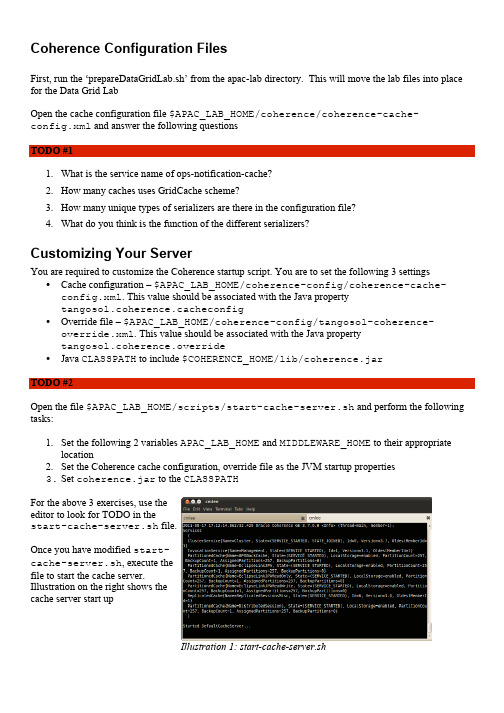
Coherence Configuration FilesFirst, run the ‘prepareDataGridLab.sh’ from the apac-lab directory. This will move the lab files into place for the Data Grid LabOpen the cache configuration file $APAC_LAB_HOME/coherence/coherence-cache-config.xml and answer the following questionsTODO #11.What is the service name of ops-notification-cache?2.How many caches uses GridCache scheme?3.How many unique types of serializers are there in the configuration file?4.What do you think is the function of the different serializers?Customizing Your ServerYou are required to customize the Coherence startup script. You are to set the following 3 settings •Cache configuration – $APAC_LAB_HOME/coherence-config/coherence-cache-config.xml. This value should be associated with the Java propertytangosol.coherence.cacheconfig•Override file – $APAC_LAB_HOME/coherence-config/tangosol-coherence-override.xml. This value should be associated with the Java propertytangosol.coherence.override•Java CLASSPATH to include $COHERENCE_HOME/lib/coherence.jarTODO #2Open the file $APAC_LAB_HOME/scripts/start-cache-server.sh and perform the following tasks:1.Set the following 2 variables APAC_LAB_HOME and MIDDLEWARE_HOME to their appropriatelocation2.Set the Coherence cache configuration, override file as the JVM startup properties3.Set coherence.jar to the CLASSPATHFor the above 3 exercises, use theeditor to look for TODO in thestart-cache-server.sh file.Once you have modified start-cache-server.sh, execute thefile to start the cache server.Illustration on the right shows thecache server start upIllustration 1: start-cache-server.shMonitoring Coherence CachesStart an instance of the cache server using theprevious start-cache-server.shscript. Start JRockit Mission Control usingthe command ‘jrmc’. Open Coherence'smonitoring screen by expanding Discovered→JDP. Right click on the node (batcomputerin the example to the left) and select StartConsoleExamine Runtime and MBeans.Answer the following questions.TODO #31.What are the Coherenceservices that are available?2.How do you know how manyCoherence nodes makes upthis cluster? Verify that bystarting another instance ofthe cache server.Starting the OPSNotificationWe will not run a simple Coherence desktop application thatfeature some of the functionality that we have look at in thepresentation.Run startOPSShipmentNotifier.sh in$APAC_LAB_HOME/scripts directory. A brown box iconwill install itself on your system tray. Right click on it. The menudoes the following•Add – adds a Shipment to the cache•Load – randomly generates a specified number of shipment and add them to the cache•Query – queries the cache•Process – perform a process on the cache•Enable Listener – enables notification.Illustration 2: JRockit Mission ControlIllustration 3: Examining the cache serverIllustration 4: OPS Notificationtray icon•Exit – shutdown the tray iconGenerating Test ShipmentsWe will insert some Shipment data into the cache. Select Load and generate 1000 (or more) shipments. TODO #41.Re-examine the Coherence MBeans in Mission Control. What has changed? (Hint: something elsehas been added)ing Mission Control find out how many nodes are there in the cluster? Explain what are theCoherence nodes.3.What are the common services in the 2 nodes? Why is there a discrepancy?4.How do you roughly know how many Shipment objects are in the cache? (Hint: the Shipment areadded to EclipseLinkJPA cache)5.Which method would you use for a bulk insert into the cache? Coherence documentations are under$COHERENCE_HOME/doc/api.Querying the Shipment CacheWe will now query the Shipment data that we have inserted intothe cache. Right click on the OPS Notification tray icon andselect Query. Select File → Load filter scripts... Navigate to$APAC_LAB_HOME/ops-shipment-notifier/filters directory and select the first scriptid.js.Click on Okay. A new dialog box will open with the list ofshipment that meets the filter criteria.Open the other two query parcelcount.js andparcelAndCity.js examine and run them as well.Open $COHERENCE_HOME/doc/api/index.html. Look at com.tangosol.util.filter package. Use the classes for the package to perform the following queriesTODO #51.Find all Shipment address to 'Fred Flintstone'2.Find all Shipment address to 'Fred Flintstone' who lives in 'Springfield' city3.Find all Shipment that has more than 3 parcels addressed to 'Fred Flintstone' who lives in'Springfield' city4.Find all Shipment that has been delivered to 'Fred Flintstone' who lives in 'Springfield' city withBASIC shipping service. (Hint: you must add the following line'importPackage(com.oracle.demo.ops.domain)')5.Make up some of your own filters if you have timeNote: when you are specifying integer use the Integer class, eg. new Integer(10) instead of just 10. List of getter methods for Shipment, Address and Parcel classes and ShippingServiceName and ParcelStatus enumerated type.•class Shipment◦public String getExternalReferenceId()◦public Address getToAddress()◦public Address getFromAddress()Illustration 5: Query editor◦ public ShippingServiceName getShippingServiceName() ◦ List<Parcel> getParcels() •class Address◦ public String getAddressee() ◦ public String getAddressLine1() ◦ public String getAddressLine2() ◦ public String getCity() ◦ public String getState()◦ public String getPostalCode() •class Parcel◦ public int getShipmentId() ◦ public String getContents() ◦ public int getHeight() ◦ public int getWidth() ◦ public int getLength() ◦ public int getWeight()◦ public ParcelStatus getParcelStatus() •enum ShippingServiceName ◦ BASIC◦ EXPEDITED ◦ NEXT_DAY_AIR •enum ParcelStatus◦ BILLING_INFO_RECEIVED ◦ PARCEL_RECEIVED ◦ IN_TRANSIT ◦ DELIVERED◦ DELIVERY_EXCEPTIONProcessProcess calculates the total weight of all Shipment with a certain number of Parcels going to a certain city. It uses aggregator to perform this task.TODO #61. Open ProcessFrame.java in$APAC_LAB_HOME/ops-shipment-notifier/src directory and find out what is the type returned by the aggregator.2. Optional: change the aggregator to include the heaviest and lightest shipment. Note: its easier to use NetBeansEventsEnable Shipment notification by right clicking on tray icon and select 'Enable Listener'. Now right click tray icon again and select Add. A dialog box shown in the illustration to the right will be displayed. Fill in the Shipment form and add a few Parcels. Select Okay to persist to cache.A dialog box will pop up notifying you of the new Shipment. We will use this feature with OPS application in anotherIllustration 6: Using aggregator Illustration 7: Add Shipment formexercise.TODO #7Open ProcessFrame.java in $APAC_LAB_HOME/ops-shipment-notifier/src directory and answer the following questions1.If you are writing another Coherence application joining this cluster, what is the name of the cacheyou would use so that the notifier will work with your application2.Under what situation will the notifier 'fire' viz. what sort of events will cause this notifier to becalled?AnswerTODO #11.OPSBackCache2.Four – Address, Parcel, Shipment, ShippingService3.Two – ConfigurablePofContext, WrapperSerializer4.To serialize Java objects. The function of the 2 types of serializers in the configuration arei.ConfigurablePofContext – for serializing Java objects into platform neutral formatii.WrapperSerializer – for serializing Entity relationshipsTODO #21.Check the directories with the instructor2.For override and cache configuration-Dtangosol.coherence.override=${DIR}/coherence-config/tangosol-coherence-override.xml-Dtangosol.coherence.cacheconfig=${DIR}/coherence-config/coherence-cache-config.xmlwhere ${DIR} is the root directory that contains coherence-config3.For CLASSPATH setting${COHERENCE_HOME}/lib/coherence.jarTODO #31.Right click in Discovered → JDP → node. Select Start Console. Select on MBeans. ExpandCoherence → Service → node number. See Illustration 82.Select Coherence → Cluster and expand Members. See Illustration 9Illustration 8: Coherence nodesIllustration 9: Coherence cluster with2 nodesTODO #41. Coherence → Cache and Coherence → StorageManager was created in the MBean Tree. Indicates that actual caches have been created. See Illustration 102. See TODO #3 2 above. One of the node is the cache server and the other is the ops-shipment-notifier3. OPSBackCache. You can also get the same information under Coherence → StorageManager → OPSBackCache → ops-notification-cache . The second node only creates ops-notification-cache . See Illustration 114. Expand Coherence → Cache → EclipseLinkJPA → node → back → Shipment. Look at Units.5. NamedCache.putAll()TODO #5Query 1 filter = new LikeFilter("getToAddress.getAddressee" , "Fred Flintstone")Query 2 nameFilter = new LikeFilter("getToAddress.getAddressee" , "Fred Flintstone") cityFilter = new LikeFilter("getToAddress.getCity" , "Springfield") filter = new AndFilter(cityFilter, nameFilter)Query 3 nameFilter = new LikeFilter("getToAddress.getAddressee" , "Fred Flintstone") cityFilter = new LikeFilter("getToAddress.getCity" , "Springfield") parcelCount = new GreaterEqualsFilter("getParcels.size" , new Integer(3)) filter = new AndFilter(new AndFilter(cityFilter, nameFilter) , parcelCount)Illustration 10: Additional nodes: Cache, StorageManager Illustration 11:OPSBackCache under node 1 and 2Query 4importPackage(com.oracle.demo.ops.domain)nameFilter = new LikeFilter("getToAddress.getAddressee", "Fred Flintstone")cityFilter = new LikeFilter("getToAddress.getCity", "Springfield")shipmentServiceFilter = new EqualsFilter("getShippingServiceName", ShippingServiceName.BASIC)filter = new AndFilter(new AndFilter(cityFilter, nameFilter) , shipmentServiceFilter)TODO #61.Map<String, Object>2.Edit CalculateWeightAggregrator@Overridepublic Object aggregate(Set setEntries) {Map<String, Object> result = new HashMap<String, Object>();int total = 0;int heaviest = 0;int lightest = 1000;result.put(Constants.TOTAL_ENTRY, setEntries.size());for (Object o: setEntries) {InvocableMapHelper.SimpleEntry entry =(InvocableMapHelper.SimpleEntry)o;Shipment s = (Shipment)entry.getValue();for (Parcel p: s.getParcels()) {int weight = p.getWeight();total += weight;if (weight > heaviest)heaviest = weight;else if (weight < lightest)lightest = weight;}}result.put(Constants.TOTAL_WEIGHT, total);result.put("heaviestParcel", heaviest);result.put("lightestParcel", lightest);return (result);}TODO #71.ops-notification-cache. From OpsShipmentNotifier.java.2.When Shipment are updated or inserted. ShipmentListenerImpl.java implements aFilter which defines this predicate。
lab2-2三级跳
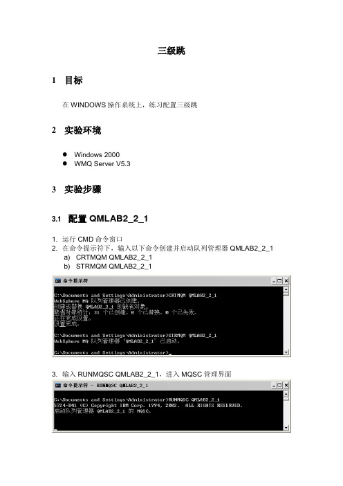
三级跳1目标在WINDOWS操作系统上,练习配置三级跳2实验环境●Windows 2000●WMQ Server V5.33实验步骤3.1 配置QMLAB2_2_11. 运行CMD命令窗口2. 在命令提示符下,输入以下命令创建并启动队列管理器QMLAB2_2_1a) CRTMQM QMLAB2_2_1b) STRMQM QMLAB2_2_13. 输入RUNMQSC QMLAB2_2_1,进入MQSC管理界面4. 在MQSC中,输入如下命令a) DEFINE QREMOTE(RQ.QMLAB2_2_3) RNAME(LQ.QMLAB2_2_3)RQMNAME(QMLAB2_2_3) XMITQ(QMLAB2_2_2)b) DEFINE QLOCAL(QMLAB2_2_2) USAGE(XMITQ)c) DEFINE CHANNEL(TO.QMLAB2_2_2) CHLTYPE(SDR)TRPTYPE(TCP) CONNAME(‘127.0.0.1(1416)’)XMITQ(QMLAB2_2_2)d) END3.2 配置QMLAB2_2_21. 运行CMD命令窗口2. 在命令提示符下,输入以下命令创建并启动队列管理器QMLAB2_2_2a) CRTMQM QMLAB2_2_2b) STRMQM QMLAB2_2_23. 输入RUNMQSC QMLAB2_2_2,进入MQSC管理界面4. 在MQSC中,输入如下命令a) DEFINE QLOCAL(QMLAB2_2_3) USAGE (XMITQ)b) DEFINE CHANNEL(TO.QMLAB2_2_2) CHLTYPE(RCVR)TRPTYPE(TCP)c) DEFINE CHANNEL(TO.QMLAB2_2_3) CHLTYPE(SDR)TRPTYPE(TCP) CONNAME(‘127.0.0.1(1417)’)XMITQ(QMLAB2_2_3)d) END3.3 配置QMLAB2_2_31. 运行CMD命令窗口2. 在命令提示符下,输入以下命令创建并启动队列管理器QMLAB2_2_3a) CRTMQM QMLAB2_2_3b) STRMQM QMLAB2_2_33. 输入RUNMQSC QMLAB2_2_3,进入MQSC管理界面4. 在MQSC中,输入如下命令e) DEFINE QLOCAL(LQ.QMLAB2_2_3)f) DEFINE CHANNEL(TO.QMLAB2_2_3) CHLTYPE(RCVR)TRPTYPE(TCP)g) END3.4 启动1. 在命令提示符下,输入a) runmqlsr -m QMLAB2_2_2 -t tcp -p 1416,启动侦听器b) runmqlsr -m QMLAB2_2_3 -t tcp -p 1417,启动侦听器c) runmqchl -m QMLAB2_2_1 -c TO.QMLAB2_2_2,启动通道d) runmqchl -m QMLAB2_2_2 -c TO.QMLAB2_2_3,启动通道2. 输入amqsput RQ.QMLAB2_2_3 QMLAB2_2_1,放入消息3. 输入amqsget LQ.QMLAB2_2_3 QMLAB2_2_3,取出消息。
CS144学习(2)TCP协议实现
CS144学习(2)TCP协议实现Lab1-4 分别是完成⼀个流重组器,TCP接收端,TCP发送端,TCP连接四个部分,将四个部分组合在⼀起就是⼀个完整的TCP端了。
之后经过包装就可以进⾏TCP的接收和发送了。
代码全部在上了。
Lab1 流重组器这⼀个实验是要实现⼀个流重组器,传⼊数据的⽚段以及起始位置,之后对其进⾏重组,并尽快将以及重组完成的数据输出。
这⾥我使⽤的是红⿊树来实现,也就是C++的std::set来实现。
将未重组完成的碎⽚保存在红⿊树中,当新碎⽚到达时就尽可能地将该碎⽚与已有的碎⽚进⾏合并,保证红⿊树中没有重叠的碎⽚。
这⼀个实验的问题就是要考虑的情况有很多,当⽤lower_bound()找到插⼊位置后,要对前⾯和后⾯的碎⽚判断能否合并,合并的情况也有很多种,包括部分重叠、正好接上、完全覆盖等情况;⽽且⼀个新的碎⽚可能会⼀次覆盖掉很多碎⽚。
这⼀部分代码我写的⽐较混乱,因为写完之后测试发现有情况没考虑到,然后就只能打补丁,于是就越来越混乱了。
⽽尽快输出这个条件还是很容易的,如果当前到达碎⽚能够直接输出的话,就再判断⼀下树中第⼀个碎⽚能否输出,因为前⾯保证了不会有重叠碎⽚,所以可以只对第⼀个碎⽚进⾏判断。
Lab2 TCP接收端这个实验是基于上⼀个的流重组器来实现⼀个TCP接收端,这⼀个还是⽐较简单的。
就是前⾯流重组器的⼀些BUG可能会在这个实验⾥⾯被检测到,要回去改代码。
⾸先是实现⼀个WrappingInt32,因为TCP的序号是32位的,并且是可能发⽣溢出的,⽽在流重组器⾥⾯使⽤的序列号是64位,因此需要实现函数来进⾏转换,将64位的相对序列号根据ISN转换成32位的绝对序列号。
#include "wrapping_integers.hh"using namespace std;WrappingInt32 wrap(uint64_t n, WrappingInt32 isn) {uint64_t res = isn.raw_value() + n;return WrappingInt32{static_cast<uint32_t>(res)};}uint64_t abs(uint64_t a, uint64_t b) {if (a > b) {return a - b;} else {return b - a;}}uint64_t unwrap(WrappingInt32 n, WrappingInt32 isn, uint64_t checkpoint) {uint64_t pre = checkpoint & 0xffffffff00000000;uint64_t num;if (n.raw_value() >= isn.raw_value()) {num = n.raw_value() - isn.raw_value();} else {num = 0x0000000100000000;num += n.raw_value();num -= isn.raw_value();}uint64_t a = pre + num;uint64_t b = a + 0x0000000100000000;uint64_t c = a - 0x0000000100000000;// b a cif (abs(a, checkpoint) < abs(b, checkpoint)) {if (abs(a, checkpoint) < abs(c, checkpoint)) {return a;} else {return c;}} else {return b;}}最后就是对流重组器进⾏⼀下包装,计算出ackno和window_size提供给后⾯使⽤,处理⼀下SYN和FIN标记就⾏了。
Lab 2
Lab 2VelocityOverviewIn this lab, we will explore the relationship between the position function and the velocity function of a moving object. In the lectures, we have seen that the velocity function v(t) is the derivative of the position function s(t) (and therefore s(t) is an antiderivative ofv(t)). We will be examining these statements in this lab by using a motion detector to measure the velocity and position of a person walking.Vocabulary used in this lab•Distance: This is the distance an object is from the motion detector. The words distance and position will be used interchangeably in this lab.•Displacement: This is “change of position,” that is, the difference between the initial and terminal coordinates the object. Displacement can be either positive or negative. (Think about what the difference between positive and negativedisplacement is.)•Velocity and speed: The important thing to note here is that velocity can be either positive or negative, depending on whether motion is in the positive ornegative direction. But speed = |v(t)| is never negative: it is the absolute value of the velocity. For example, a car’s speedometer is measuring speed and alwaysreads positive, regardless of the direction you’re traveling.•Total distance traveled: Perhaps this is best illustrated by an example. If you walk 2 meters forward and then 2 meters backward then your displacement willzero (the initial and terminal positions are the same so therefore the difference of coordinates is zero). But, you actually traveled 4 meters. In this case, the totaldistance traveled would be 4 meters. The “total distance traveled” is nevernegative.Mathematics for this labThe mathematics that we will need is the relationship between displacement and velocity: •Displacement is equal to the definite integral of velocity v(t) over a time interval.•Total distance traveled is equal to the definite integral of speed |v(t)|over a time interval.These ideas are discussed in the textbook on pages 374-375.Materials•Computer with Vernier computer interface.•Vernier motion detector. This will plug into the LoggerPro computer interface.•Separate “Lab Report 2” sheet. This is what you will turn in. It is due one week after your scheduled lab day, by 4:30 pm, in the Mathematics Office (Cupples I,room 100).Comments on the Motion DetectorThe motion detector works by emitting short bursts of ultrasonic sound waves. You will hear a clicking sound when the detector is operating. The detector “listens” for the ech o of these ultrasonic waves returning to it. The motion detector measures the time it takes for the sound waves to make the trip from the detector to the object and back to the detector. Knowing the speed of sound, the detector is then able to calculate the distance to the object.The specifications on the detector state that it has a minimum range of 0.4 m. and a maximum range of 6.0 m. The detector seems to work best if there is a smooth flat surface for the sound waves to bounce off of.Practically speaking, this means that as you collect data•Your motion needs to be parallel to the sensor and not perpendicular to it (i.e., you will need to walk either away from or towards the sensor, or both).•You will probably want to be holding a book or piece of cardboard in the sensor’s “line of sight” while you walk.•If neighboring lab teams are moving while you are collecting data, your motion detector might pick up their motion as well. You will have to cooperate with your neighboring teams so that your motion detector is only picking up data from your walking.•It is very important that the motion detector does not move. (What would the motion detector measure if it was moving?)ProcedureThe first thing to do is get the computer and motion detector ready.Connect the motion detector to the Dig/Sonic 2 port of the Lab Pro. Make sure the Lab Pro is connected to the USB port of the computer. (It is likely that these have already been done for you.)•Set the detector upright on the edge of the desk, facing out in a direction in which you have a clear path at least 2 m. long.•Open the LoggerPro program. You will want to select “Lab Pro USB” for the port in the Setup Interface. It is possible (hopefully not likely) that LoggerProwill not recognize the hardware. If this happens, unplugging the Lab Pro andplugging it back in should take care of the problem.•Open the experiment file for this lab. (Click on the “Open” button and open the file labeled “lab2_velocity.” (It is possible that LoggerPro will complain aboutthis file – just ignore any complaint and click “OK.”)•At this point, you should be able to collect distance and velocity data. Try playing around with the motion detector by pressing the “collect button” on thetoolbar. (For example: turn the sensor to face the nearest wall and collect data—what happens? Turn the sensor around and collect data by moving your handback-and-forth in front of it.) When you start collecting data, notice that velocity and distance data is graphed and the actual data appears in a table to the right ofthe graphs. Notice also that each time you start collecting new data, the data from the previous run is cleared. (Another way to clear recently collected data is toselect Data, Delete Run from the menu.)You are now ready to start collecting data that you will analyze.•Decide who will monitor the computer (and hit the collect button) and who will be the “mover”—the mover will create distance and velocity data bywalking back and forth in front of the motion detector.•Your goal is to generate a data set that exhibits both positive and negative velocity during the five seconds of movement.•There is a limited amount of free space in the lab for straight-line movement, so you will have to coordinate your data collection with your neighbors.Make sure you have a clear path before you start collecting your data.•The mover should take an initial position standing in front of the motion detector, holding a book or a piece of cardboard in the detector’s “line ofsight.” This will help to make a smoother velocity graph as you collect thedata.Before beginning, note the mover’s initial position. When the datacollection stops, the mover should remain in position while his/her partnernotes the terminal position. (An acceptable method to note these positionsis to put a marker, like a pen, on the floor where the mover’s feet start.)Measure and write down these positions (number of meters in front of thesensor); you’ll need this information later. (There will be a tape measurein the lab for you to measure the distances. You’re not looking for greataccuracy—just something in the right ballpark. Remember that 1 meter isapproximately 3.28 feet.).•Click on the “Collect” button and gather the data. When the mover hears the motion detector making the clicking sound, s/he should start moving along astraight line in front of the motion detector. Remember your goal to createdata with positive and negative velocity.After collecting your distance and velocity data, you should make sure your data looks “reasonable”: for example,•Is the graph of the velocity reasonably smooth?•Does the distance data in the table look like what you were expecting? Do the distances more-or-less match up with what you noted for the initial and finalpositions?•Is the velocity positive and negative when you were expecting it to be positive and negative?•If your data looks questionable, collect another set of data. (The good news is that it doesn’t take much time to collect another data set if necessary.) •If your data looks good, save it so that you can finish your report after the lab period if necessary. (If you didn’t bring a diskette, you could e-mail the datato yourself.)At this point, you are ready to analyze your data.•You should have two graphs –position (labeled “Distance vs. Time”) and velocity (labeled “Velocity vs. Time). You should print both of these graphs and also the table: activate each graph or table window before you print (so that youget a nice printout of each one separately).•Click on the “Examine” button (Analyze – Examine in the menu). This should allow you to more easily read both the graph and the data (watch what happenswhen you move the mouse to the graphs and the data table). Using this, answer#1-3 on Lab Report 2.DisplacementWe want to calculate the displacement of the mover after 5 seconds. We can do this in three different ways:a) by having LoggerPro estimate the integral of the velocityfunction v(t) for 0 <= t <= 5b) by using our data and the Fundamental Theorem of Calculus (Part II) to evaluate the same integralc) by using the measurements we made “by hand” during the data collection process.In detail:a) Using LoggerPro to estimate the integral of the velocity:•Click on the left-hand side of the velocity graph (Time=0) and drag the black line across to the right-hand side of the graph. While you are doing this, the values in the table window should be highlighted. Make sure you actually click on thegraph on not outside the graph (otherwise you will see the pop-up box asking you about the y-axis and y-scale).•Click the Integral button or choose Analyze – Integrate from the menu. A floating box with LoggerPro’s estimate of the value of the integral appears in the Veloci ty graph window. Note the units in this box: m/s * s, which is just meters (theseconds cancel out); don’t misread the units as “m/sec2” !! Print a copy of thegraph with the box. Record this value in #4a on the Lab Report.b) According the Fundamental Theorem of Calculus (Part II), we can compute the integral of v(t) over the time interval [0,5] using an antiderivative. In this situation, the numeric result can be worked out using subtracting two numbers taken from your data tables. In the Lab Report #4b state what numbers you are using and give the resulting value for the integral.c) Finally, calculate the displacement using the distances from the sensor that you measured during the data collection process. Record the result of the calculation in Lab Report #4c.In Lab Report #4d, you are asked to offer some reasons why the results in a), b) and c) are (probably) not equal.Total Distance TraveledTo find the total distance traveled, we need to integrate the speed |v(t)| during our 5 second time interval. To have LoggerPro do this,we need the speed data—so we create it in a new column:•Activate the velocity graph window by clicking on the velocity graph. Select View – Graph Options from the menu.•Modify the Graph Title by typing “Speed/” before Velocity. It should now read Speed/Velocity vs. Time. Click Apply, then click OK.•Select Data - New Column, Formula from the Data menu. The New Column window will appear.•Under the Options tab, in the Labels section, type “Speed” for Long Name, “sp”for Short Name and “m/s” for Units.•Click the Definition tab. In the Equation box, enter the formula(abs(“Velocity”)). You can (and should) do this by selecting “abs()” from the Functions list followed by selecting “Velocity” from the Variables list.•Click Try New Column. If it new data looks as it should (how should it look?), then click “OK”.•Notice that the new graph (Speed) coincides with the original velocity graph when the velocity is positive. How do these graphs compare when velocity is negative? •Click on the left-hand side of the speed/velocity graph (Time = 0) and drag the black line across to the right-hand side of the graph. All of the values in the table window should be highlighted.•Click the Integrate button. An Integral Selection window appears. Remove the check next to Velocity by clicking in its box. Make sure that Speed is checked.Click OK.• A floating box with LoggerPro’s estimate of the value of the integral appears in the Speed/Velocity graph window. Print a copy of the graph with the box. Report the total distance traveled on Lab Report, #5.Answer #6 and #7 on the Lab Report sheet.。
lab_guide_2_TAMeb_installation
TAM/TIM Workshop Lab Guide-22 TAM for e-business的安装 (3)2.1 安装IBM Java Runtime (3)2.2 安装Policy Server (3)2.3 配置Policy Server (11)2.4 安装Webseal (14)2.5 配置Webseal (21)2.6 访问webseal (22)2.7 安装TAM authorization Server (23)2.8 配置TAM authorization Server (26)2.9 安装WPM (27)2.10 访问WPM (33)2TAM for e-business的安装==Notes==TAM for e-business分为两个介质包,分别为BASE和WEB。
其中Policy Server的介质在BASE包中,WebSeal的介质在WEB_SECURITY包中。
2.1安装IBM Java Runtime1)安装介质在base介质包的linux_i386路径下2)设置PATH变量2.2安装Policy Server运行./install_ammg,安装过程中会安装如下组件:z IBM Global Security Kit (GSKit)z IBM Tivoli Directory Server base client (as needed)z IBM Tivoli Directory Server 32-bit client (as needed)z Tivoli Security Utilitiesz Tivoli Access Manager Access Manager Licensez Tivoli Access Manager Access Manager Runtimez Tivoli Access Manager Access Manager Policy Server选择LDAP 作为Registry:填写LDAP所在主机的主机名(不要使用IP地址):填入TAM管理员密码,passw0rd;端口保留默认值:填入LDAP的密码:passw0rd;接受默认domain名字:下面保留默认值:==Notes==安装过程中,安装wizard还会配置Policy server和相应的组件。
湖南大学计组实验lab2 datalab
4 bitCount 函数 /* * bitCount - returns count of number of 1's in word
* Examples: bitCount(5) = 2, bitCount(7) = 3 * Legal ops: ! ~ & ^ | + << >> * Max ops: 40 * Rating: 4 */ int bitCount(int x) { int tmp=(((0x01<<8|0x01)<<8|0x01)<<8|0x01)<<8|0x01; int val=tmp&x; //检测 x 的 0,8,16,24 位是否为 1 val+=tmp&(x>>1); //检测 x 的 1,9,17,25 位是否为 1 val+=tmp&(x>>2); //... val+=tmp&(x>>3); val+=tmp&(x>>4); val+=tmp&(x>>5); val+=tmp&(x>>6); val+=tmp&(x>>7); //检测 x 的 7,15,23,31 位是否为 1 val+=(val>>16); //将 val 的高 16 位加到低 16 位上 val+=(val>>8); //再将 val 的高 8 位加到低 8 位上 return val&0xff; //保留 val 的最低 byte 信息 为最终结果} 代码思路:检测数据里有多少个 1,如果每一位作检测的话,肯定会超出操作符 限制,所以考虑一次检查多个,那么应该怎样做? 这里考虑一个数 0000 0001 0000 0001 0000 0001 0000 0001,将它与一个数作& 操作,即可判定在这个数的 0,8,16,24 位有多少个 1,接下来,将待检测的数作移 位操作,还可以继续用这种方法检测,将检测后的所有结果累加,每 8 位作为一个单 元,将总数相加,就可以得到我们需要的总的 1 的个数。
- 1、下载文档前请自行甄别文档内容的完整性,平台不提供额外的编辑、内容补充、找答案等附加服务。
- 2、"仅部分预览"的文档,不可在线预览部分如存在完整性等问题,可反馈申请退款(可完整预览的文档不适用该条件!)。
- 3、如文档侵犯您的权益,请联系客服反馈,我们会尽快为您处理(人工客服工作时间:9:00-18:30)。
1
实验二 一元回归模型
【实验目的】
掌握一元线性、非线性回归模型的建模方法
【实验内容】
建立我国税收预测模型
【实验步骤】
【例1】建立我国税收预测模型。表1列出了我国1985-1998年间税收收入Y和国内生产
总值(GDP)x的时间序列数据,请利用统计软件Eviews建立一元线性回归模型。
表1 我国税收与GDP统计资料
年份 税收 GDP 年份 税收 GDP
1985 2041 8964 1992 3297 26638
1986 2091 10202 1993 4255 34634
1987 2140 11963 1994 5127 46759
1988 2391 14928 1995 6038 58478
1989 2727 16909 1996 6910 67885
1990 2822 18548 1997 8234 74463
1991 2990 21618 1998 9263 79396
一、建立工作文件
⒈菜单方式
在录入和分析数据之前,应先创建一个工作文件(Workfile)。启动Eviews软件之后,
在主菜单上依次点击File\New\Workfile(菜单选择方式如图1所示),将弹出一个对话框(如
图2所示)。用户可以选择数据的时间频率(Frequency)、起始期和终止期。
图1 Eviews菜单方式创建工作文件示意图
2
图2 工作文件定义对话框
本例中选择时间频率为Annual(年度数据),在起始栏和终止栏分别输入相应的日期85
和98。然后点击OK,在Eviews软件的主显示窗口将显示相应的工作文件窗口(如图3所
示)。
图3 Eviews工作文件窗口
一个新建的工作文件窗口内只有2个对象(Object),分别为c(系数向量)和resid(残
差)。它们当前的取值分别是0和NA(空值)。可以通过鼠标左键双击对象名打开该对象查
看其数据,也可以用相同的方法查看工作文件窗口中其它对象的数值。
⒉命令方式
还可以用输入命令的方式建立工作文件。在Eviews软件的命令窗口中直接键入
CREATE命令,其格式为:
CREATE 时间频率类型 起始期 终止期
本例应为:CREATE A 85 98
二、输入数据
在Eviews软件的命令窗口中键入数据输入/编辑命令:
DATA Y X
此时将显示一个数组窗口(如图4所示),即可以输入每个变量的数值
3
图4 Eviews数组窗口
三、图形分析
借助图形分析可以直观地观察经济变量的变动规律和相关关系,以便合理地确定模型的
数学形式。
⒈趋势图分析
命令格式:PLOT 变量1 变量2 ……变量K
作用:⑴分析经济变量的发展变化趋势
⑵观察是否存在异常值
本例为:PLOT Y X
⒉相关图分析
命令格式:SCAT 变量1 变量2
作用:⑴观察变量之间的相关程度
⑵观察变量之间的相关类型,即为线性相关还是曲线相关,曲线相关时大致是哪
种类型的曲线
说明:⑴SCAT命令中,第一个变量为横轴变量,一般取为解释变量;第二个变量为纵
轴变量,一般取为被解释变量
⑵SCAT命令每次只能显示两个变量之间的相关图,若模型中含有多个解释变
量,可以逐个进行分析
⑶通过改变图形的类型,可以将趋势图转变为相关图
本例为:SCAT Y X
图5 税收与GDP趋势图
图5、图6分别是我国税收与GDP时间序列趋势图和相关图分析结果。两变量趋势图
4
分析结果显示,我国税收收入与GDP二者存在差距逐渐增大的增长趋势。相关图分析显示,
我国税收收入增长与GDP密切相关,二者为非线性的曲线相关关系。
图6 税收与GDP相关图
三、估计线性回归模型
在数组窗口中点击Proc\Make Equation,如果不需要重新确定方程中的变量或调整样本
区间,可以直接点击OK进行估计。也可以在Eviews主窗口中点击Quick\Estimate Equation,
在弹出的方程设定框(图7)内输入模型:
Y C X
图7 方程设定对话框
还可以通过在Eviews命令窗口中键入LS命令来估计模型,其命令格式为:
LS 被解释变量 C 解释变量
系统将弹出一个窗口来显示有关估计结果(如图8所示)。因此,我国税收模型的估计
式为:
xy0946.054.987ˆ
这个估计结果表明,GDP每增长1亿元,我国税收收入将增加0.09646亿元。
5
图8 我国税收预测模型的输出结果
五、估计非线性回归模型
由相关图分析可知,变量之间是非线性的曲线相关关系。因此,可初步将模型设定为指
数函数模型、对数模型和二次函数模型并分别进行估计。
在Eviews命令窗口中分别键入以下命令命令来估计模型:
双对数函数模型:LS log(Y) C log(X)
对数函数模型:LS Y C log(X)
指数函数模型:LS log(Y) C X
二次函数模型:LS Y C X X^2
还可以采取菜单方式,在上述已经估计过的线性方程窗口中点击Estimate项,然后在弹
出的方程定义窗口中依次输入上述模型(方法通线性方程的估计),其估计结果显示如图9、
图10、图11图、12所示。
双对数模型:xyln6823.02704.1ˆln
(3.8305) (21.0487)
9736.02R 9714.02R
05.443F
对数模型:xyln92.298532.26163ˆ
(-8.3066) (9.6999)
8869.02R 8775.02R
0875.94F
指数模型:xy51007.25086.7ˆln
(231.7463) (27.2685)
9841.02R 9828.02R
57.743F
二次函数模型:271058.50468.07.1645ˆxxy
(7.4918) (3.3422) (3.4806)
9918.02R 9903.02R
78.661F
6
图9 双对数模型回归结果
图10 对数模型回归结果
图11 指数模型回归结果
7
图12 二次函数模型回归结果
六、模型比较
四个模型的经济意义都比较合理,解释变量也都通过了T检验。但是从模型的拟合优
度来看,二次函数模型的2R值最大,其次为指数函数模型。因此,对这两个模型再做进一
步比较。
在回归方程(以二次函数模型为例)窗口中点击View\Actual,Fitted,Residual\
Actual,Fitted,Residual Table(如图13),可以得到相应的残差分布表。
图13 回归方程残差分析菜单
上述两个回归模型的残差分别表分别如下(图14、图15)。比较两表可以发现,虽然二
次函数模型总拟合误差较小,但其近期误差却比指数函数模型大。所以,如果所建立的模型
是用于经济预测,则指数函数模型更加适合。
8
图14 二次函数回归模型残差分别表
图15 指数函数模型残差分布表