A Robust Decision Tree Algorithm for Imbalanced Data Sets (2)
外文文献文献列表

- disruption ,: Global convergence vs nationalSustainable - ,practices and dynamic capabilities in the food industry: A critical analysis of the literature5 Mesoscopic - simulation6 Firm size and sustainable performance in food -s: Insights from Greek SMEs7 An analytical method for cost analysis in multi-stage -s: A stochastic / model approach8 A Roadmap to Green - System through Enterprise Resource Planning (ERP) Implementation9 Unidirectional transshipment policies in a dual-channel -10 Decentralized and centralized model predictive control to reduce the bullwhip effect in - ,11 An agent-based distributed computational experiment framework for virtual - / development12 Biomass-to-bioenergy and biofuel - optimization: Overview, key issues and challenges13 The benefits of - visibility: A value assessment model14 An Institutional Theory perspective on sustainable practices across the dairy -15 Two-stage stochastic programming - model for biodiesel production via wastewater treatment16 Technology scale and -s in a secure, affordable and low carbon energy transition17 Multi-period design and planning of closed-loop -s with uncertain supply and demand18 Quality control in food - ,: An analytical model and case study of the adulterated milk incident in China19 - information capabilities and performance outcomes: An empirical study of Korean steel suppliers20 A game-based approach towards facilitating decision making for perishable products: An example of blood -21 - design under quality disruptions and tainted materials delivery22 A two-level replenishment frequency model for TOC - replenishment systems under capacity constraint23 - dynamics and the ―cross-border effect‖: The U.S.–Mexican border’s case24 Designing a new - for competition against an existing -25 Universal supplier selection via multi-dimensional auction mechanisms for two-way competition in oligopoly market of -26 Using TODIM to evaluate green - practices under uncertainty27 - downsizing under bankruptcy: A robust optimization approach28 Coordination mechanism for a deteriorating item in a two-level - system29 An accelerated Benders decomposition algorithm for sustainable - / design under uncertainty: A case study of medical needle and syringe -30 Bullwhip Effect Study in a Constrained -31 Two-echelon multiple-vehicle location–routing problem with time windows for optimization of sustainable - / of perishable food32 Research on pricing and coordination strategy of green - under hybrid production mode33 Agent-system co-development in - research: Propositions and demonstrative findings34 Tactical ,for coordinated -s35 Photovoltaic - coordination with strategic consumers in China36 Coordinating supplier׳s reorder point: A coordination mechanism for -s with long supplier lead time37 Assessment and optimization of forest biomass -s from economic, social and environmental perspectives – A review of literature38 The effects of a trust mechanism on a dynamic - /39 Economic and environmental assessment of reusable plastic containers: A food catering - case study40 Competitive pricing and ordering decisions in a multiple-channel -41 Pricing in a - for auction bidding under information asymmetry42 Dynamic analysis of feasibility in ethanol - for biofuel production in Mexico43 The impact of partial information sharing in a two-echelon -44 Choice of - governance: Self-managing or outsourcing?45 Joint production and delivery lot sizing for a make-to-order producer–buyer - with transportation cost46 Hybrid algorithm for a vendor managed inventory system in a two-echelon -47 Traceability in a food -: Safety and quality perspectives48 Transferring and sharing exchange-rate risk in a risk-averse - of a multinational firm49 Analyzing the impacts of carbon regulatory mechanisms on supplier and mode selection decisions: An application to a biofuel -50 Product quality and return policy in a - under risk aversion of a supplier51 Mining logistics data to assure the quality in a sustainable food -: A case in the red wine industry52 Biomass - optimisation for Organosolv-based biorefineries53 Exact solutions to the - equations for arbitrary, time-dependent demands54 Designing a sustainable closed-loop - / based on triple bottom line approach: A comparison of metaheuristics hybridization techniques55 A study of the LCA based biofuel - multi-objective optimization model with multi-conversion paths in China56 A hybrid two-stock inventory control model for a reverse -57 Dynamics of judicial service -s58 Optimizing an integrated vendor-managed inventory system for a single-vendor two-buyer - with determining weighting factor for vendor׳s ordering59 Measuring - Resilience Using a Deterministic Modeling Approach60 A LCA Based Biofuel - Analysis Framework61 A neo-institutional perspective of -s and energy security: Bioenergy in the UK62 Modified penalty function method for optimal social welfare of electric power - with transmission constraints63 Optimization of blood - with shortened shelf lives and ABO compatibility64 Diversified firms on dynamical - cope with financial crisis better65 Securitization of energy -s in China66 Optimal design of the auto parts - for JIT operations: Sequential bifurcation factor screening and multi-response surface methodology67 Achieving sustainable -s through energy justice68 - agility: Securing performance for Chinese manufacturers69 Energy price risk and the sustainability of demand side -s70 Strategic and tactical mathematical programming models within the crude oil - context - A review71 An analysis of the structural complexity of - /s72 Business process re-design methodology to support - integration73 Could - technology improve food operators’ innovativeness? A developing country’s perspective74 RFID-enabled process reengineering of closed-loop -s in the healthcare industry of Singapore75 Order-Up-To policies in Information Exchange -s76 Robust design and operations of hydrocarbon biofuel - integrating with existing petroleum refineries considering unit cost objective77 Trade-offs in - transparency: the case of Nudie Jeans78 Healthcare - operations: Why are doctors reluctant to consolidate?79 Impact on the optimal design of bioethanol -s by a new European Commission proposal80 Managerial research on the pharmaceutical - – A critical review and some insights for future directions81 - performance evaluation with data envelopment analysis and balanced scorecard approach82 Integrated - design for commodity chemicals production via woody biomass fast pyrolysis and upgrading83 Governance of sustainable -s in the fast fashion industry84 Temperature ,for the quality assurance of a perishable food -85 Modeling of biomass-to-energy - operations: Applications, challenges and research directions86 Assessing Risk Factors in Collaborative - with the Analytic Hierarchy Process (AHP)87 Random / models and sensitivity algorithms for the analysis of ordering time and inventory state in multi-stage -s88 Information sharing and collaborative behaviors in enabling - performance: A social exchange perspective89 The coordinating contracts for a fuzzy - with effort and price dependent demand90 Criticality analysis and the -: Leveraging representational assurance91 Economic model predictive control for inventory ,in -s92 - ,ontology from an ontology engineering perspective93 Surplus division and investment incentives in -s: A biform-game analysis94 Biofuels for road transport: Analysing evolving -s in Sweden from an energy security perspective95 - ,executives in corporate upper echelons Original Research Article96 Sustainable - ,in the fast fashion industry: An analysis of corporate reports97 An improved method for managing catastrophic - disruptions98 The equilibrium of closed-loop - super/ with time-dependent parameters99 A bi-objective stochastic programming model for a centralized green - with deteriorating products100 Simultaneous control of vehicle routing and inventory for dynamic inbound -101 Environmental impacts of roundwood - options in Michigan: life-cycle assessment of harvest and transport stages102 A recovery mechanism for a two echelon - system under supply disruption103 Challenges and Competitiveness Indicators for the Sustainable Development of the - in Food Industry104 Is doing more doing better? The relationship between responsible - ,and corporate reputation105 Connecting product design, process and - decisions to strengthen global - capabilities106 A computational study for common / design in multi-commodity -s107 Optimal production and procurement decisions in a - with an option contract and partial backordering under uncertainties108 Methods to optimise the design and ,of biomass-for-bioenergy -s: A review109 Reverse - coordination by revenue sharing contract: A case for the personal computers industry110 SCOlog: A logic-based approach to analysing - operation dynamics111 Removing the blinders: A literature review on the potential of nanoscale technologies for the ,of -s112 Transition inertia due to competition in -s with remanufacturing and recycling: A systems dynamics mode113 Optimal design of advanced drop-in hydrocarbon biofuel - integrating with existing petroleum refineries under uncertainty114 Revenue-sharing contracts across an extended -115 An integrated revenue sharing and quantity discounts contract for coordinating a - dealing with short life-cycle products116 Total JIT (T-JIT) and its impact on - competency and organizational performance117 Logistical - design for bioeconomy applications118 A note on ―Quality investment and inspection policy in a supplier-manufacturer -‖119 Developing a Resilient -120 Cyber - risk ,: Revolutionizing the strategic control of critical IT systems121 Defining value chain architectures: Linking strategic value creation to operational - design122 Aligning the sustainable - to green marketing needs: A case study123 Decision support and intelligent systems in the textile and apparel -: An academic review of research articles124 - ,capability of small and medium sized family businesses in India: A multiple case study approach125 - collaboration: Impact of success in long-term partnerships126 Collaboration capacity for sustainable - ,: small and medium-sized enterprises in Mexico127 Advanced traceability system in aquaculture -128 - information systems strategy: Impacts on - performance and firm performance129 Performance of - collaboration – A simulation study130 Coordinating a three-level - with delay in payments and a discounted interest rate131 An integrated framework for agent basedinventory–production–transportation modeling and distributed simulation of -s132 Optimal - design and ,over a multi-period horizon under demand uncertainty. Part I: MINLP and MILP models133 The impact of knowledge transfer and complexity on - flexibility: A knowledge-based view134 An innovative - performance measurement system incorporating Research and Development (R&D) and marketing policy135 Robust decision making for hybrid process - systems via model predictive control136 Combined pricing and - operations under price-dependent stochastic demand137 Balancing - competitiveness and robustness through ―virtual dual sourcing‖: Lessons from the Great East Japan Earthquake138 Solving a tri-objective - problem with modified NSGA-II algorithm 139 Sustaining long-term - partnerships using price-only contracts 140 On the impact of advertising initiatives in -s141 A typology of the situations of cooperation in -s142 A structured analysis of operations and - ,research in healthcare (1982–2011143 - practice and information quality: A - strategy study144 Manufacturer's pricing strategy in a two-level - with competing retailers and advertising cost dependent demand145 Closed-loop - / design under a fuzzy environment146 Timing and eco(nomic) efficiency of climate-friendly investments in -s147 Post-seismic - risk ,: A system dynamics disruption analysis approach for inventory and logistics planning148 The relationship between legitimacy, reputation, sustainability and branding for companies and their -s149 Linking - configuration to - perfrmance: A discrete event simulation model150 An integrated multi-objective model for allocating the limited sources in a multiple multi-stage lean -151 Price and leadtime competition, and coordination for make-to-order -s152 A model of resilient - / design: A two-stage programming with fuzzy shortest path153 Lead time variation control using reliable shipment equipment: An incentive scheme for - coordination154 Interpreting - dynamics: A quasi-chaos perspective155 A production-inventory model for a two-echelon - when demand is dependent on sales teams׳ initiatives156 Coordinating a dual-channel - with risk-averse under a two-way revenue sharing contract157 Energy supply planning and - optimization under uncertainty158 A hierarchical model of the impact of RFID practices on retail - performance159 An optimal solution to a three echelon - / with multi-product and multi-period160 A multi-echelon - model for municipal solid waste ,system 161 A multi-objective approach to - visibility and risk162 An integrated - model with errors in quality inspection and learning in production163 A fuzzy AHP-TOPSIS framework for ranking the solutions of Knowledge ,adoption in - to overcome its barriers164 A relational study of - agility, competitiveness and business performance in the oil and gas industry165 Cyber - security practices DNA – Filling in the puzzle using a diverse set of disciplines166 A three layer - model with multiple suppliers, manufacturers and retailers for multiple items167 Innovations in low input and organic dairy -s—What is acceptable in Europe168 Risk Variables in Wind Power -169 An analysis of - strategies in the regenerative medicine industry—Implications for future development170 A note on - coordination for joint determination of order quantity and reorder point using a credit option171 Implementation of a responsive - strategy in global complexity: The case of manufacturing firms172 - scheduling at the manufacturer to minimize inventory holding and delivery costs173 GBOM-oriented ,of production disruption risk and optimization of - construction175 Alliance or no alliance—Bargaining power in competing reverse -s174 Climate change risks and adaptation options across Australian seafood -s – A preliminary assessment176 Designing contracts for a closed-loop - under information asymmetry 177 Chemical - modeling for analysis of homeland security178 Chain liability in multitier -s? Responsibility attributions for unsustainable supplier behavior179 Quantifying the efficiency of price-only contracts in push -s over demand distributions of known supports180 Closed-loop - / design: A financial approach181 An integrated - / design problem for bidirectional flows182 Integrating multimodal transport into cellulosic biofuel - design under feedstock seasonality with a case study based on California183 - dynamic configuration as a result of new product development184 A genetic algorithm for optimizing defective goods - costs using JIT logistics and each-cycle lengths185 A - / design model for biomass co-firing in coal-fired power plants 186 Finance sourcing in a -187 Data quality for data science, predictive analytics, and big data in - ,: An introduction to the problem and suggestions for research and applications188 Consumer returns in a decentralized -189 Cost-based pricing model with value-added tax and corporate income tax for a - /190 A hard nut to crack! Implementing - sustainability in an emerging economy191 Optimal location of spelling yards for the northern Australian beef -192 Coordination of a socially responsible - using revenue sharing contract193 Multi-criteria decision making based on trust and reputation in -194 Hydrogen - architecture for bottom-up energy systems models. Part 1: Developing pathways195 Financialization across the Pacific: Manufacturing cost ratios, -s and power196 Integrating deterioration and lifetime constraints in production and - planning: A survey197 Joint economic lot sizing problem for a three—Layer - with stochastic demand198 Mean-risk analysis of radio frequency identification technology in - with inventory misplacement: Risk-sharing and coordination199 Dynamic impact on global -s performance of disruptions propagation produced by terrorist acts。
国际自动化与计算杂志.英文版.

国际自动化与计算杂志.英文版.1.Improved Exponential Stability Criteria for Uncertain Neutral System with Nonlinear Parameter PerturbationsFang Qiu,Ban-Tong Cui2.Robust Active Suspension Design Subject to Vehicle Inertial Parameter VariationsHai-Ping Du,Nong Zhang3.Delay-dependent Non-fragile H∞ Filtering for Uncertain Fuzzy Systems Based on Switching Fuzzy Model and Piecewise Lyapunov FunctionZhi-Le Xia,Jun-Min Li,Jiang-Rong Li4.Observer-based Adaptive Iterative Learning Control for Nonlinear Systems with Time-varying DelaysWei-Sheng Chen,Rui-Hong Li,Jing Li5.H∞ Output Feedback Control for Stochastic Systems with Mode-dependent Time-varying Delays and Markovian Jump ParametersXu-Dong Zhao,Qing-Shuang Zeng6.Delay and Its Time-derivative Dependent Robust Stability of Uncertain Neutral Systems with Saturating ActuatorsFatima El Haoussi,El Houssaine Tissir7.Parallel Fuzzy P+Fuzzy I+Fuzzy D Controller:Design and Performance EvaluationVineet Kumar,A.P.Mittal8.Observers for Descriptor Systems with Slope-restricted NonlinearitiesLin-Na Zhou,Chun-Yu Yang,Qing-Ling Zhang9.Parameterized Solution to a Class of Sylvester MatrixEquationsYu-Peng Qiao,Hong-Sheng Qi,Dai-Zhan Cheng10.Indirect Adaptive Fuzzy and Impulsive Control of Nonlinear SystemsHai-Bo Jiang11.Robust Fuzzy Tracking Control for Nonlinear Networked Control Systems with Integral Quadratic ConstraintsZhi-Sheng Chen,Yong He,Min Wu12.A Power-and Coverage-aware Clustering Scheme for Wireless Sensor NetworksLiang Xue,Xin-Ping Guan,Zhi-Xin Liu,Qing-Chao Zheng13.Guaranteed Cost Active Fault-tolerant Control of Networked Control System with Packet Dropout and Transmission DelayXiao-Yuan Luo,Mei-Jie Shang,Cai-Lian Chen,Xin-Ping Guanparison of Two Novel MRAS Based Strategies for Identifying Parameters in Permanent Magnet Synchronous MotorsKan Liu,Qiao Zhang,Zi-Qiang Zhu,Jing Zhang,An-Wen Shen,Paul Stewart15.Modeling and Analysis of Scheduling for Distributed Real-time Embedded SystemsHai-Tao Zhang,Gui-Fang Wu16.Passive Steganalysis Based on Higher Order Image Statistics of Curvelet TransformS.Geetha,Siva S.Sivatha Sindhu,N.Kamaraj17.Movement Invariants-based Algorithm for Medical Image Tilt CorrectionMei-Sen Pan,Jing-Tian Tang,Xiao-Li Yang18.Target Tracking and Obstacle Avoidance for Multi-agent SystemsJing Yan,Xin-Ping Guan,Fu-Xiao Tan19.Automatic Generation of Optimally Rigid Formations Using Decentralized MethodsRui Ren,Yu-Yan Zhang,Xiao-Yuan Luo,Shao-Bao Li20.Semi-blind Adaptive Beamforming for High-throughput Quadrature Amplitude Modulation SystemsSheng Chen,Wang Yao,Lajos Hanzo21.Throughput Analysis of IEEE 802.11 Multirate WLANs with Collision Aware Rate Adaptation AlgorithmDhanasekaran Senthilkumar,A. Krishnan22.Innovative Product Design Based on Customer Requirement Weight Calculation ModelChen-Guang Guo,Yong-Xian Liu,Shou-Ming Hou,Wei Wang23.A Service Composition Approach Based on Sequence Mining for Migrating E-learning Legacy System to SOAZhuo Zhang,Dong-Dai Zhou,Hong-Ji Yang,Shao-Chun Zhong24.Modeling of Agile Intelligent Manufacturing-oriented Production Scheduling SystemZhong-Qi Sheng,Chang-Ping Tang,Ci-Xing Lv25.Estimation of Reliability and Cost Relationship for Architecture-based SoftwareHui Guan,Wei-Ru Chen,Ning Huang,Hong-Ji Yang1.A Computer-aided Design System for Framed-mould in Autoclave ProcessingTian-Guo Jin,Feng-Yang Bi2.Wear State Recognition of Drills Based on K-means Cluster and Radial Basis Function Neural NetworkXu Yang3.The Knee Joint Design and Control of Above-knee Intelligent Bionic Leg Based on Magneto-rheological DamperHua-Long Xie,Ze-Zhong Liang,Fei Li,Li-Xin Guo4.Modeling of Pneumatic Muscle with Shape Memory Alloy and Braided SleeveBin-Rui Wang,Ying-Lian Jin,Dong Wei5.Extended Object Model for Product Configuration DesignZhi-Wei Xu,Ze-Zhong Liang,Zhong-Qi Sheng6.Analysis of Sheet Metal Extrusion Process Using Finite Element MethodXin-Cun Zhuang,Hua Xiang,Zhen Zhao7.Implementation of Enterprises' Interoperation Based on OntologyXiao-Feng Di,Yu-Shun Fan8.Path Planning Approach in Unknown EnvironmentTing-Kai Wang,Quan Dang,Pei-Yuan Pan9.Sliding Mode Variable Structure Control for Visual Servoing SystemFei Li,Hua-Long Xie10.Correlation of Direct Piezoelectric Effect on EAPap under Ambient FactorsLi-Jie Zhao,Chang-Ping Tang,Peng Gong11.XML-based Data Processing in Network Supported Collaborative DesignQi Wang,Zhong-Wei Ren,Zhong-Feng Guo12.Production Management Modelling Based on MASLi He,Zheng-Hao Wang,Ke-Long Zhang13.Experimental Tests of Autonomous Ground Vehicles with PreviewCunjia Liu,Wen-Hua Chen,John Andrews14.Modelling and Remote Control of an ExcavatorYang Liu,Mohammad Shahidul Hasan,Hong-Nian Yu15.TOPSIS with Belief Structure for Group Belief Multiple Criteria Decision MakingJiang Jiang,Ying-Wu Chen,Da-Wei Tang,Yu-Wang Chen16.Video Analysis Based on Volumetric Event DetectionJing Wang,Zhi-Jie Xu17.Improving Decision Tree Performance by Exception HandlingAppavu Alias Balamurugan Subramanian,S.Pramala,B.Rajalakshmi,Ramasamy Rajaram18.Robustness Analysis of Discrete-time Indirect Model Reference Adaptive Control with Normalized Adaptive LawsQing-Zheng Gao,Xue-Jun Xie19.A Novel Lifecycle Model for Web-based Application Development in Small and Medium EnterprisesWei Huang,Ru Li,Carsten Maple,Hong-Ji Yang,David Foskett,Vince Cleaver20.Design of a Two-dimensional Recursive Filter Using the Bees AlgorithmD. T. Pham,Ebubekir Ko(c)21.Designing Genetic Regulatory Networks Using Fuzzy Petri Nets ApproachRaed I. Hamed,Syed I. Ahson,Rafat Parveen1.State of the Art and Emerging Trends in Operations and Maintenance of Offshore Oil and Gas Production Facilities: Some Experiences and ObservationsJayantha P.Liyanage2.Statistical Safety Analysis of Maintenance Management Process of Excavator UnitsLjubisa Papic,Milorad Pantelic,Joseph Aronov,Ajit Kumar Verma3.Improving Energy and Power Efficiency Using NComputing and Approaches for Predicting Reliability of Complex Computing SystemsHoang Pham,Hoang Pham Jr.4.Running Temperature and Mechanical Stability of Grease as Maintenance Parameters of Railway BearingsJan Lundberg,Aditya Parida,Peter S(o)derholm5.Subsea Maintenance Service Delivery: Mapping Factors Influencing Scheduled Service DurationEfosa Emmanuel Uyiomendo,Tore Markeset6.A Systemic Approach to Integrated E-maintenance of Large Engineering PlantsAjit Kumar Verma,A.Srividya,P.G.Ramesh7.Authentication and Access Control in RFID Based Logistics-customs Clearance Service PlatformHui-Fang Deng,Wen Deng,Han Li,Hong-Ji Yang8.Evolutionary Trajectory Planning for an Industrial RobotR.Saravanan,S.Ramabalan,C.Balamurugan,A.Subash9.Improved Exponential Stability Criteria for Recurrent Neural Networks with Time-varying Discrete and Distributed DelaysYuan-Yuan Wu,Tao Li,Yu-Qiang Wu10.An Improved Approach to Delay-dependent Robust Stabilization for Uncertain Singular Time-delay SystemsXin Sun,Qing-Ling Zhang,Chun-Yu Yang,Zhan Su,Yong-Yun Shao11.Robust Stability of Nonlinear Plants with a Non-symmetric Prandtl-Ishlinskii Hysteresis ModelChang-An Jiang,Ming-Cong Deng,Akira Inoue12.Stability Analysis of Discrete-time Systems with Additive Time-varying DelaysXian-Ming Tang,Jin-Shou Yu13.Delay-dependent Stability Analysis for Markovian Jump Systems with Interval Time-varying-delaysXu-Dong Zhao,Qing-Shuang Zeng14.H∞ Synchronization of Chaotic Systems via Delayed Feedback ControlLi Sheng,Hui-Zhong Yang15.Adaptive Fuzzy Observer Backstepping Control for a Class of Uncertain Nonlinear Systems with Unknown Time-delayShao-Cheng Tong,Ning Sheng16.Simulation-based Optimal Design of α-β-γ-δ FilterChun-Mu Wu,Paul P.Lin,Zhen-Yu Han,Shu-Rong Li17.Independent Cycle Time Assignment for Min-max SystemsWen-De Chen,Yue-Gang Tao,Hong-Nian Yu1.An Assessment Tool for Land Reuse with Artificial Intelligence MethodDieter D. Genske,Dongbin Huang,Ariane Ruff2.Interpolation of Images Using Discrete Wavelet Transform to Simulate Image Resizing as in Human VisionRohini S. Asamwar,Kishor M. Bhurchandi,Abhay S. Gandhi3.Watermarking of Digital Images in Frequency DomainSami E. I. Baba,Lala Z. Krikor,Thawar Arif,Zyad Shaaban4.An Effective Image Retrieval Mechanism Using Family-based Spatial Consistency Filtration with Object RegionJing Sun,Ying-Jie Xing5.Robust Object Tracking under Appearance Change ConditionsQi-Cong Wang,Yuan-Hao Gong,Chen-Hui Yang,Cui-Hua Li6.A Visual Attention Model for Robot Object TrackingJin-Kui Chu,Rong-Hua Li,Qing-Ying Li,Hong-Qing Wang7.SVM-based Identification and Un-calibrated Visual Servoing for Micro-manipulationXin-Han Huang,Xiang-Jin Zeng,Min Wang8.Action Control of Soccer Robots Based on Simulated Human IntelligenceTie-Jun Li,Gui-Qiang Chen,Gui-Fang Shao9.Emotional Gait Generation for a Humanoid RobotLun Xie,Zhi-Liang Wang,Wei Wang,Guo-Chen Yu10.Cultural Algorithm for Minimization of Binary Decision Diagram and Its Application in Crosstalk Fault DetectionZhong-Liang Pan,Ling Chen,Guang-Zhao Zhang11.A Novel Fuzzy Direct Torque Control System for Three-level Inverter-fed Induction MachineShu-Xi Liu,Ming-Yu Wang,Yu-Guang Chen,Shan Li12.Statistic Learning-based Defect Detection for Twill FabricsLi-Wei Han,De Xu13.Nonsaturation Throughput Enhancement of IEEE 802.11b Distributed Coordination Function for Heterogeneous Traffic under Noisy EnvironmentDhanasekaran Senthilkumar,A. Krishnan14.Structure and Dynamics of Artificial Regulatory Networks Evolved by Segmental Duplication and Divergence ModelXiang-Hong Lin,Tian-Wen Zhang15.Random Fuzzy Chance-constrained Programming Based on Adaptive Chaos Quantum Honey Bee Algorithm and Robustness AnalysisHan Xue,Xun Li,Hong-Xu Ma16.A Bit-level Text Compression Scheme Based on the ACW AlgorithmHussein A1-Bahadili,Shakir M. Hussain17.A Note on an Economic Lot-sizing Problem with Perishable Inventory and Economies of Scale Costs:Approximation Solutions and Worst Case AnalysisQing-Guo Bai,Yu-Zhong Zhang,Guang-Long Dong1.Virtual Reality: A State-of-the-Art SurveyNing-Ning Zhou,Yu-Long Deng2.Real-time Virtual Environment Signal Extraction and DenoisingUsing Programmable Graphics HardwareYang Su,Zhi-Jie Xu,Xiang-Qian Jiang3.Effective Virtual Reality Based Building Navigation Using Dynamic Loading and Path OptimizationQing-Jin Peng,Xiu-Mei Kang,Ting-Ting Zhao4.The Skin Deformation of a 3D Virtual HumanXiao-Jing Zhou,Zheng-Xu Zhao5.Technology for Simulating Crowd Evacuation BehaviorsWen-Hu Qin,Guo-Hui Su,Xiao-Na Li6.Research on Modelling Digital Paper-cut PreservationXiao-Fen Wang,Ying-Rui Liu,Wen-Sheng Zhang7.On Problems of Multicomponent System Maintenance ModellingTomasz Nowakowski,Sylwia Werbinka8.Soft Sensing Modelling Based on Optimal Selection of Secondary Variables and Its ApplicationQi Li,Cheng Shao9.Adaptive Fuzzy Dynamic Surface Control for Uncertain Nonlinear SystemsXiao-Yuan Luo,Zhi-Hao Zhu,Xin-Ping Guan10.Output Feedback for Stochastic Nonlinear Systems with Unmeasurable Inverse DynamicsXin Yu,Na Duan11.Kalman Filtering with Partial Markovian Packet LossesBao-Feng Wang,Ge Guo12.A Modified Projection Method for Linear FeasibilityProblemsYi-Ju Wang,Hong-Yu Zhang13.A Neuro-genetic Based Short-term Forecasting Framework for Network Intrusion Prediction SystemSiva S. Sivatha Sindhu,S. Geetha,M. Marikannan,A. Kannan14.New Delay-dependent Global Asymptotic Stability Condition for Hopfield Neural Networks with Time-varying DelaysGuang-Deng Zong,Jia Liu hHTTp://15.Crosscumulants Based Approaches for the Structure Identification of Volterra ModelsHouda Mathlouthi,Kamel Abederrahim,Faouzi Msahli,Gerard Favier1.Coalition Formation in Weighted Simple-majority Games under Proportional Payoff Allocation RulesZhi-Gang Cao,Xiao-Guang Yang2.Stability Analysis for Recurrent Neural Networks with Time-varying DelayYuan-Yuan Wu,Yu-Qiang Wu3.A New Type of Solution Method for the Generalized Linear Complementarity Problem over a Polyhedral ConeHong-Chun Sun,Yan-Liang Dong4.An Improved Control Algorithm for High-order Nonlinear Systems with Unmodelled DynamicsNa Duan,Fu-Nian Hu,Xin Yu5.Controller Design of High Order Nonholonomic System with Nonlinear DriftsXiu-Yun Zheng,Yu-Qiang Wu6.Directional Filter for SAR Images Based on NonsubsampledContourlet Transform and Immune Clonal SelectionXiao-Hui Yang,Li-Cheng Jiao,Deng-Feng Li7.Text Extraction and Enhancement of Binary Images Using Cellular AutomataG. Sahoo,Tapas Kumar,B.L. Rains,C.M. Bhatia8.GH2 Control for Uncertain Discrete-time-delay Fuzzy Systems Based on a Switching Fuzzy Model and Piecewise Lyapunov FunctionZhi-Le Xia,Jun-Min Li9.A New Energy Optimal Control Scheme for a Separately Excited DC Motor Based Incremental Motion DriveMilan A.Sheta,Vivek Agarwal,Paluri S.V.Nataraj10.Nonlinear Backstepping Ship Course ControllerAnna Witkowska,Roman Smierzchalski11.A New Method of Embedded Fourth Order with Four Stages to Study Raster CNN SimulationR. Ponalagusamy,S. Senthilkumar12.A Minimum-energy Path-preserving Topology Control Algorithm for Wireless Sensor NetworksJin-Zhao Lin,Xian Zhou,Yun Li13.Synchronization and Exponential Estimates of Complex Networks with Mixed Time-varying Coupling DelaysYang Dai,YunZe Cai,Xiao-Ming Xu14.Step-coordination Algorithm of Traffic Control Based on Multi-agent SystemHai-Tao Zhang,Fang Yu,Wen Li15.A Research of the Employment Problem on Common Job-seekersand GraduatesBai-Da Qu。
举例说明随机森林的原理和计算流程

举例说明随机森林的原理和计算流程Random forest, as the name suggests, is a collection of decision trees that work together to make predictions. It is a versatile and powerful machine learning algorithm that can be used for both classification and regression tasks. 随机森林,顾名思义,是一组决策树,它们共同工作以进行预测。
这是一种多功能且强大的机器学习算法,既可以用于分类任务,也可以用于回归任务。
The basic principle behind random forest is to build a large numberof decision trees during training and then make predictions based on the majority vote of all the trees. Each decision tree is built using a different subset of the training data, and at each split, a random subset of features is considered. This helps to reduce overfitting and makes the random forest more robust. 随机森林的基本原理是在训练期间构建大量的决策树,然后根据所有树的多数投票进行预测。
每个决策树都是使用训练数据的不同子集构建的,在每次分裂时,都会考虑一组随机特征。
这有助于减少过拟合,使随机森林更加健壮。
The calculation process of the random forest algorithm can be broken down into the following steps. First, a random subset of thetraining data is selected. Then, a decision tree is built using this subset of data, considering only a random subset of features at each split. This process is repeated for a predefined number of trees. Once all the trees are built, the random forest can make predictions by aggregating the predictions of each individual tree. 随机森林算法的计算过程可以分解为以下步骤。
frag跟踪原文英文版

Robust Fragments-based Tracking using the Integral HistogramAmit Adam and Ehud RivlinDept.of Computer Science Technion-Israel Institute of TechnologyHaifa32000,Israel{amita,ehudr}@cs.technion.ac.ilIlan ShimshoniDept.of Management Information SystemsHaifa UniversityHaifa31905,Israel{ishimshoni}@mis.haifa.ac.ilAbstractWe present a novel algorithm(which we call“Frag-Track”)for tracking an object in a video sequence.The template object is represented by multiple image fragments or patches.The patches are arbitrary and are not based on an object model(in contrast with traditional use of model-based parts e.g.limbs and torso in human tracking).Every patch votes on the possible positions and scales of the ob-ject in the current frame,by comparing its histogram with the corresponding image patch histogram.We then mini-mize a robust statistic in order to combine the vote maps of the multiple patches.A key tool enabling the application of our algorithm to tracking is the integral histogram data structure[18].Its use allows to extract histograms of multiple rectangular re-gions in the image in a very efficient manner.Our algorithm overcomes several difficulties which can-not be handled by traditional histogram-based algorithms [8,6].First,by robustly combining multiple patch votes,we are able to handle partial occlusions or pose change.Sec-ond,the geometric relations between the template patches allow us to take into account the spatial distribution of the pixel intensities-information which is lost in traditional histogram-based algorithms.Third,as noted by[18],track-ing large targets has the same computational cost as track-ing small targets.We present extensive experimental results on challenging sequences,which demonstrate the robust tracking achieved by our algorithm(even with the use of only gray-scale(non-color)information).1.IntroductionTracking is an important subject in computer vision with a wide range of applications-some of which are surveil-lance,activity analysis,classification and recognition from motion and human-computer interfaces.The three main categories into which most algorithms fall are feature-based tracking(e.g.[3]),contour-based tracking(e.g.[15])and region-based tracking(e.g[13]).In the region-based cate-gory,modeling of the region’s content by a histogram or by other non-parametric descriptions(e.g.kernel-density esti-mate)have become very popular in recent years.In particu-lar,one of the most influential approaches is the mean-shift approach[8,6].With the experience gained by using histograms and the mean shift approach,some difficulties have been studied in recent years.One issue is the local basin of convergence that the mean shift algorithm has.Recently in[22]the au-thors describe a method for converging to the optimum from far-away starting points.A second issue,inherent in the use of histograms,is the loss of spatial information.This issue has been addressed by several works.In[26]the authors introduce a new sim-ilarity measure between the template and image regions, which replaces the original Bhattacharyya metric.This measure takes into account both the intensities and their position in the window.The measure is further computed efficiently by using the Fast Gauss Transform.In[12],the spatial information is taken into account by using“oriented kernels”-this approach is additionally shown to be useful for wide baseline matching.Recently,[4]has addressed this issue by adding the spatial mean and covariance of the pixel positions who contribute to a given bin in the histogram-naming this approach as“spatiograms”.A third issue which is not specifically addressed by these previous approaches is occlusions.The template model is global in nature and hence cannot handle well partial occlu-sions.In this work we address the latter two issues(spatial in-formation and occlusion)by using parts or fragments to rep-resent the template.Thefirst issue is addressed by efficient exhaustive search which will be discussed later on.Given a template to be tracked,we represent it by multiple his-tograms of multiple rectangular sub regions(patches)of the template.By measuring histogram similarity with patchesof the target frame,we obtain a vote-map describing the possible positions of each patch in the target frame.We then combine the vote-maps in a robust manner.Spatial in-formation is not lost due to the use of spatial relationships between patches.Occlusions result in some of the patches contributing outlier vote-maps.Due to our robust method for combining the vote maps,the combined estimate of the target’s position is still accurate.The use of parts or components is a well known tech-nique in the object recognition literature(see chapter23in [11]).Examples of works which use the spatial relation-ships between detections of object parts are[21,17,16,2]. In[24]the issue of choosing informative parts which con-tain the most information concerning the presence of an ob-ject class is discussed.A novel application of detecting un-usual events and salient features based on video and image patches has recently been described in[5].In tracking,the use of parts has usually been in the con-text of human body tracking where the parts are based on a model of the human body-see[23]for example.Re-cently,Hager,Dewan and Stewart[14](followed by Fan et al.[10])analyzed the use of multiple kernels for tracking. In these works the connection between the intensity struc-ture of the target,the possible transformations it can expe-rience between consecutive frames,and the kernel structure used for kernel tracking was analyzed.This analysis gives insight on the limitations of single-kernel tracking,and on the advantages of multiple-kernel tracking.The parts-based tracking algorithm described in this work differs from these and other previous works in a number of important issues:•Our algorithm is robust to partial occlusions-the works in[14,10]cannot handle occlusions due to the non-robust nature of the objective function.•Our algorithm allows the use of any metric for com-paring two histograms,and not just analytically-tractable ones such as the Bhattacharyya or the equiv-alent Matusita metrics.Specifically,by using non-componentwise metrics the effects of bin-quantization are reduced(see section2.1and Fig.3).•The spatial constraints are handled automatically in our algorithm by the voting mechanism.In contrast, in[10]these constraints have to be coded in(e.g.the fixed length constraint).•The robust nature of our algorithm and the efficient use of the integral histogram allows one to use the algo-rithm without giving too much thought on the choice of multiple patches/kernels.In contrast,in[14,10]the authors carefully chose a small number of multiple ker-nels for each specific sequence.•We present extensive experimental validation,on out-of-the-lab real sequences.We demonstrate good track-ing performance on these challenging scenarios,ob-tained with the use of only gray-scale information.Our algorithm requires the extraction of intensity or color histograms over a large number of sub-windows in the target image and in the object template.Recently Pork-ili[18]extended the integral image[25]data structure to an“integral histogram”data structure.Our algorithm ex-ploits this observation-a necessary step in order to be able to apply the algorithm for real time tracking tasks.We ex-tend the tracking application described in[18]by our use of parts,which is crucial in order to achieve robustness to occlusions.2.Patch TrackingGiven an object O and the current frame I,we wish to locate O in the ually O is represented by a tem-plate image T,and we wish tofind the position and the scale of a region in I which is closest to the template T in some sense.Since we are dealing with tracking,we assume that we have a previous estimate of the position and scale,and we will search in the neighborhood of this estimate.For clarity,we will consider in the following only the search in position(x,y).Let(x0,y0)be the object position estimate from the pre-vious frame,and let r be our search radius.Let P T= (dx,dy,h,w)be a rectangular patch in the template,whose center is displaced(dx,dy)from the template center,and whose half width and height are w and h respectively.Let (x,y)be a hypothesis on the object’s position in the cur-rent frame.Then the patch P T defines a corresponding rectangular patch in the image P I;(x,y)whose center is at (x+dx,y+dy)and whose half width and height are w and h.Figure1describes this correspondence.Given the patch P T and the corresponding image patch P I;(x,y),the similarity between the patches is an indication of the validity of the hypothesis that the object is indeed located at(x,y).If d(Q,P)is some measure of similaritybetween patch Q and patch P,then we defineV PT(x,y)=d(P I;(x,y),P T)(1) When(x,y)runs on the range of hypotheses,we getV PT (·,·)which is the vote map corresponding to the tem-plate patch P T.2.1.Patch Similarity MeasuresWe measure similarity between patches by comparing their gray-level or color histograms.This allows moreflexi-bility than the standard normalized correlation or SSD mea-sures.Although for a single patch we lose spatial informa-tion by considering only the histogram,our use of multiple patches and their spatial arrangement in the template com-pensates for this loss.There are a number of known methods for comparing the similarity of two histograms[9].The simplest methods compare the histograms by comparing corresponding bins. For example,one may use the chi-square statistic or sim-ply the norm of the difference between the two histograms when considered as two vectors.The Kolmogorov-Smirnov statistic compares histograms by building the cumulative distribution function(that is cu-mulative sum)of each histogram,and comparing these two functions.The advantage over bin-wise methods is smooth-ing of nearby bin differences due to the quantization of mea-surements into bins.A more appealing approach is the Earth Mover’s Dis-tance(EMD)between two histograms,described in[20]. In this approach the actual dissimilarity between the bins themselves is also taken into account.The idea is to com-pute how much probability has to move between the various bins in order to transform thefirst histogram into the second. In doing so,bin dissimilarity is used:for example,in gray scale it costs more to move0.1probability from the[16,32) bin to the[128,144)bin,than to move it to the[32,47) bin.In thefirst case,the movement of probability is re-quired because of a true difference in the distributions,and in the second case it might be due simply to quantization errors.This is exactly the transportation problem of linear programming.In this problem the bases are always triangu-lar and therefore the problem may be solved efficiently.See [20]for more details and advantages of this approach.We have experimented with two similarity measures. Thefirst is the naive measure which treats the histograms as vectors and just computes the norm of their difference. The second is the EMD measure.For gray scale images, we used16bins.The EMD calculation is very fast and poses no problem.For color images,the number of bins is much larger(with only8bins per channel we get512bins). Therefore when using the EMD we took the K=10bins which obtained maximal counts,normalized them tounityPatch vote map − naive (dis)similarity Patch vote map − EMD (dis)similarity(a)(b)Figure3.V ote maps for the example patch using the the naive mea-sure and the EMD measure.The lower(darker)the vote-the more likely the position.Left(a)-naive measure.Right(b)-EMD.The EMD surface has a less blurred minimum,and is smoother at the same time.and then used the EMD.We used the original EMD code developed by Rubner[19].Figure2shows an example patch(we use gray scale in this example).We computed the patch vote map for all the locations around the patch center which are up to30pixels above or below and up to20pixels to the left or right.Fig-ure3shows the resulting vote maps when using the naive measure and the EMD measure.Note that in both measures the lower the value(darker in the image),the more simi-lar the histograms.The EMD surface is smoother and has a more distinct minimum than the surface obtained when using the naive measure.bining Vote MapsIn the last section we saw how to obtain a vote map V PT(·,·)for every template patch P T.The vote map gives a scalar score for every possible position(x,y)of the tar-get in the current frame I,given the information from patch P T.We now want to combine the vote maps obtained from all template patches.Basically we could sum the vote maps and look for the position which obtained the minimal sum(recall that our vote maps actually measure dissimilarity between patches). The drawback of this approach is that an occlusion affecting even a single patch may contribute a high value to the sum at the correct position,resulting in a wrong estimate.In other words,we would like to use a robust estimator which couldhandle outliers resulting from occluded patches or other rea-sons(e.g.partial pose change-for example a person turns his head).One way to make the sum robust to outliers is to bound the possible contribution of an outlierC(x,y)=PV P(x,y)V P(x,y)<TT V P(x,y)>=T(2)by some threshold T.If we adopt a probabilistic view ofthe measurement process-by transforming the vote mapto a likelihood map(e.g.by setting L P(x,y)=K∗exp−α∗V P(x,y))-then this method is equivalent to addinga uniform outlier density to the true(inlier)density.Min-imizing the value of C(·,·)is then equivalent to obtaininga maximum likelihood estimate of the position,but without letting an outlier take the likelihood down to0.However,we found that choosing the threshold T isnot very intuitive,and that the results are sensitive to this choice.A different approach is to use a LMedS-type es-timator.At each point(x,y)we order the obtained val-ues{V P(x,y)|patches P}and we choose the Q’th smallest score:C(x,y)=Q th value in the sorted set{V P(x,y)|patches P}(3) The parameter Q is much more intuitive:it should be the maximal number of patches that we always expect to yield inlier measurements.For example,if we think that we are guaranteed that occlusions will always leave at least a quar-ter of the target visible,than we will choose Q to be25%of the number of patches(to be precise-we assume that at least a quarter of the patches will be visible).The additional computational burden when using esti-mate(3)instead of(2)is not significant(the number of patches is less than40).ing the Integral HistogramThe algorithm that we have described requires multiple extractions of histograms from multiple rectangular regions.We extract histograms for each template patch,and then we compare these histograms with those extracted from mul-tiple regions in the target image.The tool enabling this tobe done in real time,as required by tracking,is the integral histogram described in[18].The method is an extension of the integral image data structure described in[25].The integral image holds at the point(x,y)in the image the sum of all the pixels containedin the rectangular region defined by the top-left corner ofthe image and the point(x,y).This image allows to com-pute the sum of the pixels on arbitrary rectangular regionsby considering the4integral image values at the cornersFigure4.outer partof the regionof the region-in other words in(very short)constant timeindependent of the size of the region.In order to extract histograms over arbitrary rectangu-lar regions,in the integral histogram we build for each binof the histogram an integral image counting the cumula-tive number of pixels falling into that bin.Then by access-ing these integral images we can immediately compute thenumber of pixels in a given region which fall into every bin,and hence we obtain the histogram of that rectangular re-gion.Once the integral histogram data structure is computed(with cost proportional to the image(or actually search re-gion)size times the number of bins),extraction of a his-togram over a region is very cheap.Therefore evaluatinga hypothesis on the current object’s position(and scale)isrelatively cheap-basically it is the cost of comparing twohistograms.As noted previously,a tracking application of the integralhistogram was suggested in[18].We extend that examplewith the parts-based approach.4.1.Weighting Pixel ContributionsAn important feature in the traditional mean shift algo-rithm is the use of a kernel function which assigns lowerweights to pixels which are further away from the target’scenter.These pixels are more likely to contain backgroundinformation or occluding objects,and hence their contribu-tion to the histogram is diminished.However,when usingthe integral histogram,it is not clear how one may includethis feature.The following discrete approximation scheme may beused instead of the more continuous kernel weighting(seeFigure4).If we want to extract a weighted histogram inthe rectangular region R,we may define an inner rectangleR1and subtract the integral histogram counts of R1from those of R to obtain the counts in the ring R−R1.Thesecounts and the R1counts may be weighted differently andcombined to give a weighted histogram on R.Of course,anadditional inner rectangle R2may be used and so forth.The additional cost is the access and arithmetic involvedwith4additional pixels for every added inner rectangle.Formedium and large targets this cost is negligible when com-pared to trying to weigh the pixels in a straightforward man-ner.4.2.ScaleAs noted in[25,18],an advantage of the integral im-age/histogram is that the computational cost for large re-gions is not higher than the cost for small regions.This makes our search for the proper scale of the target not harder than our search for the proper location.Just as a hypothesis on the position(x,y)of the object defines a correspondence between a template patch P T and an image patch P I;(x,y),if we add a scale s to the hypoth-esis,it is straightforward tofind the corresponding image patch P I;(x,y,s):we just scale the displacement vector of the patch and its height and width by s.The cost of extract-ing the histogram for this larger(or smaller)image patch is the same as for the same-size patch.We have implemented the standard approach(suggested in[8]and adopted by e.g.[4])of enlarging and shrinking the template by10%,and choosing the position and scale which give the lowest score in(3).The next section will present some results obtained with this approach.We remark that as noted in[7],this method has some limitations.For example,if the object being tracked is uniform in color,then there is a tendency for the target to shrink.In the case of partial occlusions of the target,we are faced with an additional dilemma:suppose that a uniform colored target is partially occluded.We get a good score by shrinking the target and locating it around the non-occluded part.Due to our robust approach,we also get a reasonable score by keeping the target at the correct size and locating it at the correct position,which includes some occluded parts of the target.However,there is no guarantee that the correct explanation will yield a better score than the partial expla-nation.A full treatment of this problem is out of the scope of the current work.5.ResultsNote:The full video clips are available at the authors’websites.We now present our experimental results.The tracker was run on gray scale images and the histograms we used contained16bins.Note that the integral histogram data structure requires an image for every bin in the histogram, and therefore on color images the application can become quite memory-consuming.We used vertical and horizontal patches as shown in Fig-ure5.The vertical patches are of half the template height, and about one tenth of the template’s width.The horizon-tal patches are defined in a similar manner.Over all we had around36patches(the number slightly varies with template size because of rounding to integer sizes).We note thatthis choice of patches was arbitrary-we just tried it and found it was good enough.In the discussion we return to this issue.The search radius was set to7pixels from the previous target position.The template wasfixed at thefirst frame and not updated during the sequence(more on this in the discussion).We used the25’th percent quantile for the value of Q in(3).These settings of the algorithm’s parameters werefixed for all the sequences.Thefirst two sequences(“face”and“woman”)show the robustness to occlusions.For these sequences we manually marked the ground truth(everyfifth frame),and plotted the position error of our tracker and of the mean-shift tracker. In both cases our tracker was not affected by the occlusions, while the mean-shift tracker did drift away.Figures6and 7show the errors with respect to the ground truth.Figure8 shows the initial templates and a few frames from these se-quences.Note the last frame of the woman sequence(sec-ond row)where one can see an example of the use of spatial information(seefigure caption also).We additionally note that we ran our tracker on these ex-amples with only a single patch containing the whole tem-plate,and it failed(this is actually the example tracker de-scribed in[18]).The next sequence-“living room”in Figure9-shows performance under partial pose change.When the tracked woman turns her head the mean shift tracker drifts,and then together with an occlusion it gets lost.Our tracker is robust to these interferences.In Figure10we present more samples from three more sequences.In these frames we marked only our tracker.The first two sequences are from the CA VIAR database[1].The first is an occlusion clip and the second shows target scale changes.The third sequence is again an occlusion clip.We bring it to demonstrate how our tracker uses spatial informa-tion(which is generally lost in histogram-based methods). Both persons have globally similar histograms(half dark and half bright).Our tracker“knows”that the bright pixels should be in the upper part of the target and therefore does not drift to the left person when the two persons are close.6.Discussion and ConclusionsIn this work we present a novel approach(“FragTrack”) to tracking.Our approach combines fragments-based repre-initial template frame 222frame 539frame 849initial template frame 66frame 134frame 456Figure 8.Occlusions -frames from “face”and “woman”sequences.Our tracker -solid red.Mean-shift tracker -dashed blue.Note in frame 456how the spatial information -bright in the upper part,dark in the lower part -helps our tracker.The mean-shift tracker which does not have this information chooses a region witha dark upper part and a bright lower part.initial template frame 29frame 141frame 209Figure 9.Pose change and occlusions -frames from “living room”sequence.Our tracker -solid red.Mean-shift tracker -dashed blue.40506070Position error w.r.t. ground truthn p i x e l s )our trackermean shift trackerground truth.Our tracker -solid red.Mean shift -dashed blue.Please see videos for additional impression sentation and voting known from the recognition literature,with the integral histogram tool.The result is a real time tracking algorithm which is robust to partial occlusions and 2530354045Position error w.r.t. ground truthn p i x e l s )our trackermean shift trackermarked ground truth.Our tracker -solid red.Mean shift -dashed blue.Please see videos for additional impressionpose changes.In contrast with other tracking works,our parts or frag-ments approach is model-free:the fragments are choseninitial template frame48frame82frame110initial template frame30frame100frame180initial template frame35frame65frame90Figure10.Additional examples.Thefirst two rows are from the CA VIAR database.No background subtraction/frame differencing was used.In the last row note again the use of spatial information-both persons have the same global histogram.arbitrarily and not by reference to a pre-determined parts-based description of the target(say limbs and torso in hu-man tracking,or eyes and nose in face tracking).Without the integral histogram’s efficient data structure it would not have been possible to compute each fragment’s votes map.On the other hand,without using a fragments-based algorithm,robustness to partial occlusions or pose changes would not have been possible.We demonstrate the validity of our approach by accu-rate tracking of targets under partial occlusions and pose changes in several video clips.The tracking is achieved without any use of color information.There are several interesting issues for current and fu-ture work.Thefirst is the question of template updating. We want to avoid introduction of occluding objects into the template.The use of the various fragments’similarity scores may be useful towards meeting this goal.A second issue is the partial versus full explanation dilemma described earlier and in[7]when choosing scale. This dilemma is even more significant under partial occlu-sions.Lastly,we may also consider disconnected rectangular fragments.It would be interesting tofind a way to choose the most informative fragments[24]with respect to the tracking task.References[1]Caviar datasets available at/vision/caviar/caviardata1/.[2]S.Agarwal,A.Awan,and D.Roth.Learning to detect ob-jects in images via a sparse,part-based representation.IEEE Transactions on Pattern Analysis and Machine Intelligence, 20(11):1475–1490,2004.[3] D.Beymer,P.McLauchlan,B.Coifman,and J.Malik.Areal-time computer vision system for measuring traffic pa-rameters.In Proc.IEEE Conf.on Computer Vision and Pat-tern Recognition(CVPR),1997.[4]S.Birchfield and S.Rangarajan.Spatiograms vs.histogramsfor region based tracking.In Proc.IEEE Conf.on Computer Vision and Pattern Recognition(CVPR),2005.[5]O.Boiman and M.Irani.Detecting irregularities in imagesand video.In Proc.IEEE Int.Conf.on Computer Vision (ICCV),2005.[6]G.Bradski.Real time face and object tracking as a compo-nent of a perceptual user interface.In Proc.IEEE WACV, pages214–219,1998.[7]R.Collins.Mean shift blob tracking through scale space.InProc.IEEE Conf.on Computer Vision and Pattern Recogni-tion(CVPR),pages II:234–240,2003.[8] aniciu,R.Visvanathan,and P.Meer.Kernel basedobject tracking.IEEE Transactions on Pattern Analysis and Machine Intelligence,25(5):564–575,2003.[9]W.Conover.Practical Nonparamteric Statistics.Wiley,1998.[10]Z.Fan,Y.Wu,and M.Yang.Multiple collaborative kerneltracking.In Proc.IEEE Conf.on Computer Vision and Pat-tern Recognition(CVPR),2005.[11] D.Forsyth and puter Vision:A Modern Ap-proach.Prentice-Hall,2001.[12] B.Georgescu and P.Meer.Point matching under large imagedeformations and illumination changes.IEEE Transactions on Pattern Analysis and Machine Intelligence,26:674–689, 2004.[13]G.Hager and P.Belhumeur.Efficient region tracking withparamteric models of geometry and illumination.IEEE Transactions on Pattern Analysis and Machine Intelligence, 20(10):1125–1139,1998.[14]G.Hager,M.Dewan,and C.Stewart.Multiple kernel track-ing with ssd.In Proc.IEEE Conf.on Computer Vision and Pattern Recognition(CVPR),2004.[15]M.Isard and A.Blake.Condensation:Conditional densitypropagation for visual tracking.Int.Journal of Computer Vision(IJCV),29(1):5–28,1998.[16]K.Mikolajczyk,C.Schmid,and A.Zisserman.Humandetection based on a probabilistic assembly of robust part detectors.In Proc.Eurpoean Conf.on Computer Vision (ECCV),2004.[17] A.Mohan, C.Papageorgiou,and T.Poggio.Example-based object detection in images by components.IEEE Transactions on Pattern Analysis and Machine Intelligence, 23(4):349–361,2001.[18] F.Porkili.Integral histogram:A fast way to extract his-tograms in cartesian spaces.In Proc.IEEE Conf.on Com-puter Vision and Pattern Recognition(CVPR),2005.[19]Y.Rubner.Code available at /∼rubner/.[20]Y.Rubner,C.Tomasi,and L.Guibas.The earth mover’sdistance as a metric for image retrieval.Int.Journal of Com-puter Vision(IJCV),40(2):91–121,2000.[21] C.Schmid and R.Mohr.Local gray-value invariants for im-age retrieval.IEEE Transactions on Pattern Analysis and Machine Intelligence,1997.[22] C.Shen,M.Brooks,and A.Hengel.Fast global kernel den-sity mode seeking with application to localisation and track-ing.In Proc.IEEE Int.Conf.on Computer Vision(ICCV), 2005.[23]L.Sigal et al.Tracking loose-limbed people.In Proc.IEEEConf.on Computer Vision and Pattern Recognition(CVPR), 2004.[24]S.Ullman,E.Sali,and M.Vidal-Naquet.A fragment-basedapproach to object representation and classification.In Proc.IWVF4,LNCS2059,pages85–100,2001.[25]P.Viola and M.Jones.Robust real time object detection.In IEEE ICCV Workshop on Statistical and Computational Theories of Vision,2001.[26] C.Yang,R.Duraiswami,and L.Davis.Efficient mean-shifttracking via a new similarity measure.In Proc.IEEE Conf.on Computer Vision and Pattern Recognition(CVPR),2005.。
图像处理和计算机视觉中的经典论文

前言:最近由于工作的关系,接触到了很多篇以前都没有听说过的经典文章,在感叹这些文章伟大的同时,也顿感自己视野的狭小。
想在网上找找计算机视觉界的经典文章汇总,一直没有找到。
失望之余,我决定自己总结一篇,希望对 CV领域的童鞋们有所帮助。
由于自
己的视野比较狭窄,肯定也有很多疏漏,权当抛砖引玉了
1990年之前
1990年
1991年
1992年
1993年
1994年
1995年
1996年
1997年
1998年
1998年是图像处理和计算机视觉经典文章井喷的一年。
大概从这一年开始,开始有了新的趋势。
由于竞争的加剧,一些好的算法都先发在会议上了,先占个坑,等过一两年之后再扩展到会议上。
1999年
2000年
世纪之交,各种综述都出来了
2001年
2002年
2003年
2004年
2005年
2006年
2007年
2008年
2009年
2010年
2011年
2012年。
中国科学英文版模板

中国科学英文版模板1.Identification of Wiener systems with nonlinearity being piece wise-linear function HUANG YiQing,CHEN HanFu,FANG HaiTao2.A novel algorithm for explicit optimal multi-degree reduction of triangular surfaces HU QianQian,WANG GuoJin3.New approach to the automatic segmentation of coronary arte ry in X-ray angiograms ZHOU ShouJun,YANG Jun,CHEN WuFan,WANG YongTian4.Novel Ω-protocols for NP DENG Yi,LIN DongDai5.Non-coherent space-time code based on full diversity space-ti me block coding GUO YongLiang,ZHU ShiHua6.Recursive algorithm and accurate computation of dyadic Green 's functions for stratified uniaxial anisotropic media WEI BaoJun,ZH ANG GengJi,LIU QingHuo7.A blind separation method of overlapped multi-components b ased on time varying AR model CAI QuanWei,WEI Ping,XIAO Xian Ci8.Joint multiple parameters estimation for coherent chirp signals using vector sensor array WEN Zhong,LI LiPing,CHEN TianQi,ZH ANG XiXiang9.Vision implants: An electrical device will bring light to the blind NIU JinHai,LIU YiFei,REN QiuShi,ZHOU Yang,ZHOU Ye,NIU S huaibining search space partition and search Space partition and ab straction for LTL model checking PU Fei,ZHANG WenHui2.Dynamic replication of Web contents Amjad Mahmood3.On global controllability of affine nonlinear systems with a tria ngular-like structure SUN YiMin,MEI ShengWei,LU Qiang4.A fuzzy model of predicting RNA secondary structure SONG D anDan,DENG ZhiDong5.Randomization of classical inference patterns and its applicatio n WANG GuoJun,HUI XiaoJing6.Pulse shaping method to compensate for antenna distortion in ultra-wideband communications WU XuanLi,SHA XueJun,ZHANG NaiTong7.Study on modulation techniques free of orthogonality restricti on CAO QiSheng,LIANG DeQun8.Joint-state differential detection algorithm and its application in UWB wireless communication systems ZHANG Peng,BI GuangGuo,CAO XiuYing9.Accurate and robust estimation of phase error and its uncertai nty of 50 GHz bandwidth sampling circuit ZHANG Zhe,LIN MaoLiu,XU QingHua,TAN JiuBin10.Solving SAT problem by heuristic polarity decision-making al gorithm JING MingE,ZHOU Dian,TANG PuShan,ZHOU XiaoFang,ZHANG Hua1.A novel formal approach to program slicing ZHANG YingZhou2.On Hamiltonian realization of time-varying nonlinear systems WANG YuZhen,Ge S. S.,CHENG DaiZhan3.Primary exploration of nonlinear information fusion control the ory WANG ZhiSheng,WANG DaoBo,ZHEN ZiYang4.Center-configur ation selection technique for the reconfigurable modular robot LIU J inGuo,WANG YueChao,LI Bin,MA ShuGen,TAN DaLong5.Stabilization of switched linear systems with bounded disturba nces and unobservable switchings LIU Feng6.Solution to the Generalized Champagne Problem on simultane ous stabilization of linear systems GUAN Qiang,WANG Long,XIA B iCan,YANG Lu,YU WenSheng,ZENG ZhenBing7.Supporting service differentiation with enhancements of the IE EE 802.11 MAC protocol: Models and analysis LI Bo,LI JianDong,R oberto Battiti8.Differential space-time block-diagonal codes LUO ZhenDong,L IU YuanAn,GAO JinChun9.Cross-layer optimization in ultra wideband networks WU Qi,BI JingPing,GUO ZiHua,XIONG YongQiang,ZHANG Qian,LI ZhongC heng10.Searching-and-averaging method of underdetermined blind s peech signal separation in time domain XIAO Ming,XIE ShengLi,F U YuLi11.New theoretical framework for OFDM/CDMA systems with pe ak-limited nonlinearities WANG Jian,ZHANG Lin,SHAN XiuMing,R EN Yong1.Fractional Fourier domain analysis of decimation and interpolat ion MENG XiangYi,TAO Ran,WANG Yue2.A reduced state SISO iterative decoding algorithm for serially concatenated continuous phase modulation SUN JinHua,LI JianDong,JIN LiJun3.On the linear span of the p-ary cascaded GMW sequences TA NG XiaoHu4.De-interlacing technique based on total variation with spatial-t emporal smoothness constraint YIN XueMin,YUAN JianHua,LU Xia oPeng,ZOU MouYan5.Constrained total least squares algorithm for passive location based on bearing-only measurements WANG Ding,ZHANG Li,WU Ying6.Phase noise analysis of oscillators with Sylvester representation for periodic time-varying modulus matrix by regular perturbations FAN JianXing,YANG HuaZhong,WANG Hui,YAN XiaoLang,HOU ChaoHuan7.New optimal algorithm of data association for multi-passive-se nsor location system ZHOU Li,HE You,ZHANG WeiHua8.Application research on the chaos synchronization self-mainten ance characteristic to secret communication WU DanHui,ZHAO Che nFei,ZHANG YuJie9.The changes on synchronizing ability of coupled networks fro m ring networks to chain networks HAN XiuPing,LU JunAn10.A new approach to consensus problems in discrete-time mult iagent systems with time-delays WANG Long,XIAO Feng11.Unified stabilizing controller synthesis approach for discrete-ti me intelligent systems with time delays by dynamic output feedbac k LIU MeiQin1.Survey of information security SHEN ChangXiang,ZHANG Hua ngGuo,FENG DengGuo,CAO ZhenFu,HUANG JiWu2.Analysis of affinely equivalent Boolean functions MENG QingSh u,ZHANG HuanGuo,YANG Min,WANG ZhangYi3.Boolean functions of an odd number of variables with maximu m algebraic immunity LI Na,QI WenFeng4.Pirate decoder for the broadcast encryption schemes from Cry pto 2005 WENG Jian,LIU ShengLi,CHEN KeFei5.Symmetric-key cryptosystem with DNA technology LU MingXin,LAI XueJia,XIAO GuoZhen,QIN Lei6.A chaos-based image encryption algorithm using alternate stru cture ZHANG YiWei,WANG YuMin,SHEN XuBang7.Impossible differential cryptanalysis of advanced encryption sta ndard CHEN Jie,HU YuPu,ZHANG YueYu8.Classification and counting on multi-continued fractions and its application to multi-sequences DAI ZongDuo,FENG XiuTao9.A trinomial type of σ-LFSR oriented toward software implemen tation ZENG Guang,HE KaiCheng,HAN WenBao10.Identity-based signature scheme based on quadratic residues CHAI ZhenChuan,CAO ZhenFu,DONG XiaoLei11.Modular approach to the design and analysis of password-ba sed security protocols FENG DengGuo,CHEN WeiDong12.Design of secure operating systems with high security levels QING SiHan,SHEN ChangXiang13.A formal model for access control with supporting spatial co ntext ZHANG Hong,HE YePing,SHI ZhiGuo14.Universally composable anonymous Hash certification model ZHANG Fan,MA JianFeng,SangJae MOON15.Trusted dynamic level scheduling based on Bayes trust model WANG Wei,ZENG GuoSun16.Log-scaling magnitude modulated watermarking scheme LING HeFei,YUAN WuGang,ZOU FuHao,LU ZhengDing17.A digital authentication watermarking scheme for JPEG image s with superior localization and security YU Miao,HE HongJie,ZHA NG JiaShu18.Blind reconnaissance of the pseudo-random sequence in DS/ SS signal with negative SNR HUANG XianGao,HUANG Wei,WANG Chao,L(U) ZeJun,HU YanHua1.Analysis of security protocols based on challenge-response LU O JunZhou,YANG Ming2.Notes on automata theory based on quantum logic QIU Dao Wen3.Optimality analysis of one-step OOSM filtering algorithms in t arget tracking ZHOU WenHui,LI Lin,CHEN GuoHai,YU AnXi4.A general approach to attribute reduction in rough set theory ZHANG WenXiuiu,QIU GuoFang,WU WeiZhi5.Multiscale stochastic hierarchical image segmentation by spectr al clustering LI XiaoBin,TIAN Zheng6.Energy-based adaptive orthogonal FRIT and its application in i mage denoising LIU YunXia,PENG YuHua,QU HuaiJing,YiN Yong7.Remote sensing image fusion based on Bayesian linear estimat ion GE ZhiRong,WANG Bin,ZHANG LiMing8.Fiber soliton-form 3R regenerator and its performance analysis ZHU Bo,YANG XiangLin9.Study on relationships of electromagnetic band structures and left/right handed structures GAO Chu,CHEN ZhiNing,WANG YunY i,YANG Ning10.Study on joint Bayesian model selection and parameter estim ation method of GTD model SHI ZhiGuang,ZHOU JianXiong,ZHAO HongZhong,FU Qiang。
hough变换的英文文献5
indicate that the proposed method has achieved a much better performance than the previous variations of Hough transform.
Keywords- Hough transform; Line detection; Many-to-one mapping; Local sliding window neighborhood
College of Computer and Information Engineering Beijing Technology and Business University Beijing, China wanyl@
Abstract-The
Hough transform is a popular robust method
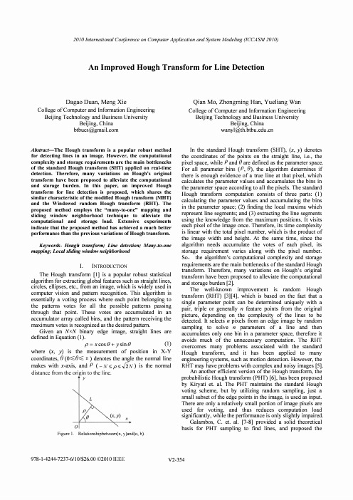
The Hough transform [1] is a popular robust statistical algorithm for extracting global features such as straight lines, circles, ellipses, etc., from an image, which is widely used in computer vision and pattern recognition. This algorithm is essentially a voting process where each point belonging to the patterns votes for all the possible patterns passing through that point. These votes are accumulated in an accumulator array called bins, and the pattern receiving the maximum votes is recognized as the desired pattern. Given an NxN binary edge image, straight lines are defined in Equation (1). (1) p x cos e + y sin e
A Fast and Accurate Plane Detection Algorithm for Large Noisy Point Clouds Using Filtered Normals
A Fast and Accurate Plane Detection Algorithm for Large Noisy Point CloudsUsing Filtered Normals and Voxel GrowingJean-Emmanuel DeschaudFranc¸ois GouletteMines ParisTech,CAOR-Centre de Robotique,Math´e matiques et Syst`e mes60Boulevard Saint-Michel75272Paris Cedex06jean-emmanuel.deschaud@mines-paristech.fr francois.goulette@mines-paristech.frAbstractWith the improvement of3D scanners,we produce point clouds with more and more points often exceeding millions of points.Then we need a fast and accurate plane detection algorithm to reduce data size.In this article,we present a fast and accurate algorithm to detect planes in unorganized point clouds usingfiltered normals and voxel growing.Our work is based on afirst step in estimating better normals at the data points,even in the presence of noise.In a second step,we compute a score of local plane in each point.Then, we select the best local seed plane and in a third step start a fast and robust region growing by voxels we call voxel growing.We have evaluated and tested our algorithm on different kinds of point cloud and compared its performance to other algorithms.1.IntroductionWith the growing availability of3D scanners,we are now able to produce large datasets with millions of points.It is necessary to reduce data size,to decrease the noise and at same time to increase the quality of the model.It is in-teresting to model planar regions of these point clouds by planes.In fact,plane detection is generally afirst step of segmentation but it can be used for many applications.It is useful in computer graphics to model the environnement with basic geometry.It is used for example in modeling to detect building facades before classification.Robots do Si-multaneous Localization and Mapping(SLAM)by detect-ing planes of the environment.In our laboratory,we wanted to detect small and large building planes in point clouds of urban environments with millions of points for modeling. As mentioned in[6],the accuracy of the plane detection is important for after-steps of the modeling pipeline.We also want to be fast to be able to process point clouds with mil-lions of points.We present a novel algorithm based on re-gion growing with improvements in normal estimation and growing process.For our method,we are generic to work on different kinds of data like point clouds fromfixed scan-ner or from Mobile Mapping Systems(MMS).We also aim at detecting building facades in urban point clouds or little planes like doors,even in very large data sets.Our input is an unorganized noisy point cloud and with only three”in-tuitive”parameters,we generate a set of connected compo-nents of planar regions.We evaluate our method as well as explain and analyse the significance of each parameter. 2.Previous WorksAlthough there are many methods of segmentation in range images like in[10]or in[3],three have been thor-oughly studied for3D point clouds:region-growing, hough-transform from[14]and Random Sample Consen-sus(RANSAC)from[9].The application of recognising structures in urban laser point clouds is frequent in literature.Bauer in[4]and Boulaassal in[5]detect facades in dense3D point cloud by a RANSAC algorithm.V osselman in[23]reviews sur-face growing and3D hough transform techniques to de-tect geometric shapes.Tarsh-Kurdi in[22]detect roof planes in3D building point cloud by comparing results on hough-transform and RANSAC algorithm.They found that RANSAC is more efficient than thefirst one.Chao Chen in[6]and Yu in[25]present algorithms of segmentation in range images for the same application of detecting planar regions in an urban scene.The method in[6]is based on a region growing algorithm in range images and merges re-sults in one labelled3D point cloud.[25]uses a method different from the three we have cited:they extract a hi-erarchical subdivision of the input image built like a graph where leaf nodes represent planar regions.There are also other methods like bayesian techniques. In[16]and[8],they obtain smoothed surface from noisy point clouds with objects modeled by probability distribu-tions and it seems possible to extend this idea to point cloud segmentation.But techniques based on bayesian statistics need to optimize global statistical model and then it is diffi-cult to process points cloud larger than one million points.We present below an analysis of the two main methods used in literature:RANSAC and region-growing.Hough-transform algorithm is too time consuming for our applica-tion.To compare the complexity of the algorithm,we take a point cloud of size N with only one plane P of size n.We suppose that we want to detect this plane P and we define n min the minimum size of the plane we want to detect.The size of a plane is the area of the plane.If the data density is uniform in the point cloud then the size of a plane can be specified by its number of points.2.1.RANSACRANSAC is an algorithm initially developped by Fis-chler and Bolles in[9]that allows thefitting of models with-out trying all possibilities.RANSAC is based on the prob-ability to detect a model using the minimal set required to estimate the model.To detect a plane with RANSAC,we choose3random points(enough to estimate a plane).We compute the plane parameters with these3points.Then a score function is used to determine how the model is good for the remaining ually,the score is the number of points belonging to the plane.With noise,a point belongs to a plane if the distance from the point to the plane is less than a parameter γ.In the end,we keep the plane with the best score.Theprobability of getting the plane in thefirst trial is p=(nN )3.Therefore the probability to get it in T trials is p=1−(1−(nN )3)ing equation1and supposing n minN1,we know the number T min of minimal trials to have a probability p t to get planes of size at least n min:T min=log(1−p t)log(1−(n minN))≈log(11−p t)(Nn min)3.(1)For each trial,we test all data points to compute the score of a plane.The RANSAC algorithm complexity lies inO(N(Nn min )3)when n minN1and T min→0whenn min→N.Then RANSAC is very efficient in detecting large planes in noisy point clouds i.e.when the ratio n minN is 1but very slow to detect small planes in large pointclouds i.e.when n minN 1.After selecting the best model,another step is to extract the largest connected component of each plane.Connnected components mean that the min-imum distance between each point of the plane and others points is smaller(for distance)than afixed parameter.Schnabel et al.[20]bring two optimizations to RANSAC:the points selection is done locally and the score function has been improved.An octree isfirst created from point cloud.Points used to estimate plane parameters are chosen locally at a random depth of the octree.The score function is also different from RANSAC:instead of testing all points for one model,they test only a random subset and find the score by interpolation.The algorithm complexity lies in O(Nr4Ndn min)where r is the number of random subsets for the score function and d is the maximum octree depth. Their algorithm improves the planes detection speed but its complexity lies in O(N2)and it becomes slow on large data sets.And again we have to extract the largest connected component of each plane.2.2.Region GrowingRegion Growing algorithms work well in range images like in[18].The principle of region growing is to start with a seed region and to grow it by neighborhood when the neighbors satisfy some conditions.In range images,we have the neighbors of each point with pixel coordinates.In case of unorganized3D data,there is no information about the neighborhood in the data structure.The most common method to compute neighbors in3D is to compute a Kd-tree to search k nearest neighbors.The creation of a Kd-tree lies in O(NlogN)and the search of k nearest neighbors of one point lies in O(logN).The advantage of these region growing methods is that they are fast when there are many planes to extract,robust to noise and extract the largest con-nected component immediately.But they only use the dis-tance from point to plane to extract planes and like we will see later,it is not accurate enough to detect correct planar regions.Rabbani et al.[19]developped a method of smooth area detection that can be used for plane detection.Theyfirst estimate the normal of each point like in[13].The point with the minimum residual starts the region growing.They test k nearest neighbors of the last point added:if the an-gle between the normal of the point and the current normal of the plane is smaller than a parameterαthen they add this point to the smooth region.With Kd-tree for k nearest neighbors,the algorithm complexity is in O(N+nlogN). The complexity seems to be low but in worst case,when nN1,example for facade detection in point clouds,the complexity becomes O(NlogN).3.Voxel Growing3.1.OverviewIn this article,we present a new algorithm adapted to large data sets of unorganized3D points and optimized to be accurate and fast.Our plane detection method works in three steps.In thefirst part,we compute a better esti-mation of the normal in each point by afiltered weighted planefitting.In a second step,we compute the score of lo-cal planarity in each point.We select the best seed point that represents a good seed plane and in the third part,we grow this seed plane by adding all points close to the plane.Thegrowing step is based on a voxel growing algorithm.The filtered normals,the score function and the voxel growing are innovative contributions of our method.As an input,we need dense point clouds related to the level of detail we want to detect.As an output,we produce connected components of planes in the point cloud.This notion of connected components is linked to the data den-sity.With our method,the connected components of planes detected are linked to the parameter d of the voxel grid.Our method has 3”intuitive”parameters :d ,area min and γ.”intuitive”because there are linked to physical mea-surements.d is the voxel size used in voxel growing and also represents the connectivity of points in detected planes.γis the maximum distance between the point of a plane and the plane model,represents the plane thickness and is linked to the point cloud noise.area min represents the minimum area of planes we want to keep.3.2.Details3.2.1Local Density of Point CloudsIn a first step,we compute the local density of point clouds like in [17].For that,we find the radius r i of the sphere containing the k nearest neighbors of point i .Then we cal-culate ρi =kπr 2i.In our experiments,we find that k =50is a good number of neighbors.It is important to know the lo-cal density because many laser point clouds are made with a fixed resolution angle scanner and are therefore not evenly distributed.We use the local density in section 3.2.3for the score calculation.3.2.2Filtered Normal EstimationNormal estimation is an important part of our algorithm.The paper [7]presents and compares three normal estima-tion methods.They conclude that the weighted plane fit-ting or WPF is the fastest and the most accurate for large point clouds.WPF is an idea of Pauly and al.in [17]that the fitting plane of a point p must take into consider-ation the nearby points more than other distant ones.The normal least square is explained in [21]and is the mini-mum of ki =1(n p ·p i +d )2.The WPF is the minimum of ki =1ωi (n p ·p i +d )2where ωi =θ( p i −p )and θ(r )=e −2r 2r2i .For solving n p ,we compute the eigenvec-tor corresponding to the smallest eigenvalue of the weightedcovariance matrix C w = ki =1ωi t (p i −b w )(p i −b w )where b w is the weighted barycenter.For the three methods ex-plained in [7],we get a good approximation of normals in smooth area but we have errors in sharp corners.In fig-ure 1,we have tested the weighted normal estimation on two planes with uniform noise and forming an angle of 90˚.We can see that the normal is not correct on the corners of the planes and in the red circle.To improve the normal calculation,that improves the plane detection especially on borders of planes,we propose a filtering process in two phases.In a first step,we com-pute the weighted normals (WPF)of each point like we de-scribed it above by minimizing ki =1ωi (n p ·p i +d )2.In a second step,we compute the filtered normal by us-ing an adaptive local neighborhood.We compute the new weighted normal with the same sum minimization but keep-ing only points of the neighborhood whose normals from the first step satisfy |n p ·n i |>cos (α).With this filtering step,we have the same results in smooth areas and better results in sharp corners.We called our normal estimation filtered weighted plane fitting(FWPF).Figure 1.Weighted normal estimation of two planes with uniform noise and with 90˚angle between them.We have tested our normal estimation by computing nor-mals on synthetic data with two planes and different angles between them and with different values of the parameter α.We can see in figure 2the mean error on normal estimation for WPF and FWPF with α=20˚,30˚,40˚and 90˚.Us-ing α=90˚is the same as not doing the filtering step.We see on Figure 2that α=20˚gives smaller error in normal estimation when angles between planes is smaller than 60˚and α=30˚gives best results when angle between planes is greater than 60˚.We have considered the value α=30˚as the best results because it gives the smaller mean error in normal estimation when angle between planes vary from 20˚to 90˚.Figure 3shows the normals of the planes with 90˚angle and better results in the red circle (normals are 90˚with the plane).3.2.3The score of local planarityIn many region growing algorithms,the criteria used for the score of the local fitting plane is the residual,like in [18]or [19],i.e.the sum of the square of distance from points to the plane.We have a different score function to estimate local planarity.For that,we first compute the neighbors N i of a point p with points i whose normals n i are close toFigure parison of mean error in normal estimation of two planes with α=20˚,30˚,40˚and 90˚(=Nofiltering).Figure 3.Filtered Weighted normal estimation of two planes with uniform noise and with 90˚angle between them (α=30˚).the normal n p .More precisely,we compute N i ={p in k neighbors of i/|n i ·n p |>cos (α)}.It is a way to keep only the points which are probably on the local plane before the least square fitting.Then,we compute the local plane fitting of point p with N i neighbors by least squares like in [21].The set N i is a subset of N i of points belonging to the plane,i.e.the points for which the distance to the local plane is smaller than the parameter γ(to consider the noise).The score s of the local plane is the area of the local plane,i.e.the number of points ”in”the plane divided by the localdensity ρi (seen in section 3.2.1):the score s =card (N i)ρi.We take into consideration the area of the local plane as the score function and not the number of points or the residual in order to be more robust to the sampling distribution.3.2.4Voxel decompositionWe use a data structure that is the core of our region growing method.It is a voxel grid that speeds up the plane detection process.V oxels are small cubes of length d that partition the point cloud space.Every point of data belongs to a voxel and a voxel contains a list of points.We use the Octree Class Template in [2]to compute an Octree of the point cloud.The leaf nodes of the graph built are voxels of size d .Once the voxel grid has been computed,we start the plane detection algorithm.3.2.5Voxel GrowingWith the estimator of local planarity,we take the point p with the best score,i.e.the point with the maximum area of local plane.We have the model parameters of this best seed plane and we start with an empty set E of points belonging to the plane.The initial point p is in a voxel v 0.All the points in the initial voxel v 0for which the distance from the seed plane is less than γare added to the set E .Then,we compute new plane parameters by least square refitting with set E .Instead of growing with k nearest neighbors,we grow with voxels.Hence we test points in 26voxel neigh-bors.This is a way to search the neighborhood in con-stant time instead of O (logN )for each neighbor like with Kd-tree.In a neighbor voxel,we add to E the points for which the distance to the current plane is smaller than γand the angle between the normal computed in each point and the normal of the plane is smaller than a parameter α:|cos (n p ,n P )|>cos (α)where n p is the normal of the point p and n P is the normal of the plane P .We have tested different values of αand we empirically found that 30˚is a good value for all point clouds.If we added at least one point in E for this voxel,we compute new plane parameters from E by least square fitting and we test its 26voxel neigh-bors.It is important to perform plane least square fitting in each voxel adding because the seed plane model is not good enough with noise to be used in all voxel growing,but only in surrounding voxels.This growing process is faster than classical region growing because we do not compute least square for each point added but only for each voxel added.The least square fitting step must be computed very fast.We use the same method as explained in [18]with incre-mental update of the barycenter b and covariance matrix C like equation 2.We know with [21]that the barycen-ter b belongs to the least square plane and that the normal of the least square plane n P is the eigenvector of the smallest eigenvalue of C .b0=03x1C0=03x3.b n+1=1n+1(nb n+p n+1).C n+1=C n+nn+1t(pn+1−b n)(p n+1−b n).(2)where C n is the covariance matrix of a set of n points,b n is the barycenter vector of a set of n points and p n+1is the (n+1)point vector added to the set.This voxel growing method leads to a connected com-ponent set E because the points have been added by con-nected voxels.In our case,the minimum distance between one point and E is less than parameter d of our voxel grid. That is why the parameter d also represents the connectivity of points in detected planes.3.2.6Plane DetectionTo get all planes with an area of at least area min in the point cloud,we repeat these steps(best local seed plane choice and voxel growing)with all points by descending order of their score.Once we have a set E,whose area is bigger than area min,we keep it and classify all points in E.4.Results and Discussion4.1.Benchmark analysisTo test the improvements of our method,we have em-ployed the comparative framework of[12]based on range images.For that,we have converted all images into3D point clouds.All Point Clouds created have260k points. After our segmentation,we project labelled points on a seg-mented image and compare with the ground truth image. We have chosen our three parameters d,area min andγby optimizing the result of the10perceptron training image segmentation(the perceptron is portable scanner that pro-duces a range image of its environment).Bests results have been obtained with area min=200,γ=5and d=8 (units are not provided in the benchmark).We show the re-sults of the30perceptron images segmentation in table1. GT Regions are the mean number of ground truth planes over the30ground truth range images.Correct detection, over-segmentation,under-segmentation,missed and noise are the mean number of correct,over,under,missed and noised planes detected by methods.The tolerance80%is the minimum percentage of points we must have detected comparing to the ground truth to have a correct detection. More details are in[12].UE is a method from[12],UFPR is a method from[10]. It is important to notice that UE and UFPR are range image methods and our method is not well suited for range images but3D Point Cloud.Nevertheless,it is a good benchmark for comparison and we see in table1that the accuracy of our method is very close to the state of the art in range image segmentation.To evaluate the different improvements of our algorithm, we have tested different variants of our method.We have tested our method without normals(only with distance from points to plane),without voxel growing(with a classical region growing by k neighbors),without our FWPF nor-mal estimation(with WPF normal estimation),without our score function(with residual score function).The compari-son is visible on table2.We can see the difference of time computing between region growing and voxel growing.We have tested our algorithm with and without normals and we found that the accuracy cannot be achieved whithout normal computation.There is also a big difference in the correct de-tection between WPF and our FWPF normal estimation as we can see in thefigure4.Our FWPF normal brings a real improvement in border estimation of planes.Black points in thefigure are non classifiedpoints.Figure5.Correct Detection of our segmentation algorithm when the voxel size d changes.We would like to discuss the influence of parameters on our algorithm.We have three parameters:area min,which represents the minimum area of the plane we want to keep,γ,which represents the thickness of the plane(it is gener-aly closely tied to the noise in the point cloud and espe-cially the standard deviationσof the noise)and d,which is the minimum distance from a point to the rest of the plane. These three parameters depend on the point cloud features and the desired segmentation.For example,if we have a lot of noise,we must choose a highγvalue.If we want to detect only large planes,we set a large area min value.We also focus our analysis on the robustess of the voxel size d in our algorithm,i.e.the ratio of points vs voxels.We can see infigure5the variation of the correct detection when we change the value of d.The method seems to be robust when d is between4and10but the quality decreases when d is over10.It is due to the fact that for a large voxel size d,some planes from different objects are merged into one plane.GT Regions Correct Over-Under-Missed Noise Duration(in s)detection segmentation segmentationUE14.610.00.20.3 3.8 2.1-UFPR14.611.00.30.1 3.0 2.5-Our method14.610.90.20.1 3.30.7308Table1.Average results of different segmenters at80%compare tolerance.GT Regions Correct Over-Under-Missed Noise Duration(in s) Our method detection segmentation segmentationwithout normals14.6 5.670.10.19.4 6.570 without voxel growing14.610.70.20.1 3.40.8605 without FWPF14.69.30.20.1 5.0 1.9195 without our score function14.610.30.20.1 3.9 1.2308 with all improvements14.610.90.20.1 3.30.7308 Table2.Average results of variants of our segmenter at80%compare tolerance.4.1.1Large scale dataWe have tested our method on different kinds of data.We have segmented urban data infigure6from our Mobile Mapping System(MMS)described in[11].The mobile sys-tem generates10k pts/s with a density of50pts/m2and very noisy data(σ=0.3m).For this point cloud,we want to de-tect building facades.We have chosen area min=10m2, d=1m to have large connected components andγ=0.3m to cope with the noise.We have tested our method on point cloud from the Trim-ble VX scanner infigure7.It is a point cloud of size40k points with only20pts/m2with less noise because it is a fixed scanner(σ=0.2m).In that case,we also wanted to detect building facades and keep the same parameters ex-ceptγ=0.2m because we had less noise.We see infig-ure7that we have detected two facades.By setting a larger voxel size d value like d=10m,we detect only one plane. We choose d like area min andγaccording to the desired segmentation and to the level of detail we want to extract from the point cloud.We also tested our algorithm on the point cloud from the LEICA Cyrax scanner infigure8.This point cloud has been taken from AIM@SHAPE repository[1].It is a very dense point cloud from multiplefixed position of scanner with about400pts/m2and very little noise(σ=0.02m). In this case,we wanted to detect all the little planes to model the church in planar regions.That is why we have chosen d=0.2m,area min=1m2andγ=0.02m.Infigures6,7and8,we have,on the left,input point cloud and on the right,we only keep points detected in a plane(planes are in random colors).The red points in thesefigures are seed plane points.We can see in thesefig-ures that planes are very well detected even with high noise. Table3show the information on point clouds,results with number of planes detected and duration of the algorithm.The time includes the computation of the FWPF normalsof the point cloud.We can see in table3that our algo-rithm performs linearly in time with respect to the numberof points.The choice of parameters will have little influence on time computing.The computation time is about one mil-lisecond per point whatever the size of the point cloud(we used a PC with QuadCore Q9300and2Go of RAM).The algorithm has been implented using only one thread andin-core processing.Our goal is to compare the improve-ment of plane detection between classical region growing and our region growing with better normals for more ac-curate planes and voxel growing for faster detection.Our method seems to be compatible with out-of-core implemen-tation like described in[24]or in[15].MMS Street VX Street Church Size(points)398k42k7.6MMean Density50pts/m220pts/m2400pts/m2 Number of Planes202142Total Duration452s33s6900sTime/point 1ms 1ms 1msTable3.Results on different data.5.ConclusionIn this article,we have proposed a new method of plane detection that is fast and accurate even in presence of noise. We demonstrate its efficiency with different kinds of data and its speed in large data sets with millions of points.Our voxel growing method has a complexity of O(N)and it is able to detect large and small planes in very large data sets and can extract them directly in connected components.Figure 4.Ground truth,Our Segmentation without and with filterednormals.Figure 6.Planes detection in street point cloud generated by MMS (d =1m,area min =10m 2,γ=0.3m ).References[1]Aim@shape repository /.6[2]Octree class template /code/octree.html.4[3] A.Bab-Hadiashar and N.Gheissari.Range image segmen-tation using surface selection criterion.2006.IEEE Trans-actions on Image Processing.1[4]J.Bauer,K.Karner,K.Schindler,A.Klaus,and C.Zach.Segmentation of building models from dense 3d point-clouds.2003.Workshop of the Austrian Association for Pattern Recognition.1[5]H.Boulaassal,ndes,P.Grussenmeyer,and F.Tarsha-Kurdi.Automatic segmentation of building facades using terrestrial laser data.2007.ISPRS Workshop on Laser Scan-ning.1[6] C.C.Chen and I.Stamos.Range image segmentationfor modeling and object detection in urban scenes.2007.3DIM2007.1[7]T.K.Dey,G.Li,and J.Sun.Normal estimation for pointclouds:A comparison study for a voronoi based method.2005.Eurographics on Symposium on Point-Based Graph-ics.3[8]J.R.Diebel,S.Thrun,and M.Brunig.A bayesian methodfor probable surface reconstruction and decimation.2006.ACM Transactions on Graphics (TOG).1[9]M.A.Fischler and R.C.Bolles.Random sample consen-sus:A paradigm for model fitting with applications to image analysis and automated munications of the ACM.1,2[10]P.F.U.Gotardo,O.R.P.Bellon,and L.Silva.Range imagesegmentation by surface extraction using an improved robust estimator.2003.Proceedings of Computer Vision and Pat-tern Recognition.1,5[11] F.Goulette,F.Nashashibi,I.Abuhadrous,S.Ammoun,andurgeau.An integrated on-board laser range sensing sys-tem for on-the-way city and road modelling.2007.Interna-tional Archives of the Photogrammetry,Remote Sensing and Spacial Information Sciences.6[12] A.Hoover,G.Jean-Baptiste,and al.An experimental com-parison of range image segmentation algorithms.1996.IEEE Transactions on Pattern Analysis and Machine Intelligence.5[13]H.Hoppe,T.DeRose,T.Duchamp,J.McDonald,andW.Stuetzle.Surface reconstruction from unorganized points.1992.International Conference on Computer Graphics and Interactive Techniques.2[14]P.Hough.Method and means for recognizing complex pat-terns.1962.In US Patent.1[15]M.Isenburg,P.Lindstrom,S.Gumhold,and J.Snoeyink.Large mesh simplification using processing sequences.2003.。
- 1、下载文档前请自行甄别文档内容的完整性,平台不提供额外的编辑、内容补充、找答案等附加服务。
- 2、"仅部分预览"的文档,不可在线预览部分如存在完整性等问题,可反馈申请退款(可完整预览的文档不适用该条件!)。
- 3、如文档侵犯您的权益,请联系客服反馈,我们会尽快为您处理(人工客服工作时间:9:00-18:30)。
A Robust Decision Tree Algorithm for Imbalanced Data SetsWei Liu∗Sanjay Chawla∗David A.Cieslak†Nitesh V.Chawla†AbstractWe propose a new decision tree algorithm,Class Confidence Proportion Decision Tree(CCPDT),which is robust and insensitive to size of classes and generates rules which are statistically significant.In order to make decision trees robust,we begin by expressing Information Gain,the metric used in C4.5,in terms of confidence of a rule.This allows us to immediately explain why Information Gain,like confidence,results in rules which are biased towards the majority class.To overcome this bias,we introduce a new measure,Class Confidence Proportion(CCP),which forms the basis of CCPDT.To generate rules which are statistically significant we design a novel and efficient top-down and bottom-up approach which uses Fisher’s exact test to prune branches of the tree which are not statistically significant.Together these two changes yield a classifier that performs statistically better than not only traditional decision trees but also trees learned from data that has been balanced by well known sampling techniques.Our claims are confirmed through extensive experiments and comparisons against C4.5,CART, HDDT and SPARCCC.1IntroductionWhile there are several types of classifiers,rule-based classi-fiers have the distinct advantage of being easily interpretable. This is especially true in a“data mining”setting,where the high dimensionality of data often means that apriori very lit-tle is known about the underlying mechanism which gener-ated the data.Decision trees are perhaps the most popular form of rule-based classifiers(such as the well-known C4.5[15]). Recently however,classifiers based on association rules have also become popular[19]which are often called associa-tive classifiers.Associative classifiers use association rule mining to discover interesting and significant rules from the training data,and the set of rules discovered constitute the classifier.The canonical example of an associative classi-fier is CBA(classification based on associations)[14],which ∗Centre for Distributed and High Performance Computing,School of Information Technologies,the University of Sydney,Sydney NSW2006, Australia.{weiliu,chawla}@.au†University of Notre Dame,Notre Dame IN46556,USA.dcies-lak@,nchawla@ uses the minimum support and confidence framework tofind rules.The accuracy of associative classifiers depends on the quality of their discovered rules.However,the success of both decision trees and associate classifiers depends on the assumption that there is an equal amount of information for each class contained in the training data.In binary classifi-cation problems,if there is a similar number of instances for both positive and negative classes,both C4.5and CBA gen-erally perform well.On the other hand,if the training data set tends to have an imbalanced class distribution,both types of classifier will have a bias towards the majority class.As it happens,an accurate prediction is typically related to the minority class–the class that is usually of greater interest.One way of solving the imbalance class problem is to modify the class distributions in the training data by over-sampling the minority class or under-sampling the majority class.For instance,SMOTE[5]uses over-sampling to increase the number of the minority class instances,by creating synthetic samples.Further variations on SMOTE [7]have integrated boosting with sampling strategies to better model the minority class,by focusing on difficult samples that belong to both minority and majority classes.Nonetheless,data sampling is not the only way to deal with class imbalanced problems:some specifically designed “imbalanced data oriented”algorithms can perform well on the original unmodified imbalanced data sets.For example, a variation on associative classifier called SPARCCC[19] has been shown to outperform CBA[14]and CMAR[13]on imbalanced data sets.The downside of SPARCCC is that it generates a large number of rules.This seems to be a feature of all associative classifiers and negates many of the advantages of rule-based classification.In[8],the Hellinger distance(HDDT)was used as the decision tree splitting criterion and shown to be insensitive towards class distribution skewness.We will compare and discuss CCPDT and HDDT more extensively in Section3.4. Here it will be suffice to state that while HDDT is based on likelihood difference,CCPDT is based on likelihood ratio.In order to prevent trees from over-fitting the data, all decision trees use some form of pruning.Traditional pruning algorithms are based on error estimations-a node is pruned if the predicted error rate is decreased.But this pruning technique will not always perform well on imbalanced data sets.[4]has shown that pruning in C4.5can have a detrimental effect on learning from imbalanced datasets,since lower error rates can be achieved by removing the branches that lead to minority class leaves.In contrast our pruning is based on Fisher’s exact test,which checks if a path in a decision tree is statistically significant;and if not,the path will be pruned.As an added advantage,every resulting tree path(rule)will also be statistically significant.Main Insight The main insight of the paper can be summa-rized as follows.Let X be an attribute and y a class.Let X→y and¬X→y be two rules,with confidence p and q respectively.Then we can express Information Gain(IG)in terms of the two confidences.Abstractly,IG C4.5=F(p,q)where F is an abstract function.We will show that a splitting measure based on confidence will be biased towards the majority class.Our innovation is to use Class Confidence Proportion(CCP)instead of confidence.Abstractly CCP of the X→y and¬X→y is r and s.We define a new splitting criterionIG CCP DT=F (r,s)The main thrust in the paper is to show that IG CCP DT1 is more robust to class imbalance than IG C4.5and behave similarly when the classes are balanced.The approach of replacing a conventional splitting mea-sure by CCP is a generic mechanism for all traditional deci-sion trees that are based on the“balanced data”assumption. It can be applied to any decision tree algorithm that checks the degree of impurity inside a partitioned branch,such as C4.5and CART etc.The rest of the paper is structured as follows.In Section 2,we analyze the factors that causes CBA and C4.5perform poorly on imbalanced data sets.In Section3,we introduce CCP as the measure of splitting attributes during decision tree construction.In Section4we present a full decision tree algorithm which details how we incorporate CCP and use Fisher’s Exact Test(FET)for pruning.A wrapper framework utilizing sampling techniques is introduced in Section5. Experiments,Results and Analysis are presented in Section 6.We conclude in Section7with directions for research.2Rule-based ClassifiersWe analyze the metrics used by rule-based classifiers in the context of imbalanced data.Wefirst show that the ranking of rules based on confidence is biased towards the majority class,and then express information gain and Gini index as functions of confidence and show that they also suffer from similar problems.1IG CCP DT is not Information Gain which has a specific meaning.Table1:An example of notations for CBA analysisX¬XΣInstancesy a b a+b¬y c d c+dΣAttributes a+c b+d n2.1CBA The performance of Associative Classifiers de-pends on the quality of the rules it discovers during the train-ing process.We now demonstrate that in an imbalanced set-ting,confidence is biased towards the majority class.Suppose we have a training data set which consists of n records,and the antecedents(denoted by X and¬X)and class(y and¬y)distributions are in the form of Table1. The rule selection strategy in CBA is tofind all rule items that have support and confidence above some predefined thresholds.For a rule X→y,its confidence is defined as:(2.1)Conf(X→y)=Supp(X∪y)Supp(X)=aa+c“Conf”and“Supp”stand for Confidence and Support. Similarly,we have:(2.2)Conf(X→¬y)=Supp(X∪¬y)Supp(X)=ca+c Equation2.1suggests that selecting the highest confi-dence rules means choosing the most frequent class among all the instances that contains that antecedent(i.e.X in this example).However,for imbalanced data sets,since the size of the positive class is always much smaller than the nega-tive class,we always have:a+b c+d(suppose y is the positive class).Given that imbalanced data do not affect the distribution of antecedents,we can,without loss of general-ity,assume that X s and¬X s are nearly equally distributed. Hence when data is imbalanced,a and b are both small while c and d are both large.Even if y is supposed to occur with X more frequently than¬y,c is unlikely to be less than a because the positive class size will be much smaller than the negative class size.Thus,it is not surprising that the right-side term in Equation2.2always tends to be lower bounded by the right-side term in Equation2.1.It appears that even though the rule X→¬y may not be significant,it is easy for it to have a high confidence value.In these circumstances,it is very hard for the confidence of a“good”rule X→y to be significantly larger than that of a“bad”rule X→¬y.What is more,because of its low confidence,during the classifier building process a“good”rule may be ranked behind some other rules just because they have a higher confidence because they predict the majority class.This is a fatal error,since in an imbalanced class problem it is often the minority class that is of more interest.2.2Traditional decision trees Decision trees such as C4.5use information gain to decide which variable to split [15].The information gain from splitting a node t is defined as:(2.3)InfoGain split =Entropy (t )−i =1,2n in Entropy (i )where i represents one of the sub-nodes after splitting(assume there are 2sub-nodes),n i is the number of instances in subnote i ,and n stands for the total number of instances.In binary-class classification,the entropy of node t is defined as:(2.4)Entropy (t )=−j =1,2p (j |t )log p (j |t )where j represents one of the two classes.For a fixed training set (or its subsets),the first term in Equation 2.3is fixed,because the number of instances for each class (i.e.p (j |t )in equation 2.4)is the same for all attributes.To this end,the challenge of maximizing information gain in Equation 2.3reduces to maximizing the second term − i =1,2n in Entropy (i ).If the node t is split into two subnodes with two corre-sponding paths:X and ¬X ,and the instances in each node have two classes denoted by y and ¬y ,Equation 2.3can be rewritten as:InfoGain split =Entropy (t )−n 1n [−p (y |X )log(y |X )−p (¬y |X )log p (¬y |X )]−n 2n[−p (y |¬X )log(y |¬X )−p (¬y |¬X )log p (¬y |¬X )](2.5)Note that the probability of y given X is equivalent to the confidence of X →y :(2.6)p (y |X )=p (X ∩y )=Support (X ∪y )=Conf (X →y )Then if we denote Conf (X →y )by p ,and denoteConf (¬X →y )by q (hence Conf (X →¬y )=1−p and Conf (¬X →¬y )=1−q ),and ignore the “fixed”terms Entropy(t)in equation 2.5,we can obtain the relationship in Equation 2.7.The first approximation step in Equation 2.7ignores the first term Entropy(t),then the second approximation transforms the addition of logarithms to multiplications.Based on Equation 2.7the distribution of information gain as a function of Conf (X →y )and Conf (¬X →y )is shown in Figure rmation gain is maximized when Conf (X →y )and Conf (¬X →y )are both closeto Figure 1:Approximation of information gain in the formula formed by Conf (X →y )and Conf (¬X →y )from Equa-tion rmation gain is the lowest when Conf (X →y )and Conf (¬X →y )are both close to 0.5,and is the highest when both Conf (X →y )and Conf (¬X →y )reaches 1or 0.either 0or 1,and is minimized when Conf (X →y )andConf (¬X →y )are both close to 0.5.Note that when Conf (X →y )is close to 0,Conf (X →¬y )is close to 1;when Conf (¬X →y )is close to 0,Conf (¬X →¬y )is close to 1.Therefore,information gain achieves the highestvalue when either X →y or X →¬y has the highest confidence,and either ¬X →y or ¬X →¬y also has the highest confidence.InfoGain split =Entropy (t )+ i =1,2n in Entropy (i )=Entropy (t )+n 1[p log p +(1−p )log(1−p )]+n 2n[q log q +(1−q )log(1−q )]∝n 1[p log p +(1−p )log(1−p )]+n 2n[q log q +(1−q )log(1−q )]∝n 1n log p p (1−p )1−p +n 2nlog q q (1−q )1−q(2.7)Therefore,decision trees such as C4.5split an attribute whose partition provides the highest confidence.This strat-egy is very similar to the rule-ranking mechanism of asso-ciation classifiers.As we have analyzed in Section 2.1,for imbalanced data set,high confidence rules do not necessarily imply high significance in imbalanced data,and some signif-icant rules may not yield high confidence.Thus we can assert that the splitting criteria in C4.5is suitable for balanced but not imbalanced data sets.We note that it is the term p (j |t )in Equation 2.4that is the cause of the poor behavior of C4.5in imbalanced situations.However,p (j |t )also appears in other decisionTable2:Confusion Matrix for the classification of two classesAll instances Predicted positive Predicted negativeActual positive true positive(tp)false negative(fn)Actual negative false positive(fp)true negative(tn) tree measures.For example,the Gini index defined in CART [2]can be expressed as:(2.8)Gini(t)=1−jp(j|t)2Thus decision tree based on CART will too suffer from the imbalanced class problem.We now propose another measure which will be more robust in the imbalanced data situation. 3Class Confidence Proportion and Fisher’s Exact Test Having identified the weakness of the support-confidence framework and the factor that results in the poor performance of entropy and Gini index,we are now in a position to propose new measures to address the problem.3.1Class Confidence Proportion As previously ex-plained,the high frequency with which a particular class y appears together with X does not necessarily mean that X “explains”the class y,because y could be the overwhelming majority class.In such cases,it is reasonable that instead of focusing on the antecedents(X s),we focus only on each class andfind the most significant antecedents associated with that class.In this way,all instances are partitioned ac-cording to the class they contain,and consequently instances that belong to different classes will not have an impact on each other.To this end,we define a new concept,Class Con-fidence(CC),tofind the most interesting antecedents(X s) from all the classes(y s):(3.9)CC(X→y)=Supp(X∪y)The main difference between this CC and traditional confidence is the denominator:we use Supp(y)instead of Supp(X)so as to focus only on each class.In the notation of the confusion matrix(Table2)CC can be expressed as:(3.10)CC(X→y)=T rueP ositiveInstancesActualP ositiveInstances=tptp+fn(3.11)CC(X→¬y)=F alseP ositiveInstancesActualNegativeInstances=fpfp+tnWhile traditional confidence examines how many predicted positive/negative instances are actually posi-(a)Classes are balanced(b)Classes are imbalanced(1:10) Figure2:Information gain from original entropy when a data set follows different class pared with the contour lines in(a),those in(b)shift towards the top-left and bottom-right.tive/negative(the precision),CC is focused in how many ac-tual positive/negative instances are predicted correctly(the recall).Thus,even if there are many more negative than pos-itive instances in the data set(tp+fn fp+tn),Equations 3.10and3.11will not be affected by this imbalance.Con-sequently,rules with high CC will be the significant ones, regardless of whether they are discovered from balanced or imbalanced data sets.However,obtaining high CC rules is still insufficient for solving classification problems–it is necessary to ensure that the classes implied by those rules are not only of high confidence,but more interesting than their corresponding alternative classes.Therefore,we propose the proportion of one CC over that of all classes as our measure of how interesting the class is–what we call the CC Proportion (CCP).The CCP of rule X→y is defined as:CCP(X→y)=CC(X→y)(3.12)A rule with high CCP means that,compared with its alternative class,the class this rule implies has higher CC, and consequently is more likely to occur together with this rule’s antecedents regardless of the proportion of classes in the data set.Another benefit of taking this proportion is the ability to scale CCP between[0,1],which makes it possible to replace the traditional frequency term in entropy (the factor p(j|t)in Equation2.4)by CCP.Details of the CCP replacement in entropy is introduced in Section4. 3.2Robustness of CCP We now evaluate the robustness of CCP using ROC-based isometric plots proposed in Flach [10]and which are inherently independent of class and misclassification costs.The2D ROC space is spanned by false positive rate (x-axis)and the true positive rate(y-axis).The contours mark out the lines of constant value,of the splitting criterion,conditioned on the imbalanced class ratio.Metrics which are robust to class imbalance should have similar contour plots for different class ratios.In Figure2,the contour plots of information gain are shown for class ratios of1:1and1:10,respectively.It is clear,from the twofigures,that when the class distributions become more imbalanced,the contours tend to beflatter and further away from the diagonal.Thus,given the same true positive rate and false positive rate,information gain for imbalanced data sets(Figure2b)will be much lower than for balanced data sets(Figure2a).Following the model of relative impurity proposed Flach in[10],we now derive the definition for the CCP Impurity Measure.Equation3.12gives:(3.13)CCP(X→y)=tptptp+fn+fpfp+tn=tprtpr+fprwhere tpr/fpr represents true/false positive rate.For each node-split in tree construction,at least two paths will be generated,if one is X→y,the other one will be¬X→¬y with CCP:(3.14)CCP(¬X→¬y)=tnfp+tntn+fn=1−fpr2−tpr−fprThe relative impurity for C4.5proposed in[10]is: InfoGain C4.5=Imp(tp+fn,fp+tn)−(tp+fp)∗Imp(tptp+fp,fptp+fp)−(fn+tn)∗Imp(fnfn+tn,tnfn+tn)(3.15)where Imp(p,n)=-p log p-n log n.Thefirst term in the right side represents the entropy of the node before splitting, while the sum of the second and third terms represents the entropy of the two subnodes after splitting.Take thesecond term(tp+fp)∗Imp(tptp+fp ,fptp+fp)as an example,thefirst frequency measure tptp+fp is an alternative way ofinterpreting the confidence of rule X→y;similarly,thesecond frequency measure fptp+fp is equal to the confidenceof rule X→¬y.We showed in Section2.2that both terms are inappropriate for imbalanced data learning.To overcome the inherent weakness in traditional deci-sion trees,we apply CCP into this impurity measure and thus rewrite the information gain definition in Equation3.15as the CCP Impurity Measure:(a)Classes arebalanced(b)Classes are imbalanced(1:10) Figure3:Information gain from CCP-embedded entropy when a data set follows different class distributions.No contour line shifts when data sets becomes imbalanced.InfoGain CCP=Imp(tp+fn,fp+tn)−(tpr+fpr)∗Imp(tprtpr+fpr,fprtpr+fpr)−(2−tpr−fpr)∗Imp(1−tpr,1−fpr) (3.16)where Imp(p,n)is still“-p log p-n log n”,while the origi-nal frequency term is replaced by CCP.The new isometric plots,with the CCP replacement,are presented in Figure3(a,b).A comparison of the twofigures tells that contour lines remain unchanged,demonstrating that CCP is unaffected by the changes in the class ratio.3.3Properties of CCP If all instances contained in a node belong to the same class,its entropy is minimized (zero).The entropy is maximized when a node contains equal number of elements from both classes.By taking all possible combinations of elements in the confusion matrix(Table2),we can plot the entropy surface as a function of tpr and fpr as shown in Figure4.Entropy (Figure4a)is the highest when tpr and fpr are equal,since “tpr=fpr”in subnodes is equivalent to elements in the subnodes being equally split between the two classes.On the other hand,the larger the difference between tpr and fpr,the purer the subnodes and the smaller their entropy.However, as stated in Section3.2,when data sets are imbalanced,the pattern of traditional entropy will become distorted(Figure 4b).Since CCP-embedded“entropy”is insensitive to class skewness,its will always exhibit afixed pattern,and this pattern is the same as traditional entropy’s balanced data situation.This can be formalized as follows:By using the notations in the confusion matrix,the fre-quency term in traditional entropy is p traditional=tptp+fp,while in CCP-based entropy it is p CCP=tprtpr+fpr.When classes in a data set are evenly distributed,we have tp+fn=(a)Traditional entropy on balanced datasets(b)Traditional entropy on imbalanced data sets.(Positive:Negative=1:10)(c)CCP-embedded entropy on any data setsFigure4:The sum of subnodes’entropy after splitting.When a data set is imbalanced,the entropy surf(b)is“distored”from(a);but for CCP-embedded“entropy”(c),the surface is always the same independent of the imbalance in the data.fp+tn,and by applying it in the definition of CCP we obtain:p CCP=tprtpr+fpr=tptp+fntptp+fn+fpfp+tn=tptp+fp=p traditionalThus when there are same number of instances in each class,the patterns of CCP-embedded entropy and traditional entropy will be the same.More importantly,this pattern is preserved for CCP-embedded entropy independent of the imbalance the data sets.This is confirmed in Figure4c which is always similar to the pattern of Figure4a regardless of the class distributions.3.4Hellinger Distance and its relationship with CCP The divergence of two absolutely continuous distributions can be measured by Hellinger distance with respect to the parameterλ[17,11],in the form of:d H(P,Q)=Ω(√−)2dλIn the Hellinger distance based decision tree(HDDT) technique[8],the distribution P and Q are assumed to be the normalized frequencies of feature values(“X”in our notation)across classes.The Hellinger distance is used to capture the propensity of a feature to separate the classes.In the tree-construction algorithm in HDDT,a feature is selected as a splitting attribute when it produces the largest Hellinger distance between the two classes.This distance is essentially captured in the differences in the relative frequencies of the attribute values for the two classes, respectively.The following formula,derived in[8],relates HDDT with the true positive rate(tpr)and false positive rate(fpr).(3.17)Impurity HD=(tpr−fpr)2+(1−tpr−1−fpr)2Figure5:The attribute selection mechanisms of CCP andHellinger distances.This example illustrates a complemen-tary situation where,while Hellinger distance can only pri-oritizes B and C,CCP distinguishes only A and B.This was also shown to be insensitive to class distribu-tions in[8],since the only two variables in this formula aretpr and fpr,without the dominating class priors.Like the Hellinger distance,CCP is also just based ontpr and fpr as shown in Equation3.13.However,there is asignificant difference between CCP and Hellinger distance.While Hellinger distance take the square root difference oftpr and fpr(|√tpr−√fpr|)as the divergence of one classdistribution from the other,CCP takes the proportion of tprand fpr as a measurement of interest.A graphical differencebetween the two measures is shown in Figure5.If we draw a straight line(Line3)parallel to the diagonalin Figure5,the segment length from origin to cross-pointbetween Line3and the y-axis is|tpr o−fpr o|(tpr oand fpr o can be the coordinates of any point in Line3),isproportional to the Hellinger distance(|√tpr−√fpr|).From this point of view,HDDT selects the point on those parallel lines with the longest segment.Therefore,in Figure 5,all the points in Line 3have a larger Hellinger distance than those in Line 4;thus points in Line 3will have higher priority in the selection of attributes.As CCP =tpr tpr +fprcan be rewritten as tpr =CCP1−CCP fpr ,CCP is proportional to the the slope of the line formed by the data point and the origin,and consequently favors the line with the highest slope.In Figure 5,the points in Line 1are considered by CCP as better splitting attributes than those in Line 2.By analyzing CCP and Hellinger distances in terms of lines in a tpr versus fpr reference frame,we note that CCP and Hellinger distance share a common problem.We give an example as follows.Suppose we have three points,A (fpr A ,tpr A ),B (fpr B ,tpr B )and C (fpr C ,tpr C ),where A is one Line 1and 3,B on Line 2and 3,and C on Line 2and 4(shown in Figure 5).Then A and B are on the same line (Line 3)that is parallel to the diagonal (i.e.|fpr A −tpr A |=|fpr B −tpr B |),while B and C are on the same line (Line 2)passing through the origin(i.e.tpr Bfpr B =tpr C fpr C).Hellinger distances will treat A and B as better splitting attributes than C,because as explained above all points in Line 3has longer Hellinger distances than Line 4.By contrast,CCP will consider A has higher splitting priorities than both B and C,since all points in Line 1obtains greater CCP than Line 2.However,on points in Line 3such as A and B,Hellinger distance fails to distinguish them ,since they will generate the same tpr vs.fpr difference.In this circumstance,HDDT may make an noneffective decision in attribute selection.This problem will become significant when the number of attributes is large,and many attributeshave similar |tpr −fpr |(or more precisely |√tpr −√fpr |)difference.The same problem occurs in the CCP measurement on testing points in Line 2such as B against C.Our solution to this problem is straightforward:when choosing the splitting attribute in decision tree construction,we select the one with the highest CCP by default,and if there are attributes that possess similar CCP values,we prioritize them on the basis of their Hellinger distances.Thus,in Figure 5,the priority of the three points will be A >B >C ,since Point A has a greater CCP value than Points B and C,and Point B has higher Hellinger distance than Point C.Details of these attribute-selecting algorithms are in Section 4.3.5Fisher’s Exact Test While CCP helps to select which branch of a tree are “good”to discriminate between classes,we also want to evaluate the statistical significance of each branch.This is done by the Fisher’s exact test (FET).For a rule X →y ,the FET will find the probability of obtaining the contingency table where X and y are more positively associated,under the null hypothesis that {X,¬X }and{y,¬y }are independent [19].The p value of this rule is given by:(3.18)p ([a,b ;c,d ])=min (b,c )i =0(a +b )!(c +d )!(a +c )!(b +d )!n !(a +i )!(b −i )!(c −i )!(d +i )!During implementation,the factorials in the p -value def-inition can be handled by expressing their values logarithmi-cally.A low p value means that the variable independence null hypothesis is rejected (no relationship between X and y );in other words,there is a positive association between the upper-left cell in the contingency table (true positives)and the lower-right (true negatives).Therefore,given a threshold for the p value,we can find and keep the tree branches that are statistically significant (with lower p values),and discard those tree nodes that are not.4CCP-based decision trees (CCPDT)In this section we provide details of the CCPDT algorithm.We modify the C4.5splitting criterion based on entropy and replace the frequency term by CCP.Due to space limits,we omit the algorithms for CCP-embedded CART,but the approach is identical to C4.5(in that the same factor is replaced with CCP).Algorithm 1(CCP-C4.5)Creation of CCP-based C4.5Input:Training Data:T D Output:Decision Tree1:if All instances are in the same class then 2:Return decision tree with one node (root),labeled as theinstances’class,3:else 4://Find the best splitting attribute (Attri ),5:Attri =MaxCCPGain(T D ),6:Assign Attri to the tree root (root =Attri ),7:for each value v i of Attri do 8:Add a branch for v i ,9:if No instance is v i at attribute Attri then 10:Add a leaf to this branch.11:else 12:Add a subtree CCP −C 4.5(T D v i )to this branch,13:end if 14:end for 15:end if4.1Build tree The original definition of entropy in deci-sion trees is presented in Equation 2.4.As explained in Sec-tion 2.2,the factor p (j |t )in Equation 2.4is not a good crite-rion for learning from imbalanced data sets,so we replace it with CCP and define the CCP-embedded entropy as:。