W6B 数据变换
多维小波变换工具箱

多维小波变换工具箱Multi-dimension Wavelet ToolboxVersion 1.0作者:陈甫一、函数的简要说明convnd 对多维数据在某一维向上做线性卷积convndcut 和convnd差不多,但加上了可以截取卷积结果的中间一部分而把两边删去的功能dyaddownnd 隔点采样dyadupnd 在两点间添0dwtnd1 多维空间中一个维向上的一次小波变换dwtndn 多维空间一次小波变换(各维向都做一次)wavedecnd 多维空间多次小波变换分解idwtnd1 多维空间中一个维向上的一次小波逆变换idwtndn 多维空间一次小波逆变换waverecnd 多维空间多次小波逆变换重构packup 利用dwtndn和wavedecnd的结果拼成多维系数空间的表示形式fitscale 改变数据值的分布以利于图像显示show3d 用图像显示三维空间的小波变换系数二、实例实例一 dwtnd1和idwtnd1r=rand(4,4,4) %随机生成一个多维空间的数据,这里是个4*4*4的三维空间r(:,:,1) =0.2028 0.1988 0.9318 0.52520.1987 0.0153 0.4660 0.20260.6038 0.7468 0.4186 0.67210.2722 0.4451 0.8462 0.8381r(:,:,2) =0.0196 0.5028 0.1897 0.54170.6813 0.7095 0.1934 0.15090.3795 0.4289 0.6822 0.69790.8318 0.3046 0.3028 0.3784r(:,:,3) =0.8600 0.8998 0.6602 0.53410.8537 0.8216 0.3420 0.72710.5936 0.6449 0.2897 0.30930.4966 0.8180 0.3412 0.8385r(:,:,4) =0.5681 0.4449 0.9568 0.97970.3704 0.6946 0.5226 0.27140.7027 0.6213 0.8801 0.25230.5466 0.7948 0.1730 0.8757[ca,cd]=dwtnd1(r,1,'haar') %对数据r在第一维向即row方向做一次haar小波分解ca(:,:,1) =0.2839 0.1514 0.9884 0.51460.6194 0.8428 0.8944 1.0679ca(:,:,2) =0.4956 0.8572 0.2709 0.48970.8565 0.5187 0.6965 0.7610ca(:,:,3) =1.2117 1.2172 0.7087 0.89180.7708 1.0344 0.4461 0.8116ca(:,:,4) =0.6636 0.8057 1.0461 0.88470.8834 1.0014 0.7447 0.7977cd(:,:,1) =0.0029 0.1298 0.3294 0.22800.2345 0.2133 -0.3023 -0.1174cd(:,:,2) =-0.4678 -0.1461 -0.0027 0.2763-0.3198 0.0879 0.2683 0.2259cd(:,:,3) =0.0045 0.0553 0.2250 -0.13650.0686 -0.1224 -0.0364 -0.3742cd(:,:,4) =0.1398 -0.1766 0.3071 0.50080.1104 -0.1227 0.5001 -0.4408这里得到ca,cd分别是小波分解后的近似分量和细节分量,都是2*4*4的三维空间。
改进型W_变换方法及其应用

张俊杰,李景叶,王守东,等.改进型W 变换方法及其应用[J.石油物探,2023623498㊀G506Z HA N GJ u n j i e ,L I j i n g y e ,WA N GS h o u d o n g ,e t a l .At i m e f r e q u e n c y m e t h o d o f s e i s m i cw a v e b a s e d o nW T r a n s f o r m [J ].G e o p h ys i Gc a l P r o s p e c t i n g fo rP e t r o l e u m ,2023,62(3):498㊀G506收稿日期:2022G05G18.第一作者简介:张俊杰(1995 ),男,博士在读,主要从事时频分析与衰减估计㊁储层表征与流体预测等方面的研究工作.E m a i l :626764238@q q .c o m 通信作者:李景叶(1978 ),男,博士,博士生导师,主要从事油藏地球物理方面的研究工作.E m a i l :l i j i n g y e @c u p .e d u .c n 基金项目:中海石油(中国)有限公司北京研究中心科研项目(C C L 2021R C P S 0196K N N )资助.T h i s r e s e a r c hi sf i n a n c i a l l y s u p p o r t e db y t h e R e s e a r c h P r o j e c to fB e i j i n g Re s e a r c h C e n t e ro fC N O O C (C h i n a )(G r a n t N o .C C L 2021R C P S G0196K N N ).改进型W 变换方法及其应用张俊杰1,2,李景叶1,2,王守东1,2,王建花3,耿伟恒1,2,汤㊀韦1,2(1.中国石油大学(北京)地球物理学院,北京102249;2.中国石油大学(北京)油气资源与探测国家重点实验室,北京102249;3.中海油研究总院有限责任公司,北京100028)摘要:低频信息是地震勘探和储层表征的重要依据.由于传统时频分析方法难以描述低频区域的时频特征,因而严重影响了储层表征的精度.W 变换方法通过构建包含时变主频的窗函数,可以清晰地刻画低频区域的时频分布,但是,面对高时间分辨率的储层表征需求,单参数控制的W 变换不能很好地调整时频分辨率.为此,提出了改进型W 变换(MWT )的时频分析方法,可以更为灵活地调整时频分辨率.首先,设计了一个新的斜率参数,结合原有尺度因子,得到包含双参数组合的窗函数.接着,替换原W 变换的窗函数获得时间域的改进方法,并将改进型W 变换由时间域转换到频率域,实现简单㊁高效时频变换.与W 变换的比较表明,改进型W 变换方法利用斜率参数和尺度因子可以更加精细地控制时频分辨率.单子波和子波组合的合成记录实验证明了该方法可以灵活地调整时频分辨率.实际工区数据应用结果表明,改进型W 变换方法通过选取合适的参数集,可以在油井储层区域对应出现较为明显的低频异常现象,可以更好地用于储层表征.关键词:W 变换;时频分析;时间分辨率;时变主频;储层表征中图分类号:P 631文献标识码:A文章编号:1000G1441(2023)03G0498G09D O I :10.12431/i s s n .1000G1441.2023.62.03.011At i m e f r e q u e n c y me t h o d of s e i s m i cw a v e b a s e d o n W T r a n s f o r m Z HA N GJ u n j i e 1,2,L I j i n g y e 1,2,WA N GS h o u d o n g 1,2,WA N GJ i a n h u a 3,G E N G W e i h e n g 1,2,T A N G W e i 1,2(1.C o l l e g e o f G e o p h y s i c s ,C h i n aU n i v e r s i t y o f P e t r o l e u m (B e i j i n g ),B e i j i n g 102249,C h i n a ;2.S t a t eK e y L a b o r a t o r y o f Pe t r o Gl e u mR e s o u r c e s a n dP r o s p e c t i n g ,C h i n aU n i v e r s i t y of P e t r o l e u m (B e i j i ng ),B e i j i n g 102249,Chi n a ;3.C N O O CR e s e a r c h I n s t i t u t e C o .,L t d .,B e ij i n g 100028,C h i n a )A b s t r a c t :L o w Gf r e q u e n c y i n f o r m a t i o n i s c o mm o n l y u s e d i n s e i s m i c e x p l o r a t i o n a n d r e s e r v o i r d e s c r i pt i o n s .H o w e v e r ,t h e c o n v e n t i o n Ga l t i m e Gf r e q u e n c y a n a l y s i sm e t h o d i s t o ow i d e i n t h e l o w Gf r e q u e n c y a r e aw i n d o wa n d a d o p t s a c o n s t a n tw i n d o wc h a n g e f u n c t i o n a t d i f f e r e n t t i m e s ,w h i c hm a k e s i t d i f f i c u l t t o p r e c i s e l y d e s c r i b e t h e t i m e Gf r e q u e n c y c h a r a c t e r i s t i c s o f t h e l o w Gf r e q u e n c y ar e a .T h u s ,t h e a c c u r a c y o f t h ed e s c r i p t i o no f t h er e s e r v o i rc h a r a c t e r i s t i c s i ss i g n i f i c a n t l y a f f e c t e d .B y b u i l d i n g aw i n d o wf u n c t i o nc o n t a i n i n g t h e t i m e Gv a r y i n g d o m i n a n t f r e q u e n c y ,t h eW Gt r a n s f o r m m e t h o d c a n c l e a r l y d e s c r i b e t h e t i m e Gf r e q u e n c y d i s t r i b u t i o n i n t h e l o w Gf r e qu e n Gc y a r e a .H o w e v e r ,i n t h e f a c e o f t h e r e q u i r e m e n t o f h i g h t e m p o r a l r e s o l u t i o n ,t h eWt r a n s f o r mc o n t r o l l e db y a s i n g l e p a r a m e t e r c a n Gn o t f l e x i b l y a d j u s t t h e t i m e Gf r e q u e n c y r e s o l u t i o n .T h e r e f o r e ,i n t h i s s t u d y ,w e p r o p o s e a n o v e l t i m e Gf r e q u e n c y a n a l y s i sm e t h o db a s e d o n t h eWt r a n s f o r m ,c a l l e d t h e i m p r o v e d Wt r a n s f o r m (MWT ),t o f l e x i b l y a d j u s t t h e t i m e Gf r e q u e n c y r e s o l u t i o n .F i r s t ,an e ws l o p e p a r a m e t e rw a s d e s i g n e d ,w h i c hw a s c o m b i n e dw i t h t h e s c a l i n g f a c t o r i n t h e o r i gi n a lWt r a n s f o r mt o f o r man e w w i n d o wf u n c t i o n .S u b s e q u e n t l y,t h i sn e w w i n d o wf u n c t i o nw a s i n t r o d u c e d i n t o t h e o r i g i n a lWt r a n s f o r mt o f o r mt h eMWT m e t h o d i n t h e t i m ed oGm a i n.T h e t i m e d o m a i n o f t h eMWTw a s t h e n t r a n s f o r m e d i n t o t h e f r e q u e n c y d o m a i n t o o b t a i n a s i m p l e a n d e f f i c i e n t t i m eGf r e q u e nGc y d i s t r i b u t i o n.C o m p a r e dw i t h t h eWt r a n s f o r m,t h e p r o p o s e dm e t h o d a c h i e v e s a f l e x i b l e t i m eGf r e q u e n c y r e s o l u t i o n i n l o wGf r e q u e nGc y r e g i o n s t h r o u g h t h e j o i n t a c t i o no f t h e s l o p e a nd s c a lef a c t o r s.T h e s y n t h e t i c e x p e r i m e n t s o f s i ng l ew a v e l e t s a n dm u l t iGw a v e l e t sd e m o n s t r a t e t h a t t h e p r o p o s e dm e t h o dh a s am o r e d e s i r a b l e t i m eGf r e q u e n c y r e s o l u t i o n t h a n t h e o t h e rm e t h o d s.T h e t i m eGf r e q u e n c y d i s t r i b u t i o n s i n t h e r e a l s e i s m i c d a t a f u r t h e r d e m o n s t r a t e t h a t t h e p r o p o s e dm e t h o d i s r e a s o n a b l e a n d e f f e c t i v e a n d c a nw e l l c h a r a cGt e r i z e t h e r e s e r v o i r i n t h e l o wGf r e q u e n c y a r e a.K e y w o r d s:Wt r a n s f o r m,t i m eGf r e q u e n c y a n a l y s i s,t i m e r e s o l u t i o n,t i m eGv a r y i n g d o m i n a n t f r e q u e n c y,r e s e r v o i r c h a r a c t e r i z a t i o n㊀㊀地震波在传播过程中会受到地下各种因素的影响,使得地震数据并非通常假设的简单㊁平稳信号,而是呈现时变特性的非平稳信号.常规傅里叶变换属于整体变换,只能表征信号的整体频率分布,不能精细地描述局部时间内信号的变化[1].时频分析方法可以获取信号的局部时间频率(时频)特征,进而表述非平稳信号在不同时刻的频率变化,因而该方法是地震勘探和储层表征的重要工具和手段[2G5].时频分析方法主要分为线性时频分析方法和二次型时频分析方法.线性时频分析方法在傅里叶变换的基础上加入不同的窗函数,从而获得非平稳信号的时频信息,其主要包括短时傅里叶变换(s h o r tGt i m e f o u r i e rt r a n s f o r m,S T F T)㊁小波变换(c o n t i n u o u s w a v e l e t t r a n s f o r m,C WT)和S变换(SGt r a n s f o r m, S T)等方法[6].二次型时频分析方法常用W i g n e rGV i l l e分布获取时频谱[7].尽管该方法有较高的时间分辨率和频率分辨率,但是将其应用于非平稳信号时,时频分量之间存在的交叉项会严重影响时频分析结果.相比之下,线性时频分析方法更适用于非平稳信号.在地震勘探领域,S T F T是最常用的线性时频分析方法,但受限于固定长度的窗函数,S T F T所获得的时频谱的时频分辨率对于所有频率分量是固定的,因而限制了S T F T的应用范围[8].相比之下,C WT 采用不同尺度的窗函数,因而可以得到更高精度的结果.但在通常情况下,C WT得到的是时间尺度谱,不能直观地展现信号的频率变化[9].S T结合了S T F T和C WT的优点,其窗函数随着频率的变化而变化,在低频区域有较高的频率分辨率,在高频区域有较高的时间分辨率,满足实际生产的需求[10].然而,S T的窗函数随着频率的变化是固定的,无法针对不同信号灵活调整S T的时频分辨率,因而限制了S T在地震勘探中的应用范围.许多学者根据各自的实际勘探目标,对S变换进行了不同的改进,统称为广义S变换.MA N S I N H A 等[11]通过加入单个系数,从而调整S T的高斯窗长度的变化,但是单系数只能粗略地调整S T的时频分辨率.因此,P I N N E G A R等[12]引入两个参数来控制高斯窗的形状,可以更为灵活地调整时频分辨率.陈学华等[13]通过加入指数项到高斯窗的标准差参数上,进一步提高了时频分辨率.L I等[14]提出改进S变换(m o d i f i e dSt r a n s f o r m,M S T),将原S T的标准差替换为随频率变化的线性函数,从而提高了时频谱的时间分辨率.综上所述,这些广义S变换方法均是向S T的窗函数加入各自设计的参数,从而获得满足其勘探需求的时频分辨率.然而,这些方法均存在低频区域时间分辨率过低的问题和频率成分会向高频移动的现象,因而得不到有效的低频信息.由于地震波的高频能量在通过油气藏时会被吸收,会突显低频异常,所以低频的地震振幅异常可用于指示油气藏区域[15].因此,为了提高S T在低频区域的时间分辨率并保持高频区域的时间分辨率,WA N G[16]提出了W变换方法(Wt r a n s f o r m,WT).WT方法的高斯窗函数不仅随频率变化,而且受基于H i l b e r t变换的时变主频的影响,因而WT方法在低频区域和高频区域均有较高的时间分辨率,可以更好地应用于储层表征.但与MA N S I N H A等[11]提出的广义S变换相同,由于WT方法只能用单参数控制,因而只能粗略改变时频分辨率,在实际应用中难以得到较为合适的时频分析结果,导致其在分析应用方面受到限制.在前人研究的基础上,结合M S T和WT方法的优点,提出了改进型W变换(m o d i f i e d WGt r a n s f o r m, MWT)的方法.MWT在WT方法的窗函数的标准差项中加入可调的斜率参数,构建一个新的窗函数,更为灵活调整WT的时频分辨率.通过替换W变换的窗函数,从而得到时间域形式的MWT方法,再将其由时间域转换到频率域.为了证明MWT方法994第3期张俊杰等.改进型W变换方法及其应用的可行性,设计了单子波与合成记录两组模拟实验并与S T 与WT 方法进行对比.最后,将新方法应用于实际资料的处理,证明了MWT 方法的有效性和适用性.1㊀理论方法1.1㊀W 变换(W T )给定一个时间信号x (t ),其中,t 代表时间.对应的W 变换为:WT (τ,f )=ʏ+ɕ-ɕx (t )g (τ-t ,f ;τ)e -i 2πf t d t (1)式中:τ为窗函数中心对应的时间;f 为频率;g (τ-t ,f ;τ)代表窗函数.表达式为:g (t ,f ;τ)=12πp (τ,f ;k )e -t22p (τ,f ;k )2(2)式中:k 为尺度因子;p (τ,f ;k )代表窗函数g (τ-t ,f ;τ)的标准差函数.该标准差函数是尺度因子k ,时间τ和频率f 的函数为:p (τ,f ;k )=kf 0(τ)+|f 0(τ)-f |(3)式中:f 0(τ)代表不同时间τ的波形主频.要获得该参数,通常先用H i l b e r t 变换得到信号的瞬时频率,接着用高斯窗对其平滑就可以得到不同时刻的主频[16],f 0(τ)的准确度对于WT 的分辨率有极大的影响[17].此外,式中| |代表求绝对值.由(3)式可知,因为引入了|f 0(τ)-f |项,使得W 变换的时频谱能量主要集中在主频f 0(τ)附近,同时避免了S T 的高频移动问题[18].另外,当f <f 0(τ)时,(3)式分母可写作2f 0(τ)-f ,使得标准差函数在0ɤf <f 0(τ)内小于主频处的函数值,从而改变窗口大小.因此W 变换的窗函数在低频区域(可以表示为0ɤf <f 0(τ))内依然有较高的时间分辨率.1.2㊀改进型W 变换(MW T )为了提高时频谱低频部分的分辨率和保持高频部分的时频分辨率,L I 等[14]提出了M S T 方法,公式为:M S T (τ,f )=ʏ+ɕ-ɕx (t )G (t -τ,f )e -i 2πf t d t (4)其中,窗函数G (t -τ,f )为:G (t -τ,f )=|A f +B |2πe -t 2(Af +B )22(5)式中:A 和B 是实数参数,分别代表G (t -τ,f )的标准差函数的斜率与截距,用于调控M S T 方法的时频分辨率.结合M S T 方法原理,在原来的标准差函数p (τ,f ;k )的基础上添加了一个新的斜率参数r ,从而构建了新的标准差函数,减少了基于单参数的WT方法不能精细地调整时频分辨率的影响.新的标准差函数为:p (τ,f ;m )=kf 0(τ)+r |f 0(τ)-f |(6)式中:m (k ,r )是包含尺度因子k 和斜率参数r 的参数集,二者作用类似于M S T 的参数A 与B .通过斜率参数r ,可以更为精细地控制窗的标准差函数与频率之间的变化率.通过控制参数集m (k ,r )两个参数,就可以获得期望的时频分辨率.结合(2)式,对应p (τ,f ;m )的窗函数为:g m (t ,f ;τ)=f 0(τ)+r |f 0(τ)-f |2πke-t 2(f 0(τ)+r |f 0(τ)-f |)22k2(7)㊀㊀将新构建的窗函数带入原来WT 的(1)式中,改进的WT (MWT )可以表示为:MWT (τ,f )=ʏ+ɕ-ɕx (t )g m (τ-t ,f ;τ)e -i 2πf t d t =f 0(τ)+r |f 0(τ)-f |2πkʏ+ɕ-ɕx (t )e -(τ-t )2(f 0(τ)+r |f 0(τ)-f |)22k 2e -i 2πf t d t (8)㊀㊀如果r =1,(8)式等价于(1)式,这代表通过改变参数集m (k ,r )的斜率参数r ,MWT 方法也可以得到WT 方法的时频分析结果.之后,对应的逆MWT(i n v e r s em o d i f i e d Wt r a n s f o r m ,I MWT )表达式为:x (t )=ʏ+ɕ-ɕʏ+ɕ-ɕMWT (τ,f )e i 2πft d τd f (9)㊀㊀如果要保证(9)式成立,窗函数g m (t ,f ;τ)需要满足如下条件:ʏ+ɕ-ɕg m(t -τ,f ;τ)d τ=ʏ+ɕ-ɕf 0(τ)+r |f 0(τ)-f |2πke -(t -τ)2(f 0(τ)+r |f 0(τ)-f |)22k2d τʈ1πʏ+ɕ-ɕe -η2d η=1(10)㊀㊀如(10)式所示,由于窗函数近似满足假设条件,因此会对重构信号产生一定的影响.但对于类似实际资料的地震记录,WA N G [16]通过模拟测试表明该005石㊀油㊀物㊀探第62卷假设的影响较小.此外,本文将时间域MWT 转换到频率域MWT ,其形式为:MWT (τ,f )=ʏ+ɕ-ɕx (α+f )G m (α,f ;τ)e i 2πατd α(11)式中:α代表频率域窗函数的频移量,作用类似于时间域的τ;x (α+f )代表x (t )e-i 2πft 的傅里叶变换结果;G m (α,f ;τ)为窗函数g m (t ,f ;τ)的傅里叶变换结果.推导过程为:G m (α,f ;τ)=ʏ+ɕ-ɕg m (t ,f ;τ)e -i 2παt d t=ʏ+ɕ-ɕf 0(τ)+r |f 0(τ)-f |2πk éëêêe-t 2(f 0(τ)+r |f 0(τ)-f |)22k2e -i 2παt ]d t=ʏ+ɕ-ɕ12πe -ξ22e -i 2πk ξαf 0(τ)+r |f 0(τ)-f|d ξ=ʏ+ɕ-ɕ12πe -ξ22e-i 2πμξd ξ=e x p -2π2k 2α2f 0(τ)+r |f 0(τ)-f |[]2{}(12)其中,ξ和μ的表达式为:ξ=f 0(τ)+r |f 0(τ)-f |k t (13)μ=k αf 0(τ)+r |f 0(τ)-f |(14)2㊀应用测试2.1㊀单子波测试设计了一个简单的模型对WT 和MWT 方法进行测试.图1是主频为40H z 的雷克子波,子波中心位于0.2s 处.图2a 和图2b 是选取不同的尺度因子k 对应的W 变换结果.设定MWT 的参数集为m(1 0,0.5),其中,第一项为尺度因子k ,第二项为斜率参数r ,如图2c 和图2d 所示.图2a 为k =1的时频谱,图中能量集中在0.2s 附近,能量中心位于40H z 处.不同于常规S 变换,WT 在低于40H z 的区域内依然有较高的时间分辨率.根据H e i s e n b e r g测不准原理[20],如果提高时间分辨率,那么频率分辨率会对应下降.因此,图2a 在低频区域内有较高的时间分辨率,使得频率分辨率有所不足.当尺度因子k =2时,对应的时频谱如图2b 所示.其中,能量团在时间方向上主要集中在0.2s 处,频率方向上主要集中于40H z 处.总体的频率分辨率相比于图2a 有所提高,但是也严重降低了时频谱的整体时间分辨率.同时,图2b 中时频谱的能量过于发散,远不如图2a 集中.可见,尺度因子k 是控制WT 的时频分辨率的重要参数,k 值越大,时间分辨率越低,频率分辨率越高,能量越发散.相比于图2a ,MWT 方法得到的时频谱的频率分辨率更高,并且能量团的中心横向更为平滑.另外,图2c 时频谱比图2b 时频谱的时间分辨率更高,能量更为集中,有效地证明了MWT 方法的可行性.此外,由于WT 方法可看作r =1时的MWT ,通过比较图2a ㊁图2c 和图2d ,可见斜率参数r 越小,总体频率分辨率更高,时频谱更平滑;当r 增大时,低频时间分辨率更高.因此,提高斜率参数r 或降低尺度因子k 能改善低频时间分辨率;反之,则会提升整体的频率分辨率.图3中的黑色线㊁蓝色线㊁紫色线和红色线分别代表k =1和k =2时WT 变换的标准差函数的倒数1/p (τ,f ;k )以及参数集为m (1.0,1.5)和m (1.0,0 5)时MWT 变换的标准差函数的倒数1/p (τ,f ;m ).可见参数k 呈倍数地改变标准差函数的大小,不能精细地调整窗标准差与频率变化关系.而紫色线和红色线通过加入斜率参数r ,改变了标准差函数(k =1)的斜率,从而修改了窗函数与频率之间的变化率.其中,红色线通过加入斜率参数r ,使函数1/p (τ,f ;m )的斜率等同于k =2时1/p (τ,f ;k )的斜率,使得图2c 的频率分辨率接近于图2b.因此,图3表明MWT 方法可以通过调整斜率参数r 得到不同斜率的标准差函数,通过改变尺度因子得到不同的最低点的标准差函数,进而达到精细调整时频分辨率的目的.而经过测试,通常尺度因子k 取0~2,双参数㊀㊀㊀㊀图1㊀主频为40H z 的雷克子波105第3期张俊杰等.改进型W 变换方法及其应用图2㊀不同方法的时频结果aWT 对应k =1的时频谱;b WT 对应k =2的时频谱;cMWT 对应m (1.0,0.5)的时频谱;d MWT 对应m (1.0,1.5)的时频谱图3㊀标准差函数的倒数比值k /r 最好在0.3~3.0.2.2㊀合成记录测试为了测试S T ㊁WT 和MWT 方法的时间分辨能力,设计了子波组合的合成记录,如图4a 所示.记录中包括5个反射点,分别位于0.15s ,0.20s ,0.45s,0 52s 和0.80s ,对应的振幅大小为1,-1,-1,1和1.之后,沿着时间方向从上到下,分别对该记录的反射点褶积不同主频的雷克子波,其主频大小由上到下分别为70H z ,60H z ,40H z ,30H z 和10H z .接着,分别用S T ㊁WT 和MWT 方法对该合成记录进行时频分析,得到时频谱如图4b 至图4d 所示.WT 和MWT 方法的参数分别为k =0.8和m (0.6,0.6).由图4b 可见,由于S T 方法包含归一化项[16],总205石㊀油㊀物㊀探第62卷图4㊀合成记录和不同方法对应的时频结果a合成记录;bS T方法得到的时频谱;cWT方法(k=0.8)得到的时频谱;d MWT方法m(0.6,0.6)得到的时频谱体频率成分会向高频移动,使得低频成分不足,并且在低频区域时间分辨率过低,因此在0.20s和0.52s 的箭头处可以清晰看到相邻子波的低频区域互相干扰.而WT方法得到的时频谱避免了高频移动现象,在图4c的0.15s,0.52s和0.80s的箭头处可见,其低频区域内有较高的时间分辨率,可以很好地分离0.20s和0 52s处的子波组合.但是WT方法只能通过参数k粗略调整整体的时频分辨率,因此,在提升频率分辨率的同时降低了时间分辨率,0.52s的箭头处能量不够集中.而MWT方法得到的时频谱的时频分辨率更为合适,如图4d所示.不仅在低频区域有较高的时间分辨率,并且很好地分离了0.20s和0.52s的子波组合.由于选择了合适的时间分辨率,相比于S T方法和WT方法的时频分析结果,MWT 方法得到的能量团在5个反射点处更为聚焦.该实验表明在低频区域内,WT方法和MWT方法比S T 方法时间分辨率更高,避免了高频移动现象.最后,为了定量区分3种时频分布的优劣,用时频聚焦算法[21]计算各方法的时频分布的聚焦度,得到S T㊁WT㊁MWT方法的数值大小分别为6.76ˑ10-5,6.94ˑ10-5,7.51ˑ10-5.数值越大对应能量更为聚焦,可见MWT方法的能量最为集中.MWT方法相比于WT方法,可以更灵活地调整时频分辨率,在该记录中有更好的应用潜力.2.3㊀实际资料测试利用西北地区某实际工区的地震数据进行了方法测试.从叠后数据中选取一张连井剖面,C M P为851,包含501个采样点,对应的时间采样间隔为2m s,如图5所示.图中黄线指示两个层位,二者之间即为储层区域.另外,图中两条竖线分别代表井1和井2的位置,井1用绿色表示,为一口干井;而井2则为一口含油井,用红色表示,该井在两个层位之间的储层区域为工业油层.通过提取井1和井2的井旁道数据,分别用S T方法㊁WT方法和MWT方法对这些数据进行时频变换,得到井旁道的时频谱分别对应图6和图7.印兴耀等[22]根据地震波穿过含油305第3期张俊杰等.改进型W变换方法及其应用气储层时的衰减特征,进而分析上述方法在储层描述方面的有效性.图5㊀实际工区叠后剖面对于井1对应的井旁地震道(图6a ),由于S T 方法存在低频时间分辨率不足的问题,从而使得图6b 时频谱在低频区域能量过于发散,远低于高频区域能量.而WT 方法(k =1)将时变主频加入到窗标准差函数,很好地提升了低频区域的时间分辨率,但是仅用单个参数k 只能粗略调整整体时频分辨率,使得图6c 中时间分辨率有所不足.而MWT 方法通过构建参数集m (k ,r ),从而更为精细地调整了原来WT 方法的时频结果,获得时间分辨率更高的时频谱,此处MWT 方法的参数为m (1.00,0.65),如图6d 所示.从1.15s 的箭头处可见,该方法可以很好地分离上㊁下层的能量.此外,由于井1是干井,因此在代表储层区域的箭头处,低频到高频的能量变化应当较小.而S T 方法在箭头处高频能量明显高于低频能量,与实际干井结果不符.MWT 方法得到的时频谱与WT 方法较为接近,二者均符合测井解释结果.同样对于井2对应的井旁地震道(图7a ),S T方法得到的时频谱如图7b 所示.由于S T 方法在低频区域的时间分辨率不足,使得低频区域的能量在时间方向上极为发散.因为S T 方法存在高频移动现象,所以S T 方法得到的时频谱总体能量分布更偏向高频区域,导致20H z 以下区域能量极低.1.10s 的箭头处代表井2的实际储层区域,因此存在明显的高频衰减现象.而S T 方法在此处的高频能量明显高于低频能量,与井2对应的油井解释结果不符.WT 方法(k =1)对应的时频谱如图7c 所示.不仅在低频区域提高了时间分辨率,而且在高频区域保留了原有的时间分辨率.但是在实际储层高频区域依然有较强的能量分布.基于MWT 方法m (1.00,0.65)得到时频谱的时频分辨率更为恰当,通过略微降低时间分辨率,提高储层区域的频率分辨率.在1.15s 箭头处可见,图7d 储层区域能量主要集中在低频区域,明显高于高频区域,很好地对应了油井的测井解释结果.图6㊀井1对应的井旁道和不同方法对应的时频结果a 井1对应的井旁地震道;bS T 方法时频谱;cWT 方法(k =1)时频谱;d MWT 方法m (1.00,0.65)时频谱405石㊀油㊀物㊀探第62卷图7㊀井2对应的井旁道和不同方法对应的时频结果a井2对应的井旁地震道;bS T方法时频谱;cWT方法(k=1)时频谱;d MWT方法m(1.00,0.65)时频谱3㊀结论与建议本文在WT方法的基础上提出了改进的MWT 时频分析方法.该方法加入新的斜率参数,结合原有的尺度因子得到新的时变窗函数,能够更加精细地调整时频分辨率,其中尺度因子在参数集中影响更大.根据标准差函数随斜率参数与尺度因子的变化情况,表明斜率参数和尺度因子分别经过调整函数斜率与最低点的大㊁小,进而改变窗函数本身,使得本文方法可以精细控制时频分辨率.将时间域的信号通过MWT变换转换到频率域,实现简单高效地时频变换.单子波和合成记录的测试结果表明,MWT方法可以通过调整双参数来获得分辨率更为适中㊁能量更为集中的时频结果.实际工区叠后数据测试结果说明相较于传统的WT方法,本文方法选取合适的参数集,可以在油井储层区域对应较为明显的低频异常现象,证明了该方法的储层表征能力.值得注意的是,本文仅对WT变换广义化改进,并未加入常用时频谱二次处理手段,如同步压缩㊁同步提取和反演谱分解等方法.这是我们后续需要开展的研究工作.参㊀考㊀文㊀献[1]㊀郭志伟.时频分析在高精度地震资料处理中的应用研究[D].北京:中国石油大学(北京),2020G U OZW.R e s e a r c h o n a p p l i c a t i o n o f t i m eGf r e q u e n c y a n a l y s i s i nh i g hGp r e c i s i o ns e i s m i cd a t a p r o c e s s i n g[D].B e i j i n g:C h i n a U n iGv e r s i t y o f P e t r o l e u m(B e i j i n g),2020[2]㊀张付瑷,陈学华,罗鑫,等.改进的窗参数优化S变换及其在河道检测中的应用[J].石油地球物理勘探,2021,56(4):809G814Z H A N GFA,C H E NX H,L U OX,e t a l.I m p r o v e dw i n d o w p aGr a m e t e ro p t i m i z e dSGt r a n s f o r m a n di t sa p p l i c a t i o ni nc h a n n e ld e t e c t i o n[J].O i lG e o p h y s i c a l P r o s p e c t i n g,2021,56(4):809G814[3]㊀C A S T A G N AJP,S U NS,S I E G F R I E D R W,e t a l.I n s t a n t a n eGo u s s p e c t r a l a n a l y s i s:D e t e c t i o no f l o wGf r e q u e n c y s h a d o w s a s s oGc i a t e dw i t hh yd r o c a r b o n s[J].T h eLe a d i n g E d g e,2003,22(2):120G127[4]㊀周围,杨巍,朱鹏宇,等.基于叠前地震数据的流度属性计算方法[J].石油物探,2022,61(4):683G693Z H O U W,Y A N G W,Z HUPY,e t a l.A m o b i l i t y a t t r i b u t e c a lGc u l a t i o nm e t h o db a s e do n p r eGs t a c ks e i s m i cd a t a[J].Ge o p h y s iGc a l P r o s p e c t i n g f o rP e t r o l e u m,2022,61(4):683G693[5]㊀L I U W,C A O S Y,WA N G Z M,e ta l.S p e c t r a lde c o m p o s i t i o nf o rh y d r o c a r b o nd e t e c t i o nb a s e do n VM D a n d T e ag e rGK a i s e re n e r g y[J].I E E E G e o s c i e n c e&R e m o t eS e n s i n g L e t t e r s,2017,14(4):539G543[6]㊀王克东.致密砂岩储层地震流体识别方法研究[D].北京:中国石油大学(北京),2016WA N G K D.S e i s m i cf l u i di d e n t i f i c a t i o n m e t h o dr e s e a r c h o f t i g h t s a n d s t o n e r e s e r v o i r[D].B e i j i n g:C h i n a U n i v e r s i t y o fP eGt r o l e u m(B e i j i n g),2016[7]㊀赵迎月,顾汉明,李宗杰,等.W i g n e rGV i l l e高阶时频谱及其在塔505第3期张俊杰等.改进型W变换方法及其应用中奥陶系缝洞型储层预测中的应用[J].石油地球物理勘探,2010,45(5):688G694Z H A O Y Y,G U H M,L IZJ,e t a l.W i g n e rGV i l l eh i g h e rGo r d e rt i m e&f r e q u e n c y s p e c t r u m a n di t sa p p l i c a t i o ni n p r e d i c t i o no fO r d o v i c i a n f r a c t u r e dGv u g g y r e s e r v o i r i n T a z h o n g A r e a[J].O i lG e o p h y s i c a l P r o s p e c t i n g,2010,45(5):688G694[8]㊀于豪,李劲松,张研,等.频谱分解技术在断层与储层识别中的应用[J].石油地球物理勘探,2013,48(6):954G959Y U H,L I J S,Z HA N G Y,e t a l.S p e c t r a l d e c o m p o s i t i o n i n f a u l ta n dr e s e r v o i r i d e n t i f i c a t i o n s[J].O i lG e o p h y s i c a lP r o s p e c t i n g,2013,48(6):954G959[9]㊀A V I J I TC,D A V I D O.F r e q u e n c yGt i m e d e c o m p o s i t i o no f s e i s m i cd a t a u s i n g w a ve l e tGb a s e dm e t h o d s[J].G e o p h y s i c s,1995,60(6):1906G1916[10]㊀S T O C KW E L L R,MA N S I N HA L,L OW E R.L o c a l i z a t i o no f t h e c o m p l e xs p e c t r u m:T h eS t r a n s f o r m[J].I E E E T r a n s a c t i o n so nS i g n a l P r o c e s s i n g,1996,44(4):998G1001[11]㊀MA N S I N H A L,S T O C KW E L L R,L OW E R.P a t t e r na n a l y s i s w i t h t w oGd i m e n s i o n a l s p e c t r a l l o c a l i s a t i o n:A p p l i c a t i o n s o f t w oGd i me n s i o n a l St r a n sf o r m s[J].P h y s i c aA:S t a t i s t i c a lM e c h a n i c sa n d i t sA p p l i c a t i o n s,1997,239(1/3):286G295[12]㊀P I N N E G A RCR,MA N S I N H A L.T h eSGt r a n s f o r m w i t h w i nGd o w s o f a r b i t r a r y a n dv a r y i n g s h a p e[J].Ge o p h y s i c s,2003,68(1):381G385[13]㊀陈学华,贺振华,黄德济,等.时频域油气储层低频阴影检测[J].地球物理学报,2009,52(1):215G221C H E N X H,H EZ H,HU A N GDJ,e t a l.L o wf r e q u e n c y s h a dGo wd e t e c t i o no f g a sr e s e r v o i r si nt i m eGf r e q u e n c y d o m a i n[J].C h i n e s e J o u r n a l o fG e o p h y s i c s,2009,52(1):215G221[14]㊀L ID,C A S T A G N AJ,G O L O S HU B I N G.I n v e s t i g a t i o no f g e nGe r a l i z e dSGt r a n sf o r ma n a l y s i sw i n d o w s f o r t i m eGf r e q u e n c y a n a lGy s i so fs e i s m i cr e f l e c t i o nd a t a[J].G e o p h y s i c s,2016,81(3): V235GV247[15]㊀D A N E B R OM.T h e l o wGf r e q u e n c yg a ss h a d o wo ns e i s m i c s e cGt i o n s[J].T h eL e a d i n g E d g e,2004,23(8):772G772[16]㊀WA N G Y.T h eWt r a n s f o r m[J].G e o p h y s i c s,2021,86(1):V31GV39[17]㊀C H E N XP,C H E N H,L IR,e t a l.M u l t i s y n c h r o s q u e e z i n gg e nGe r a l i z e dSGT r a n sf o r ma n d i t s a p p l i c a t i o n i n t igh t s a n d s t o n e g a sr e s e r v o i r i d e n t i f i c a t i o n[J].I E E E G e o s c i e n c ea n dR e m o t eS e n sGi n g L e t t e r s,2022,19(6):1G5[18]㊀WU L,C A S T A G N AJ.SGt r a n s f o r ma n dF o u r i e r t r a n s f o r mf r eGq u e n c y s p e c t r ao fb r o a d b a n ds e i s m i cs i g n a l s[J].G e o p h y s i c s,2017,82(5):O71GO81[19]㊀WA N GBF.A na m p l i t u d e p r e s e r v i n g SGt r a n s f o r mf o rs e i s m i cd a t aa t te n u a t i o nc o m p e n s a t i o n[J].I E E E S i g n a lP r o c e s s.L e tGt e r s,2016,23(9):1155G1159[20]㊀H E I S E N B E R G W.Üb e r d e na n s c h a u l i c h e n I n h a l t d e r q u a n t e nGt h e o r e t i s c h e nK i n e m a t i k u n dM e c h a n i k[J].Z e i t s c h r i f t für P h y sGi k,1927,43(3/4):172G198[21]㊀J O N E S D L,P A R K S T W.A h i g hr e s o l u t i o n d a t aGa d a p t i v e t i m eGf r e q u e n c y r e p r e s e n t a t i o n[J].I E E E T r a n s a c t i o n so n AGc o u s t i c s,S p e e c h,a n dS i g n a lP r o c e s s i n g,1990,38(12):2127G2135[22]㊀印兴耀,宗兆云,吴国忱.岩石物理驱动下地震流体识别研究[J].中国科学:地球科学,2015,45(1):8G21Y I N X Y,Z O N GZY,WU GC.R e s e a r c h o n s e i s m i c f l u i d i d e nGt i f i c a t i o nd r i v e nb y r o c k p h y s i c s[J].S c i e n c eC h i n a(E a r t hS c iGe n c e s),2015,45(1):8G21(编辑:任㊀鹏)605石㊀油㊀物㊀探第62卷。
MXB7846型4线触摸屏数据转换器原理及应用(doc10)

MXB7846型4线触摸屏数据转换器原理及应用摘要:MXB7846是Maxim公司专为电阻式触摸屏生产的4线触摸屏数据转换器,它具备±15kV ESD保护和多模式、高精度的位置测量功能。
详细介绍MXB7846的工作原理,并给出典型应用电路和控制程序。
1 概述随着家用电子设备和智能仪器的广泛应用,人们对其人机接口的要求越来越高,人性化的人机接口能大大提高人们的操作水平,更好地发挥装置性能。
触摸屏因此而被大量应用于家用电子、检测仪器、通讯设备等装置的人机接口部分。
MXB7846是Maxim公司的一款集成了±15kV ESD保护的4线工业标准触摸屏数据转换器,广泛应用于电阻式触摸屏输入系统中。
它集成了一个12位的同步采样模数转换器,可以采用内部集成的+2.5V参考电源,也可以采用外接参考电源。
还集成了片上温度传感器、电源监测通道和辅助AD转换器。
电路的所有模拟输入通道都处于ESD保护之中,因此使用时不需要额外的静电保护装置。
2 引脚排列及引脚功能MXB7846采用16脚QSOP和TSSOP封装。
其引脚排列如图1所示,各引脚功能如下所述。
VDD:电源输入,电压范围为+2.375V~+5.25V。
采用内部参考电源时,参考电源大小由此引脚决定。
工作时采用1μF电容器旁路滤波。
GND:地。
X+、X-、Y+、Y-:横纵坐标输入,其中X+、Y+为ADC输入的第1、2通道。
BAT:电源监测输入端,为ADC的第3通道。
AUX:辅助模拟输入端,为ADC的第4通道。
REF:参考电压输入/输出通道,为AD转换提供参考电压。
当采用内部参考电源时,该引脚提供2.5V的参考电压输出;采用外部参考电源时,参考电压由此输入,可输入1V~VDD的电压。
工作时采用0.1μF电容器旁路滤波。
PENIRQ:触摸中断引脚,工作时通过10kΩ~100kΩ电阻器上拉。
触摸屏被触摸时引起中断,ADC开始转换。
DIN:串行数据输入,DCLK的上升沿读入数据。
任意波形发生器和 20 μs 间隔的数字转化能力

在当今科技发展迅猛的时代,任意波形发生器和20 μs 间隔的数字转化能力正日益成为电子领域中的热门话题。
这两个领域的技术不仅能够广泛应用于信号处理、通信系统、医学影像等领域,而且在工业自动化、航天航空等领域也有着重要的地位。
本文将从几个角度深入探讨这两个技术的原理、应用和未来发展趋势。
一、任意波形发生器的原理及应用1. 什么是任意波形发生器?任意波形发生器是一种可以生成任意波形的信号源器件,它不受限于特定的波形形状,能够按照用户的要求产生各种复杂的波形信号,如正弦波、方波、三角波、锯齿波等。
这种灵活性和多样性使得任意波形发生器在电子测试、通信系统、声音合成等领域有着广泛的应用。
2. 任意波形发生器的工作原理任意波形发生器通过数字信号处理技术,将数字信号转换为模拟信号输出。
在数字信号处理阶段,用户可以通过预置的算法或者自定义的算法,生成任意形状的波形数据。
随后,这些波形数据经过DA转换器,转换为模拟信号输出。
任意波形发生器的核心技术包括数字信号处理和数字模拟转换。
3. 任意波形发生器的应用领域任意波形发生器广泛应用于各种领域,包括信号发生与测试、通信系统测试、声音合成与处理等。
在信号发生与测试领域,任意波形发生器能够产生各种复杂的波形信号,满足不同信号源的要求。
在通信系统测试领域,任意波形发生器可以模拟各种复杂的通信信号,对通信系统进行性能测试。
在声音合成与处理领域,任意波形发生器可以生成各种音频信号,实现声音的合成和处理。
二、20 μs 间隔的数字转化能力的原理及应用1. 20 μs 间隔的数字转化能力是什么?20 μs 间隔的数字转化能力是一种数字信号处理技术,能够在20微秒的时间内对信号进行采样和转换。
这种技术具有高速、高精度的特点,能够应用于很多要求高速信号处理的场合。
2. 20 μs 间隔的数字转化能力的工作原理在20 μs 的时间内,数字转化器能够对信号进行快速的采样和转换。
它利用高速时钟和专门的采样电路,能够在极短的时间内完成对信号的数字化。
小波变换在物联网中的传感器数据处理与分析指南

小波变换在物联网中的传感器数据处理与分析指南物联网技术的快速发展使得传感器数据的处理和分析变得至关重要。
而小波变换作为一种强大的信号处理工具,被广泛应用于物联网中的传感器数据处理与分析。
本文将介绍小波变换的基本原理和在物联网中的应用,以及一些指南和技巧,帮助读者更好地处理和分析传感器数据。
一、小波变换的基本原理小波变换是一种基于数学理论的信号分析方法,它可以将信号分解为不同频率和时间尺度的成分。
与傅里叶变换相比,小波变换具有更好的时频局部性,可以更准确地描述信号的瞬态特性。
小波变换的基本原理是通过将信号与一组基函数进行卷积运算,得到信号在不同尺度上的频谱表示。
二、小波变换在物联网中的应用1. 传感器数据去噪物联网中的传感器数据通常会受到噪声的干扰,而小波变换可以通过分析信号的频谱特性,将噪声和信号分离开来。
通过对传感器数据进行小波变换,可以去除噪声,提高数据的质量和准确性。
2. 传感器数据压缩物联网中的传感器数据量庞大,传输和存储成本较高。
小波变换可以将信号分解为不同尺度的成分,根据信号的重要性和频谱特性,选择保留部分重要的成分,从而实现对传感器数据的压缩。
这样既可以减少数据的存储和传输成本,又可以保留重要的信息。
3. 传感器数据特征提取物联网中的传感器数据通常包含大量的信息,如何从中提取有用的特征是一个关键问题。
小波变换可以将信号分解为不同频率的成分,通过分析不同频率成分的能量、相位等特性,可以提取出信号的重要特征。
这些特征可以用于分类、识别和预测等应用。
三、小波变换的处理与分析指南1. 选择合适的小波基函数小波变换的效果受到选择的小波基函数的影响。
不同的小波基函数适用于不同类型的信号,如高频信号、低频信号等。
在处理传感器数据时,需要根据信号的特性选择合适的小波基函数,以获得更好的分析效果。
2. 选择合适的尺度和分辨率小波变换可以将信号分解为不同尺度的成分,选择合适的尺度和分辨率可以更好地描述信号的特性。
5b6b 实验指导
实验三5B6B码型变换实验一、实验目的1、熟悉5B6B线路码型的特点及适用场合2、掌握5B6B线路码型的编码、译码的基本原理3、熟悉5B6B线路码型收端码组同步的调整原理4、了解误码识别的原理及误码扩散的机理二、实验仪器1、J H5002型光纤通信原理综合实验系统2、20MHz双踪示波器(最好使用数字存储示波器)3、J H9001型误码测试仪三、实验原理和电路说明5B6B线路码型是国际电报电话咨询委员会(CCITT)推荐的一种国际通用光纤通信系统中采用的线路码型,也是光纤数字传输系统中最常用的线路码型。
5B6B线路码型有很多优点:码率提高的不多、便于在不中断业务情况下进行误码监测、码型变换电路简单,它是我国及世界各国四次、五次群光纤数字传输系统最常采用的一种码型。
采用5B6B线路码型的光纤通信系统中,设置在发端的5B6B编码器,将要传输的二进制数字信号码流变换为5B6B 编码格式的信号码流;设置在收端的5B6B译码器,将接收到的5B6B线路码型信号还原成原二进制数字信号。
通常,编、译码器由码型变换电路、时序控制电路、码组同步电路以及误码监测电路几部分组成。
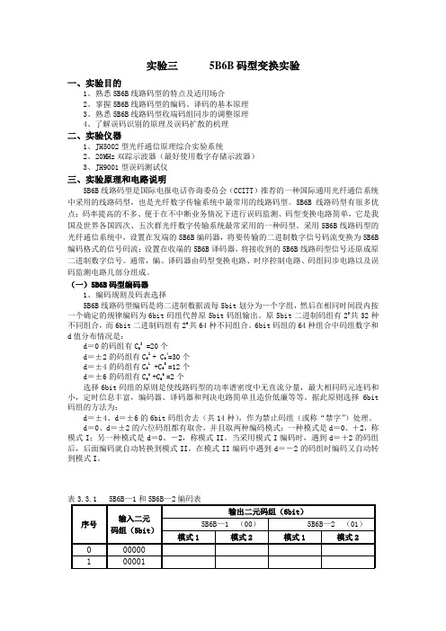
(一)5B6B码型编码器1、编码规则及码表选择5B6B线路码型编码是将二进制数据流每5bit划分为—个字组,然后在相同时间段内按一个确定的规律编码为6bit码组代替原5bit码组输出。
原5bit二进制码组有25共32种不同组合,而6bit二进制码组有26共64种不同组合。
6bit码组的64种组合中码组数字和d值分布情况是:d=0的码组有C63 =20个d=±2的码组有C62 + C64=30个d=±4的码组有C61 +C65 =12个d=±6的码组有C60 +C66 =2个选择6bit码组的原则是使线路码型的功率谱密度中无直流分量,最大相同码元连码和小,定时信息丰富,编码器、译码器和判决电路简单且造价低廉等等。
据此原则选择6bit 码组的方法为:d=±4、d=±6的6bit码组舍去(共14种),作为禁止码组(或称“禁字”)处理。
Infineon TLE4966-2K高精度双输出电磁感应切换器数据手册(版本1.0)说明书

TLE4966-2KHigh Precision Hall Switch with two OutputsDatasheetRev.1.0, 2010-06-28Edition 2010-06-28Published byInfineon Technologies AG81726 Munich, Germany© 2010Infineon Technologies AGAll Rights Reserved.Legal DisclaimerThe information given in this document shall in no event be regarded as a guarantee of conditions or characteristics. With respect to any examples or hints given herein, any typical values stated herein and/or any information regarding the application of the device, Infineon Technologies hereby disclaims any and all warranties and liabilities of any kind, including without limitation, warranties of non-infringement of intellectual property rights of any third party.InformationFor further information on technology, delivery terms and conditions and prices, please contact the nearest Infineon Technologies Office ().WarningsDue to technical requirements, components may contain dangerous substances. For information on the types in question, please contact the nearest Infineon Technologies Office.Infineon Technologies components may be used in life-support devices or systems only with the express written approval of Infineon Technologies, if a failure of such components can reasonably be expected to cause the failure of that life-support device or system or to affect the safety or effectiveness of that device or system. Life support devices or systems are intended to be implanted in the human body or to support and/or maintain and sustain and/or protect human life. If they fail, it is reasonable to assume that the health of the user or other persons may be endangered.TLE4966-2KRevision History: 2010-06-28, Rev.1.0Previous Revision:Page Subjects (major changes since last revision)Trademarks of Infineon Technologies AGABM™, BlueMoon™, CONVERGATE™, COSIC™, C166™, FALC™, GEMINAX™, GOLDMOS™, ISAC™, OMNITUNE™, OMNIVIA™, PROSOC™, SEROCCO™, SICOFI™, SIEGET™, SMARTi™, SMINT™, SOCRATES™, VINAX™, VINETIC™, VOIPRO™, X-GOLD™, XMM™, X-PMU™, XWAY™Other TrademarksMicrosoft®, Visio®, Windows®, Windows Vista®, Visual Studio®, Win32® of Microsoft Corporation. Linux® of Linus Torvalds. FrameMaker®, Adobe® Reader™, Adobe Audition® of Adobe Systems Incorporated. APOXI®, COMNEON™ of Comneon GmbH & Co. OHG. PrimeCell®, RealView®, ARM®, ARM® Developer Suite™ (ADS), Multi-ICE™, ARM1176JZ-S™, CoreSight™, Embedded Trace Macrocell™ (ETM), Thumb®, ETM9™, AMBA™, ARM7™, ARM9™, ARM7TDMI-S™, ARM926EJ-S™ of ARM Limited. OakDSPCore®, TeakLite® DSP Core, OCEM® of ParthusCeva Inc. IndoorGPS™, GL-20000™, GL-LN-22™ of Global Locate. mipi™ of MIPI Alliance. CAT-iq™ of DECT Forum. MIPS™, MIPS II™, 24KEc™, MIPS32®, 24KEc™ of MIPS Technologies, Inc. Texas Instruments®, PowerPAD™, C62x™, C55x™, VLYNQ™, Telogy Software™, TMS320C62x™, Code Composer Studio™, SSI™ of Texas Instruments Incorporated. Bluetooth® of Bluetooth SIG, Inc. IrDA® of the Infrared Data Association. Java™, SunOS™, Solaris™ of Sun Microsystems, Inc. Philips®, I2C-Bus® of Koninklijke Philips Electronics N.V. Epson® of Seiko Epson Corporation. Seiko® of Kabushiki Kaisha Hattori Seiko Corporation. Panasonic® of Matsushita Electric Industrial Co., Ltd. Murata® of Murata Manufacturing Company. Taiyo Yuden™of Taiyo Yuden Co., Ltd. TDK® of TDK Electronics Company, Ltd. Motorola® of Motorola, Inc. National Semiconductor®, MICROWIRE™ of National Semiconductor Corporation. IEEE® of The Institute of Electrical and Electronics Engineers, Inc. Samsung®, OneNAND®, UtRAM® of Samsung Corporation. Toshiba® of Toshiba Corporation. Dallas Semiconductor®, 1-Wire® of Dallas Semiconductor Corp. ISO® of the International Organization for Standardization. IEC™ of the International Engineering Consortium. EMV™ of EMVCo, LLC. Zetex® of Zetex Semiconductors. Microtec® of Microtec Research, Inc. Verilog® of Cadence Design Systems, Inc. ANSI® of the American National Standards Institute, Inc. WindRiver® and VxWorks® of Wind River Systems, Inc. Nucleus™ of Mentor Graphics Corporation. OmniVision® of OmniVision Technologies, Inc. Sharp® of Sharp Corporation. Symbian OS® of Symbian Software Ltd. Openwave® of Openwave Systems, Inc. Maxim® of Maxim Integrated Products, Inc. Spansion® of Spansion LLC. Micron®, CellularRAM® of Micron Technology, Inc. RFMD® of RF Micro Devices, Inc. EPCOS® of EPCOS AG. UNIX® of The Open Group. Tektronix® of Tektronix, Inc. Intel® of Intel Corporation. Qimonda® of Qimonda AG. 1GOneNAND® of Samsung Corporation. HyperTerminal® of Hilgraeve, Inc. MATLAB® of The MathWorks, Inc. Red Hat® of Red Hat, Inc. Palladium® of Cadence Design Systems, Inc. SIRIUS Satellite Radio® of SIRIUS Satellite Radio Inc. TOKO® of TOKO Inc.The information in this document is subject to change without notice.Last Trademarks Update 2008-11-17Trademarks of Infineon Technologies AG . . . . . . . . . . . . . . . . . . . . . . 31Overview . . . . . . . . . . . . . . . . . . . . . . . . . . . . . . . . . . . . . . . . . . . . . . . . . . . 5 1.1Features . . . . . . . . . . . . . . . . . . . . . . . . . . . . . . . . . . . . . . . . . . . . . . . . . . . . 5 1.2Functional Description . . . . . . . . . . . . . . . . . . . . . . . . . . . . . . . . . . . . . . . . . 5 1.3Pin Configuration (top view) . . . . . . . . . . . . . . . . . . . . . . . . . . . . . . . . . . . . . 62General . . . . . . . . . . . . . . . . . . . . . . . . . . . . . . . . . . . . . . . . . . . . . . . . . . . . 7 2.1Block Diagram . . . . . . . . . . . . . . . . . . . . . . . . . . . . . . . . . . . . . . . . . . . . . . . 7 2.2Circuit Description . . . . . . . . . . . . . . . . . . . . . . . . . . . . . . . . . . . . . . . . . . . . 7 2.3Application Circuit . . . . . . . . . . . . . . . . . . . . . . . . . . . . . . . . . . . . . . . . . . . . 8 3Maximum Ratings . . . . . . . . . . . . . . . . . . . . . . . . . . . . . . . . . . . . . . . . . . . 84Operating Range . . . . . . . . . . . . . . . . . . . . . . . . . . . . . . . . . . . . . . . . . . . . 95Electrical and Magnetic Parameters . . . . . . . . . . . . . . . . . . . . . . . . . . . 10 Field Direction Definition . . . . . . . . . . . . . . . . . . . . . . . . . . . . . . . . . . 11 6Timing Diagrams for the Speed Outputs . . . . . . . . . . . . . . . . . . . . . . . . 11 7Package Information . . . . . . . . . . . . . . . . . . . . . . . . . . . . . . . . . . . . . . . . 12 7.1Package Marking . . . . . . . . . . . . . . . . . . . . . . . . . . . . . . . . . . . . . . . . . . . . 12 7.2Distance between Chip and Package Surface . . . . . . . . . . . . . . . . . . . . . . 12 7.3Package Outlines . . . . . . . . . . . . . . . . . . . . . . . . . . . . . . . . . . . . . . . . . . . . 12PCB Footprint for PG-TSOP6-6-5 . . . . . . . . . . . . . . . . . . . . . . . . . . . 13Product Name Product Type Ordering Code Package TLE4966-2K Double Hall SwitchSP000788888PG-TSOP6-6-5High Precision Hall Switch with two OutputsTLE4966-2K1Overview1.1Features• 2.7V to 24V supply voltage operation•Operation from unregulated power supply •High sensitivity and high stability of the magnetic switching points•High resistance to mechanical stress by Active Error Compensation •Reverse battery protection (-18V)•Superior temperature stability •Peak temperatures up to 195°C •Low jitter (typ. 1μs)•Digital output signals•Excellent matching of the 2 Hall probes •Hall plate distance 1.45mm•Two independent speed outputs •SMD package PG-TSOP6-6-51.2Functional DescriptionThe TLE4966-2K is an integrated circuit dual Hall-effect sensor designed specifically for highly accurate applications. Precise magnetic switching points and high temperature stability are achieved by active compensation circuits and chopper techniques on chip. The sensor provides two independent speed outputs at Q1 and Q2 with the status (high or low) corresponding to the magnetic field value at the respective Hall element H1 and H2. Both Hall elements have the identical thresholds for B OP and B RP (B OP1 = B OP2 and B RP1 = B RP2). For positive magnetic fields (south pole) exceeding the threshold B OP1 and/or B OP2 the corresponding output Q1 and/or Q2 is low, whereas for negative magnetic fields (north pole) lower than B RP the output switches to high. Due to the spatial distance of the two Hall elements on the chip (d = 1.45mm) the two output signals will show a phase difference in case the sensor is used with a rotating magnetized pole wheel.Overview 1.3Pin Configuration (top view)Table 1Pin Definitions and FunctionsPin No.Symbol Function1Q2Speed 22GND Recommended connection to GND3Q1Speed 14V DD Supply voltage5GND Recommended connection to GND6GND GroundGeneral 2General2.1Block Diagram2.2Circuit DescriptionThe chopped Dual Hall Switch comprises two Hall probes, bias generator, compensation circuits, oscillator, and output transistors.The bias generator provides currents for the Hall probes and the active circuits. Compensation circuits stabilize the temperature behavior and reduce influence of technology variations.The Active Error Compensation rejects offsets in signal stages and the influence of mechanical stress to the Hall probes caused by molding and soldering processes and other thermal stresses in the package. This chopper technique together with the threshold generator and the comparator ensures high accurate magnetic switching thresholds.Maximum Ratings2.3Application CircuitIt is recommended to use a series resistor R S with 200Ω and a capacitor of C S = 4.7nF for protection againstFigure 3Application Circuit3Maximum RatingsNote:Stresses above those listed here may cause permanent damage to the device. Exposure to absolutemaximum rating conditions for extended periods may affect device reliability. Maximum ratings are absolute ratings; exceeding only one of these values may cause irreversible damage to the integrated circuit.Table 2Absolute Maximum Ratings T j = -40°C to 150°CParameterSymbolLimit Values UnitConditionsmin.max.Supply voltageV DD V s V s -18 -18 -1818 24 26Vfor 1 h, R S ≥ 200 Ω for 5 min, R S ≥ 200 ΩSupply current through protection device I DD-5050mAOutput voltage V Q -0.7 -0.718 26V************Ω pull upContinuous output current I Q -5050mA Junction temperatureT j– – – –155 165 175 195°Cfor 2000 h (not additive) for 1000 h (not additive) for 168 h (not additive) for 3 x 1 h (additive)Storage temperature T S -40150°C Magnetic flux densityB–unlimitedmTTable 3ESD Protection 1)1)Human Body Model (HBM) tests according to: EOS/ESD Association Standard S5.1-1993 and Mil. Std. 883D method3015.7Parameter SymbolLimit Values UnitNotesmin.max.ESD voltageV ESD–±4kVHBM , R = 1.5 k Ω, C = 100 pF T A = 25°COperating Range4Operating RangeThe following operating conditions must not be exceeded in order to ensure correct operation of the TLE4966-2K. All parameters specified in the following sections refer to theses operating conditions unless otherwise mentioned.Table 4Operating RangeParameter SymbolLimit Values UnitConditionsmin.typ.max.Supply voltageV DD V S V S 2.7 – –– – –18 24 26V1 h with R S ≥ 200 Ω for 5 min R S ≥ 200 ΩOutput voltage V Q -0.7–18V Junction temperature T j -40 –– –150 175°Cfor 168 hOutput currentI Q–10mAElectrical and Magnetic Parameters5Electrical and Magnetic ParametersProduct characteristics involve the spread of values guaranteed within the specified voltage and temperature range. Typical characteristics are the median of the production.Table 5Electrical Characteristics 1)1)over operating range, unless otherwise specified. Typical values correspond to V DD = 12 V and T A = 25°CParameter SymbolLimit Values UnitConditionsmin.typ.max.Supply currentI DD4 5.27mA V DD = 2.7 V ... 18 V Reverse current I SR 00.21mA V DD = -18 V Output saturation voltage V QSAT –0.30.6V I Q = 10 mA Output leakage current I QLEAK –0.0510μA for V Q = 18 VOutput fall time t f –0.21μs R L = 1.2 k Ω; C L < 50 pFsee: Figure 4 on Page 11Output rise time t r –0.21μs Chopper frequency f OSC –320–kHz Switching frequency f SW 0–15 2)2)To operate the sensor at the max. switching frequency, the magnetic signal amplitude must be 1.4 times higher than forstatic fields. This is due to the -3 dB corner frequency of the low pass filter in the signal path.kHz Delay time 3)3)Systematic delay between magnetic threshold reached and output switching t d –13–μs Count Signal Delay t dc 502001000nsOutput jitter 4)4)Jitter is the unpredictable deviation of the output switching delay t QJ –1–μs RMS Typ. value for square wave signal 1 kHz Repeatability of magnetic thresholds5)5)B REP is equivalent to the noise constantB REP–40–μT RMS Typ. value for ΔB /Δt > 12 mT/ms Power-on time 6)6)Time from applying V DD ≥ 2.7 V to the sensor until the output state is valid t PON –13–μs V DD ≥ 2.7 VDistance of hall plates d HALL – 1.45–mm Thermal resistance 7)7)Thermal resistance from junction to ambientCalculation of the ambient temperature (PG-TSOP6-6-5 example)e.g. for V DD = 12.0 V, I DDtyp = 5.5 mA, V QSATtyp = 0.3 V and 2 x I Q = 10 mA : Power Dissipation: P DIS = 72.0 mW.In T A = T j – (R thJA × P DIS ) = 175°C – (100 K / W × 0.072 W) Resulting max. ambient temperature: T A = 167.8°CR thJA–100–K/WPG-TSOP6-6-5Timing Diagrams for the Speed OutputsNote:Typical characteristics specify mean values expected over the production spread.Field Direction DefinitionPositive magnetic fields related with south pole of the magnet to the branded side of package.6Timing Diagrams for the Speed OutputsTable 6Magnetic Characteristics 1).1)over operating range, unless otherwise specified. Typical values correspond to V DD = 12 VParameterSymbolT j[°C]Limit Values Unit Conditionsmin.typ.max.Operate pointB OP1, B OP2-40 25 150 5.2 5.0 4.77.7 7.5 7.110.3 10.0 9.5mTB OP1 for Hall element 1 B OP2 for Hall element 2Release pointB RP1, B RP2-40 25 150-10.3 -10.0 -9.5-7.7 -7.5 -7.1-5.2 -5.0 -4.7mTB RP1 for Hall element 1 B RP2 for Hall element 2HysteresisB HYS1, B HYS2-40 25 150– 10.0 –– 15.0 –– 20.0 –mTB HYS1 = B OP1 - B RP1 B HYS2 = B OP2 - B RP2Magnetic matchingB MATCH-40 25 150– -2.0 –– 0 –– 2.0 –mTValid forB OP1 - B OP2 and B RP1 - B RP2Magnetic offsetB OFF1, B OFF2-40 25 150– -2.0 –– 0 –– 2.0 –mTB OFF1 = (B OP1 + B RP1)/2 B OFF2 = (B OP2 + B RP2)/2Temperaturecompensation of magnetic thresholdsTC ––-350–ppm/°C7Package Information7.1Package MarkingFigure 5Marking PG-TSOP6-6-57.2Distance between Chip and Package SurfaceFigure 6Distance Chip to Upper Side of IC7.3Package OutlinesPCB Footprint for PG-TSOP6-6-5Figure 8Footprint PG-TSOP6-6-5You can find all of our packages, sorts of packing and others in ourInfineon Internet Page “Products”: /products.Dimensions in mmw w w.i n f i n e o n.c o mMouser ElectronicsAuthorized DistributorClick to View Pricing, Inventory, Delivery & Lifecycle Information:I nfineon:TLE4966-2K。
全国计算机等级考试一级B必过练习之Word操作题练习

2011年全国计算机等级考试一级B必过练习之Word操作题练习2011年全国计算机等级考试一级B必过练习之Word操作题练习(一)考题类型根据历次考试的情况,字表处理部分的考题一般由2到3个题目组成,其操作类型有以下几种:(1)多窗口操作;(2)文字输入(包括汉字、英文、特殊符号及全角/半角的切换);(3)文档的分段、合并及复制,文档的替换;(4)设置字体(各种汉字及英文字体)、字型、字号及字符的修饰(设置颜色、下划线、上标、下标及各种字体效果等);(5)段落排版中的缩进(左、右缩进及特殊格式)、间距(段前、段后行间距)、对齐方式(左、右、居中、两端及分散方式);(6)分栏设置(栏数目、栏间距、栏宽度、分隔线的设置);(7)表格制作(插入表格,增加表格的行列,改变行列宽度,单元格的合并及拆分,表格内字符的重新设置)、表格排序、表格内字符的删除及表格删除;(8)页边距设置;(9)文档的保存(指定文件及文件名)。
(二)考试要点(1)单击“字表处理”按钮后,屏幕窗口显示Word部分考题内容,考试时不能直接在题目窗口编辑排版,应按考题要求启动Word,打开指定的文件,在Word 编辑窗口编辑该文件;(2)考生应看清题目后,严格按题目顺序逐项进行操作,争取一次成功。
如果操作有误可撤销上一步操作。
切记:综合考虑后按自己的理解进行;(3)编辑排版操作后,根据题目要求,确定无误后,再按指定文件夹及指定文件名保存文件。
(三)编辑排版操作说明(1)启动Word文档显示Word题目后按Alt+F5键将题板缩小,然后启动Word字表处理软件,并调整两个窗口的位置,再按题目要求输入文档内容。
(2)文档复制拖动鼠标选定要复制的内容→单击常用工具条上的“复制”命令按钮→将光标移到复制的目的位置→单击常用工具条上的“粘贴”按钮。
(3)替换文档内容打开“编辑”菜单→选择“替换”选项→打开“替换”对话框→在对话框中输入查找对象和替换对象→单击“替换”按钮(逐个替换)或“全部替换”按钮(全部替换)。
- 1、下载文档前请自行甄别文档内容的完整性,平台不提供额外的编辑、内容补充、找答案等附加服务。
- 2、"仅部分预览"的文档,不可在线预览部分如存在完整性等问题,可反馈申请退款(可完整预览的文档不适用该条件!)。
- 3、如文档侵犯您的权益,请联系客服反馈,我们会尽快为您处理(人工客服工作时间:9:00-18:30)。
结合探索性数据分析技术/统计图 不用盲目选择ladder给出的统计检验结果
进一步阅读 • Fox J, 1997, Applied regression analysis, linear models, and related methods, Sage.
– Chapter 3 on examining data – Chapter 4 on transforming data – Note the recommended reading at the end of each chapter
log spread = 0.37 + 0.80 * log median pow er = 1 - b =0.2 0
80
60
s
1.2
40
1.1
20
1.0
0
CAN
OTH
UK
US
0.8
0.9 m
1.0
1.1
1.2
0
1
2
3
4
CAN
OTH
UK
US
相关的Stata命令 • ladder • gladder • qladder
12 12 2.5 l$y -2 -1 0 x2 1 2 3 0.5 2 3 x 4 5 0 1.0 4 2 2 1.5 6 y2 y 4 6 2.0 8 8
10
10
-1.5
-1.0
-0.5
0.0 l$x
0.5
1.0
1.5
参考规则
y ,y
2 3
logx, x
x ,x
2
3
logy, y
参考规则的应用
数据变换
黄荣贵
为什么数据变换
• 通过数据变换使数据的分布接近统计模型的界定 • 数据变换也有助于研究者更好地查看数据关系 • 变换的目的包括
– – – – 分布对称性 两变量的关系线性 不同组群等方差 ……
如何检验变换后的新变量是否令人满意?
幂变换
•
– 除p确保变换后的全部x具有相同的方向 – 实际应用中,P往往取值为-2到3
2.0
2.5
3.0
x, ratior=1.003
x-1990, ratio=6 0.5 0.0 1991
1992
1993 x
1994
1995
1996
变换偏度
• 为什么要使数据对称?
– 非对称数据比较难以解读 – 对与偏度一致的数据而言,表面异常数据可能不是异常;方向不 一致的数据,可能的异常案例被大量数据所掩盖 – 如果统计方法依赖于均值,则偏度数据对结果有很大的影响
• Log10x=0.4343*Ln(x)
幂变换的局限与应用
• 局限
– 部分变换对0和负数无定义 – 部分变换不是单调递增函数(比如2次方) – 当最大值和最小值的比比较小(小于5),变换效果不明显 – X -> (X+S)(p)
Transformed values 3.5
• 处理方式
1.0
1.5
Density
注意分布两端可 能的异常值分布
0.00000 0
5000
10000
15000
20000
25000
30000
Transformed Variable
1.5 Density 0.0 100 0.5 1.0
1000
10000
31622
线性变换
• •
8
为什么变换——线性关系容易解读,线性回归模型广泛应用、相关统 计理论比较成熟、系统,数据稀薄时非线性关系难以准确估计 幂变换可以使变量关系线性化,比如
y vs x y vs x y vs x
2
6
2.5
yn
y
2.0
4
y 1.5 0.5 1.0 1.0 1.5 2.0 2.5 x 3.0 3.5 4.0 0 0 2 4
0
2
1.0
1.5
2.0
2.5 x
3.0
3.5
4.0
6
8
5 xn
10
15
线性变换
• 只有简单单调曲线关系可以通过幂变换线性化
– 即第一种关系 – 曲线每一点的一阶导数都为正/负,并且逐渐增加/减少
1.00 -0.25
0.75
-0.50
0.50
x^-1/-1
-0.75 0.25 -1.00 2 4 6 2 4 6
x^-1
x
x
– 所有变换后的曲线经过1/0点(并且斜率为1)
6
注意不同变换对数值 大小(差异)的影响
(x^-1 - 1)/-1
-4 0
-2
0
2
4
1
2
3 x
4
5
6
– X(0)定义为以自然对数Ln(x)
80
60
Prestige$prestige
40
Prestige$prestige 0 5000 10000 15000 20000 25000
20
20
40
60
80
10
15
20 Prestige$income^(1/3)
25
30
Prestige$income
UN$infant.mortality 0 0 10000 20000 30000 40000 log(UN$infant.mortality) 1 2 3 4 5 4 5 6 7 8 9 10 log(UN$gdp) UN$gdp 50 100 150
应用(2)
幂变换与组间变异
• 参考规则(Stabilizing the variance)
– If Log spread = a + b * log(level such as median) – Then power p = 1 – b
interlocks Choice of power
100
1.3
• 幂变换可以消减偏度的影响
– 参考性指标
≅ 1,检查几个可能的变换,பைடு நூலகம்要
机械选择最接近1的变换方法 – 正偏 -> 降幂(比如取对数) – 负偏 -> 升幂(比如2次方、3次方)
课后练习
• 如果同样效果的变换,优先选择容易解读的方式
正偏态数据对数转换
Original Variable
0.00008