北大暑期课程《回归分析》(Linear Regression Analysis)讲义PKU5

合集下载

北大暑期课程回归分析(I)

《回归分析》教学大纲

回归分析RegressionAna1ysis一、课程基本信息课程编号：111093适用专业：统计学专业课程性质：专业必修开课单位：数学与数据科学学院学时：48（理论学时40；实验学时8）学分：3考核方式：考试（平时成绩占30%+考试成绩70%）中文简介：回归分析是应用统计学中一个重要的分支，在自然科学、管理科学和社会经济等领域应用十分广泛。

《回归分析》课程是统计学专业的学科专业必修课是学生掌握统计学的基本思想、理论和方法的主要课程，是培养学生熟练应用计算机软件处理统计数据的能力的基础课程。

通过本课程的学习，使学生掌握应用统计的一些基本理论与方法，初步掌握利用回归分析解决实际问题的能力。

二、教学目的与要求本课程的主要目的是学生在学习后，能够系统掌握回归分析的理论与方法，并在此基础上，掌握回归分析应用的艺术技巧，并利用其分析认识实际问题。

本课程注重回归分析的基本理论与方法，同时通过案例教学与实际应用来剖析回归分析的理论与方法所蕴含的统计思想及其应用艺术。

教学中在回归分析理论与方法的基础上结合社会、经济、自然学科学领域的研究实例，把回归分析方法与实际应用结合起来，注重定性分析与定量分析的紧密结合，强调每种方法的优缺点和实际运用中应注意的问题,研究与实践中应用回归分析的经验和体会融入其中，使学生充分体会到回归分析的应用艺术，并提高解决问题的能力。

通过本课程的学习，在理论教学过程中，可以结合国内外回归分析相关学者的研究经历和成果，传播科学研究所需要的实事求是、脚踏实地的精神，培养学生的科学素养。

在实践教学中，利用案例分析、软件仿真等方式培养学生的实践能力和创新思维，激发学生主动研究新问题和设计新方法的兴趣，让学生在实践中深刻体会科学研究的乐趣，也可以鼓励有突出能力的学生通过创新创业或成果转化为社会发展贡献年轻的力量。

三、教学方法与手段1.教学方法：课堂讲授中要重点对基本概念、基本方法和解题思路的讲解；采用启发式教学，培养学生思考问题、分析问题和解决问题的能力；引导和鼓励学生通过实践和自学获取知识，培养学生的自学能力和创新能力。

北大暑期课程《回归分析》(Linear-Regression-Analysis)讲义pku4教学教材

Class 4: Inference in multiple regression.I. The Logic of Statistical InferenceThe logic of statistical inference is simple: we would like to make inferences about a population from what we observe from the sample that has been drawn randomly from the population.The samples' characteristics are called "point estimates."It is almost certain that the sample's characteristics are somewhat different from the population's characteristics. But because the sample was drawn randomly from the population, the sample's characteristics cannot be "very different" from thepopulation's characteristics. What do I mean by "very different"? To answer this question, we need a distance measure (or dispersion measure), called the standard deviation of the statistic.To summarize, statistical inferences consist of two steps:(1) Point estimates (sample statistics) (2) Standard deviations of the point estimates (dispersion of sample statisticsin a hypothetical sampling distribution).II. Review: For a sample of fixed size y n i ,,1 =is the dependent variable;11,,1-=p x x X contains independent variables.We can write the model in the following way: ,εβ+=X yUnder certain assumptions, the LS estimator 1()b X X X y -''=As certain desirable properties:A1 => unbiasedness and consistency A1 + A2 => BLUE, with 12()()V b X X σ-'= A1 + A2 + A3 =>BUE 12()()V b X X σ-'= (even for small samples)III. The Central Limit Theorem Statement: The mean of iid random variables (with mean of μ, and variance of 2σ) approaches a normal distribution as the number of random variables increases. ∞→→n n N X n as ),/,(2σμThe property belongs to the statistic -- sample mean in the sampling distribution of all sample means, even though the random variables themselves are not normally distributed. You can never check this normality because you can only have one sample statistic.In regression analysis, we do not assume that ε is normally distributed if we have a large sample, because all estimated parameters approach to normal distributions. Why: all LS estimates are linear function of ε (proved last time). Recall a theorem: a linear transformation of a variable distributed as normal is also distributed as normal.IV. Inferences about Regression CoefficientsA. Presentation of Regression ResultsCommon practice: give a star beside the parameter estimate for significance level of 0.05, two stars for 0.01, and three stars for 0.001. For example: Dependent Variable: EarningsIndependent Variable:Father's education 0.900*Mother's education 0.501***Shoe size -2.16What is the problem with this practice?First, we want to have a quantitative evaluation of the significance level. We should not blindly rely on statistical tests. For example,Father's education 0.900* (0.450)Mother's education 0.501*** (0.001)Shoe size -2.16 (1.10)In this case, is father's education much more significant than shoe size? Not really. They are very similar. By contrast, mother's is far more significant than the other two.A second practice is to report the t or z values:Coeffi. t.Father's education 0.900 2.0Mother's education 0.501 500.Shoe size -2.16 -1.96This solution is much better. However, very often, our hypothesis is not about deviation from zero, but from other hypothetical values. For example, we are interested in the hypothesis whether a one-year increase in father's education will increase son's education by one year. The hypothesis here is 1 instead of 0.The preferred way of presentation is:Coeff. (S.E.) Father's education0.900 (0.450) Mother's education0.501 (0.001) Shoe size -2.16 (1.10)B. Difference between Statistical Significance and the Size of an EffectStatistical significance always refers to a stated hypothesis. You will see a lot of misuses in the literature, sometimes by well-known sociologists. They would saythat this variable is highly significant. That one is not significant. This is not correct. I am not responsible for their mistakes, but I want to warn you not to commit the same mistakes again. In our example, you could say Mother's education is highly significant from zero. But it is not significant from 0.5. Had your hypothesis been that the parameter for Mother's education is 0.5, the result would be consistent with the hypothesis. That is, statistical significance should always be made with reference to a hypothesis. Follow2/)(022b SE b z β-= Another common mistake is to equate statistical significance with the size of an effect. A variable can be statistically significant from zero. But the estimated coefficient is small. The contribution of father's education to the dependent variable is larger than that of mother's education even though mother's education is more statistically significant from zero than father's education.Important: you should look at both coefficients and their standard errors.C. Confidence Intervals for Single Parameters)(96.1j j j b SE b ±=βD. Hypothesis Testing for Single ParametersCompare )(/)(0j j j b SE b z β-=, if z is outside the range of -1.96 and 1.96, the hypothesis is rejected. Otherwise, we fail to reject the hypothesis.V. Inferences about Linear Combinations of Two ParametersExample 1: 21ββ=(equality hypothesis), ==> 021=-ββExample 2: 2110ββ=(proportionality hypothesis), ==>01021=-ββExample 3: 221+=ββ (surplus hypothesis), ==> 221=-ββIn general form, we may have )(2211γββ=+c cHypothesis testing:c c c =+2211ββ Confidence interval:2211ββc c + lies between (low limit, upper limit)Procedure:A. Point estimate:Compute 2211b c b c +B. Degree of Imprecision),(2)()()(21212221212211b b Cov c c b V c b V c b c b c V ++=+ and then take square root of )(2211b c b c V +.We would need to obtain the variance-covariance matrix of the parameter vector in order to carry out the calculation.)( and )(21b V b V are on the diagonal,),(21b b Cov is off-diagonal.Let us look at the first half the example. Compute the confidence interval for the hypothesis that β1=β2.Step 1. b 1 - b 2 = 5732.0- 3146.0 = 0.2586.Step 2: V(b 1 - b 2) = 0642.0+ 0310.0-2* (0227.0-) = 0.1406.SD(b 1 - b 2) = 0.14061/2 = 0.3750.Step 3:Computet 2 = (0.2586 -0)/ 0.3750 = 0.6897, insignificant (unsurprising result).Note DF = 5-3 = 2.I use two parameters as an example.Examples of Hypothesis Testing:Example 1: 21ββ=(equality hypothesis), ==>021=-ββExample 2: 2110ββ=(proportionality hypothesis), ==>01021=-ββExample 3: 221+=ββ(surplus hypothesis), ==>221=-ββIn general form,We may have ()γββ=+ c c 2211Hypothesis testing: c c c 2211=+ββConfidence interval: 2211c c ββ+ lies between (low limit, upper limit)Procedure:A. Find point estimate:Compute 1c 1b +2c 2bB. Find degree of Imprecision ()()()()21212221212211b ,b Cov c c 2b V c b V c b c b c V ++=+ and then take square root of ()2211b c b c V +.We would need to obtain the variance-covariance matrix of the parameter vector in order to carry out the calculation.V(1b ) and V(2b ) are on the diagonal,Cov(1b ,2b ) is off-diagonal.Numerical Example: Multiple regressions For the following small data set (n = 5), use matrix operations to solve the following problems. You should make use of the information below as much as possible. Let[][][][]65420',40201',42301',12121====X x x y x xIt is known that⎥⎥⎥⎦⎤⎢⎢⎢⎣⎡=X X 813271775' ⎥⎥⎥⎦⎤⎢⎢⎢⎣⎡=X 4610'y⎥⎥⎥⎦⎤⎢⎢⎢⎣⎡------=X X -0582.0426.1381.0426.1205.0239.1381.0239.7030.)'(11. Write out X and y in full.1112212231324142515211101110201,12431105211464x x x x x x y x x x x ⎡⎤⎡⎤⎡⎤⎢⎥⎢⎥⎢⎥⎢⎥⎢⎥⎢⎥⎢⎥⎢⎥⎢⎥X ===⎢⎥⎢⎥⎢⎥⎢⎥⎢⎥⎢⎥⎢⎥⎢⎥⎢⎥⎣⎦⎣⎦⎣⎦ 2. Write X X 'and y X 'in full.57171072132,2317328146X X X y ⎡⎤⎡⎤⎢⎥⎢⎥''==⎢⎥⎢⎥⎢⎥⎢⎥⎣⎦⎣⎦3. Estimate b with the help of a calculator (b is the least squares estimator of β, the regression coefficients of X ).10.703 -0.024 -0.138 100.128 (')'-0.024 0.120 -0.043 230.573 -0.138 -0.043 0.058 460.315 b X X X y -⎡⎤⎡⎤⎡⎤⎢⎥⎢⎥⎢⎥===⎢⎥⎢⎥⎢⎥⎢⎥⎢⎥⎢⎥⎣⎦⎣⎦⎣⎦4. Find the predicted values for y .0.701 1100.128 0.757 1020.573 2.533 1240.315 1.701 105 4.308 146y X b ⎡⎤⎡⎤⎢⎥⎢⎥⎡⎤⎢⎥⎢⎥⎢⎥⎢⎥⎢⎥===⎢⎥⎢⎥⎢⎥⎢⎥⎣⎦⎢⎥⎢⎥⎢⎥⎢⎥⎣⎦⎣⎦5. Calculate SST, SSR, and SSE. (Hint: to obtain SSR, you may use the results from 4.222222222222222222222222222()(12)(02)(32)(22)(42)10103245210()(0.7012)(0.7572)(2.5332)(1.7012)(4.3082)8.9350.7010.757 2.533 1.701 4.308i i i i SST Y Y Y nY SSR Y Y Y nY =-=-+-+-+-+-==-=++++-⨯==-=-+-+-+-+-==-=++++=∑∑∑∑8.935108.935 1.065SSE SST SSR =-=-= 6. Calculate the variance-covariance matrix of b . 1110.703 -0.024 -0.138 0.375 -0.013 -0.074 1.065()(')'()(')(')-0.024 0.120 -0.043 -0.013 0.064 -0.023 53-0.138 -0.043 0.058 -0.074 -0.023 0.031 V b X X X V e X X X X X MSE ---⎡⎤⎡⎤⎢⎥⎢⎥===*=⎢⎥⎢⎥-⎢⎥⎢⎥⎣⎦⎣⎦。

北大暑期课程《回归分析》(Linear-Regression-Analysis)讲义1汇编

Class 1: Expectations, variances, and basics of estimationBasics of matrix (1)I. Organizational Matters(1)Course requirements:1)Exercises: There will be seven (7) exercises, the last of which is optional. Eachexercise will be graded on a scale of 0-10. In addition to the graded exercise, ananswer handout will be given to you in lab sections.2)Examination: There will be one in-class, open-book examination.(2)Computer software: StataII. Teaching Strategies(1) Emphasis on conceptual understanding.Yes, we will deal with mathematical formulas, actually a lot of mathematical formulas. But, I do not want you to memorize them. What I hope you will do, is to understand the logic behind the mathematical formulas.(2) Emphasis on hands-on research experience.Yes, we will use computers for most of our work. But I do not want you to become a computer programmer. Many people think they know statistics once they know how to run a statistical package. This is wrong. Doing statistics is more than running computer programs. What I will emphasize is to use computer programs to your advantage in research settings. Computer programs are like automobiles. The best automobile is useless unless someone drives it. You will be the driver of statistical computer programs.(3) Emphasis on student-instructor communication.I happen to believe in students' judgment about their own education. Even though I will be ultimately responsible if the class should not go well, I hope that you will feel part of the class and contribute to the quality of the course. If you have questions, do not hesitate to ask in class. If you have suggestions, please come forward with them. The class is as much yours as mine.Now let us get to the real business.III(1). Expectation and VarianceRandom Variable: A random variable is a variable whose numerical value is determined by the outcome of a random trial.Two properties: random and variable.A random variable assigns numeric values to uncertain outcomes. In a common language, "give a number". For example, income can be a random variable. There are many ways to do it. You can use the actual dollar amounts.In this case, you have a continuous random variable. Or you can use levels of income, such as high, median, and low. In this case, you have an ordinal random variable [1=high,2=median, 3=low]. Or if you are interested in the issue of poverty, you can have a dichotomous variable: 1=in poverty, 0=not in poverty.In sum, the mapping of numeric values to outcomes of events in this way is the essence of a random variable.Probability Distribution: The probability distribution for a discrete random variable X associates with each of the distinct outcomes x i(i = 1, 2,..., k) a probability P(X = x i).Cumulative Probability Distribution: The cumulative probability distribution for a discrete random variable X provides the cumulative probabilities P(X ≤ x) for all values x.Expected Value of Random Variable: The expected value of a discrete random variable X is denoted by E{X} and defined:E{X}=(x i)where: P(x i) denotes P(X = x i). The notation E{ } (read “expectation of”) is called the expectation operator.In common language, expectation is the mean. But the difference is that expectation is a concept for the entire population that you never observe. It is the result of the infinite number of repetitions. For example, if you toss a coin, the proportion of tails should be .5 in the limit. Or the expectation is .5. Most of the times you do not get the exact .5, but a number close to it.Conditional ExpectationIt is the mean of a variable conditional on the value of another random variable.Note the notation: E(Y|X).In 1996, per-capita average wages in three Chinese cities were (in RMB):Shanghai: 3,778Wuhan: 1,709Xi’an: 1,155Variance of Random Variable: The variance of a discrete random variable X is denoted by V{X} and defined:V{X}=i - E{X})2 P(x i)where: P(x i) denotes P(X = x i). The notation V{ }(read “variance of”) is called the variance operator.Since the variance of a random variable X is a weighted average of the squared deviations, (X - E{X})2 , it may be defined equivalently as an expected value: V{X} = E{(X - E{X})2}.An algebraically identical expression is: V{X} = E{X2} - (E{X})2.Standard Deviation of Random Variable: The positive square root of the variance of X is called the standard deviation of X and is denoted by σ{X}:σ{XThe notation σ{ } (read “standard deviation of”) is called the standard deviation operator. Standardized Random Variables: If X is a random variable with expected value E{X} and standard deviation σ{X}, then:Y=}{}{ X XEXσ-is known as the standardized form of random variable X.Covariance: The covariance of two discrete random variables X and Y is denoted by Cov{X,Y} and defined:Cov{X,Ywhere: P(x i, y jThe notation of Cov covariance operator.When X and Y are independent, Cov {X,Y} = 0.Cov {X,Y} = E{(X - E{X})(Y - E{Y})}; Cov {X,Y} = E{XY} - E{X}E{Y}(Variance is a special case of covariance.)Coefficient of Correlation: The coefficient of correlation of two random variables X and Y is denoted by ρ{X,Y} (Greek rho) and defined:where: σ{X} is the standard deviation of X; σ{Y} is the standard deviation of Y; Cov is the covariance of X and Y.Sum and Difference of Two Random Variables: If X and Y are two random variables, then the expected value and the variance of X + Y are as follows:Expected Value: E{X+Y} = E{X} + E{Y};Variance: V{X+Y} = V{X} + V{Y}+ 2 Cov(X,Y).If X and Y are two random variables, then the expected value and the variance of X - Y are as follows:Expected Value: E{X - Y} = E{X} - E{Y};Variance: V{X - Y} = V{X} + V{Y} - 2 Cov(X,Y).Sum of More Than Two Independent Random Variables: If T = X 1 + X 2 + ... + X s is the sumof s independent random variables, then the expected value and the variance of T are as follows:III(2). Properties of Expectations and Covariances:(1) Properties of Expectations under Simple Algebraic Operations)()(x bE a bX a E +=+This says that a linear transformation is retained after taking an expectation.bX a X +=*is called rescaling: a is the location parameter, b is the scale parameter.Special cases are:For a constant: a a E =)(For a different scale: )()(X E b bX E =, e.g., transforming the scale of dollars into the scale of cents.(2) Properties of Variances under Simple Algebraic Operations)()(2X V b bX a V =+This says two things: (1) Adding a constant to a variable does not change the variance of the variable; reason: the definition of variance controls for the mean of the variable[graphics]. (2) Multiplying a constant to a variable changes the variance of the variable by a factor of the constant squared; this is to easy prove, and I will leave it to you. This is the reason why we often use standard deviation instead of variance2x x σσ=is of the same scale as x.(3) Properties of Covariance under Simple Algebraic OperationsCov(a + bX, c + dY) = bd Cov(X,Y).Again, only scale matters, location does not.(4) Properties of Correlation under Simple Algebraic OperationsI will leave this as part of your first exercise:),(),(Y X dY c bX a ρρ=++That is, neither scale nor location affects correlation.IV: Basics of matrix.1. DefinitionsA. MatricesToday, I would like to introduce the basics of matrix algebra. A matrix is a rectangular array of elements arranged in rows and columns:11121211.......m n nm x x x x X x x ⎡⎤⎢⎥⎢⎥=⎢⎥⎢⎥⎣⎦Index: row index, column index.Dimension: number of rows x number of columns (n x m)Elements: are denoted in small letters with subscripts.An example is the spreadsheet that records the grades for your home work in the following way:Name 1st 2nd ....6thA 7 10 (9)B 6 5 (8)... ... ......Z 8 9 (8)This is a matrix.Notation: I will use Capital Letters for Matrices.B. VectorsVectors are special cases of matrices:If the dimension of a matrix is n x 1, it is a column vector:⎥⎥⎥⎥⎦⎤⎢⎢⎢⎢⎣⎡=n x x x x (21)If the dimension is 1 x m, it is a row vector:y' = | 1y 2y .... m y |Notation: small underlined letters for column vectors (in lecture notes)C. TransposeThe transpose of a matrix is another matrix with positions of rows and columns being exchanged symmetrically.For example: if⎥⎥⎥⎥⎦⎤⎢⎢⎢⎢⎣⎡=⨯nm n m m n x x x x x x X 12111211)( (1121112)()1....'...n m n m nm x x x x X x x ⨯⎡⎤⎢⎥⎢⎥=⎢⎥⎢⎥⎣⎦It is easy to see that a row vector and a column vector are transposes of each other. 2. Matrix Addition and SubtractionAdditions and subtraction of two matrices are possible only when the matrices have the same dimension. In this case, addition or subtraction of matrices forms another matrix whoseelements consist of the sum, or difference, of the corresponding elements of the two matrices.⎥⎥⎥⎥⎦⎤⎢⎢⎢⎢⎣⎡±±±±±=Y ±X mn nm n n m m y x y x y x y x y x (11)2121111111 Examples:⎥⎦⎤⎢⎣⎡=A ⨯4321)22(⎥⎦⎤⎢⎣⎡=B ⨯1111)22(⎥⎦⎤⎢⎣⎡=B +A =⨯5432)22(C 3. Matrix MultiplicationA. Multiplication of a scalar and a matrixMultiplying a scalar to a matrix is equivalent to multiplying the scalar to each of the elements of the matrix.11121211Χ...m n nm cx c cx cx ⎢⎥⎢⎥=⎢⎥⎢⎥⎣⎦ B. Multiplication of a Matrix by a Matrix (Inner Product)The inner product of matrix X (a x b) and matrix Y (c x d) exists if b is equal to c. The inner product is a new matrix with the dimension (a x d). The element of the new matrix Z is:c∑=kj ik ijy x zk=1Note that XY and YX are very different. Very often, only one of the inner products (XY and YX) exists.Example:⎥⎦⎤⎢⎣⎡=4321)22(x A⎥⎦⎤⎢⎣⎡=10)12(x BBA does not exist. AB has the dimension 2x1⎥⎦⎤⎢⎣⎡=42ABOther examples:If )53(x A , )35(x B , what is the dimension of AB? (3x3)If )53(x A , )35(x B , what is the dimension of BA? (5x5)If )51(x A , )15(x B , what is the dimension of AB? (1x1, scalar)If )53(x A , )15(x B , what is the dimension of BA? (nonexistent)4. Special MatricesA. Square Matrix)(n n A ⨯B. Symmetric MatrixA special case of square matrix.For )(n n A ⨯, ji ij a a =. All i, j .A' = AC. Diagonal MatrixA special case of symmetric matrix⎥⎥⎥⎥⎦⎢⎢⎢⎢⎣=X nn x x 0 (2211)D. Scalar Matrix0....0c c c c ⎡⎤⎢⎥⎢⎥=I ⎢⎥⎢⎥⎣⎦E. Identity MatrixA special case of scalar matrix⎥⎥⎥⎥⎦⎤⎢⎢⎢⎢⎣⎡=I 10 (101)Important: for r r A ⨯AI = IA = AF. Null (Zero) MatrixAnother special case of scalar matrix⎥⎥⎥⎥⎦⎤⎢⎢⎢⎢⎣⎡=O 00 (000)From A to E or F, cases are nested from being more general towards being more specific.G. Idempotent MatrixLet A be a square symmetric matrix. A is idempotent if....32=A =A =AH. Vectors and Matrices with elements being oneA column vector with all elements being 1,⎥⎥⎥⎥⎦⎤⎢⎢⎢⎢⎣⎡=⨯1......111r A matrix with all elements being 1, ⎥⎥⎥⎥⎦⎤⎢⎢⎢⎢⎣⎡=⨯1...1...111...11rr J Examples let 1 be a vector of n 1's: )1(1⨯n1'1 = )11(⨯n11' = )(n n J ⨯I. Zero VectorA zero vector is⎥⎥⎥⎥⎦⎤⎢⎢⎢⎢⎣⎡=⨯0....001r 5. Rank of a MatrixThe maximum number of linearly independent rows is equal to the maximum number of linearly independent columns. This unique number is defined to be the rank of the matrix. For example,⎥⎥⎥⎦⎤⎢⎢⎢⎣⎡=B 542211014321Because row 3 = row 1 + row 2, the 3rd row is linearly dependent on rows 1 and 2. The maximum number of independent rows is 2. Let us have a new matrix:⎥⎦⎤⎢⎣⎡=B 11014321*学习-----好资料更多精品文档 Singularity: if a square matrix A of dimension ()n n ⨯has rank n, the matrix is nonsingular. If the rank is less than n, the matrix is then singular.。

北大暑期课程《回归分析》(Linear-Regression-Analysis)讲义3

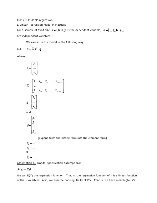
Class 3: Multiple regressionI. Linear Regression Model in Matrices For a sample of fixed size y n i,,1 is the dependent variable; 11,,1 p x x Xare independent variables. We can write the model in the following way:(1) X y ,wheren y y y (1))1()1(1211211...1......1p n p n n x x x x x x Xn (1)and110....p[expand from the matrix form into the element form]Assumption A0 (model specification assumption):X y R )(We call R(Y) the regression function. That is, the regression function of y is a linear function of the x variables. Also, we assume nonsingularity of X'X . That is, we have meaningful X 's..........21 n y y yII. Least Squares Estimator in Matrices Pre-multiply (1) by X ' (2),'''1 X X X y X pAssumption A1 (orthogonality assumption): we assume that is uncorrelated with each and every vector in X . That is,(3).0)(0),(0)(0),(0)(0),(0)(112111 p p x E x Cov x E x Cov x E x Cov ESample analog of expectation operator is n1. Thus, we have(4)01010101)1(21 i p i i i i i i x nx n x n n That is, there are a total of p restriction conditions, necessary for solving p linear equations to identify p parameters. In matrix format, this is equivalent to:(5).][or,][1o X o X nSubstitute (5) into (2), we have (6))()(X X y XThe LS estimator is then:(7),)(1y X X X bwhich is the same as the least squares estimator. Note: A1 assumption is needed for avoiding biases. III. Properties of the LS Estimator For the mode X y ,A1]using result, [important ][)(][)(])[(])[()]()[(])[()()(1111111o X E X X E X X X X X X X E X X X X E X X X X E y X X X E b E y X X X bthat is, b is unbiased.V (b ) is a symmetric matrix, called variance and covariance matrix of b .)(......)...(),(...),()()(1110100p b V b V b b Cov b b Cov b V b V 1111111)(][)()on al (condition ])[()])()[()]()[(])[()( X X X V X X X X X X X V O X X X X X X X V X X X X V y X X X V b V(after assuming I V 2][ non-serial correlation and homoscedasticity)21)( X X [important result, using A2][blackboard ]22001. Assumption A2 (iid assumption): independent and identically distributed errors. Two implications:1. Independent disturbances, j i E j i ,0),(Obtaining neat v (b ).2. Homoscedasticity, j i v E i j i ,)()(2Obtaining neat v (b ).I V 2)( , scalar matrix.IV. Fitted Values and Residualsy H y X X X X b X y 1)(ˆ X X X X H n n 1)(is called H matrix, or hat matrix. H is an idempotent matrix:H HHFor residuals:y H I y H y yy e )(ˆ (I-H ) is also an idempotent matrix.V. Estimation of the Residual Variance A. Sample Analog (8))()]([)(222i i i i E E E Vis unknown but can be estimated by e , where e is residual. Some of you may have noticedthat I have intentionally distinguished from e . is called disturbance, and e is called residual. Residual is defined by the difference between observed and predicted values.The sample analog of (8) is2)1()1(2211022)]([1)ˆ(11 p i p i i i i i i x b x b x b b y ny y n e nIn matrix:e e e i 2The sample analog is thenn e e /B. Degrees of FreedomAs a general rule, the correct degrees of freedom equals the number of totalobservations minus the number of parameters used in estimation.In multiple regression, there are p parameters to be estimated. Therefore, theremaining degrees of freedom for estimating disturbance variance is n-p . C. MSE as the EstimatorMSE is the unbiased estimator. It is unbiased because it corrects for the loss ofdegrees of freedom in estimating the parameters.ee p n MSE e pn MSE i112D. Statistical InferencesNow that we have point estimates (b ) and the variance-covariance matrix of b . But wecannot do formal statistical tests yet. The question, then, is how to make statistical inferences, such as testing hypotheses and constructing confidence intervals. Well, the only remaining thing we need is the ability to use some tests, say t , Z , or F tests.Statistical theory tells us that we can conduct such tests if e is not only iid, but iid in anormal distribution. That is, we assumeAssumption A3 (normality assumption): i is distributed as ),0(2NWith this assumption, we can look up tables for small samples.However, A3 is not necessary for large samples. For large samples, central limit theoryassures that we can still make the same statistical inferences based on t, z , or F tests if the sample is large enough.A Summary of Assumptions for the LS Estimator 1. A0: Specification assumptionX X y )|(EIncluding nonsingularity of X X .Meaningful X 's.With A0, we can computey X X X b 1)(2. A1:orthoganality assumption0)(k x E , for k = 0, .... p-1, x 0 = 1.Meaning: 0)( E is needed for the identification of 0 .All other column vectors in X are orthogonal with respect to .A1 is needed for avoiding biases. With A1, b is unbiased and consistent estimator of . Unbiasedness means that)(b EConsistency: n b as .For large samples, consistency is the most important criterion for evaluating estimators.3. A2. iid independent and identically distributed errors. Two implications:1. Independent disturbances, j i Cov j i ,0),(Obtaining neat v(b).2. Homoscedasticity, j i v Cov i j i ,)(),(2Obtaining neat v(b).I V 2)( , scalar matrix.With A2, b is an efficient estimator.Efficiency: an efficient estimator has the smallest sampling variance among all unbiased estimators. That is),ˆ()(Var somehow b Var whereˆ denotes any unbiased estimator. Roughly, for efficient estimators, imprecision [i.e., SD(b )] decreases by the inverse of the square root of n . That is, if you wish to increase precision by 10 times, (i.e., reduce S.E. by a factor of ten), you would need to increase the sample size by 100 times.A1 + A2 make OLS a BLUE estimator, where BLUE means the best, linear, unbiased estimator. That is, no other unbiased linear estimator has a smaller sampling variance than b .This result is called "Gauss-Markov theorem."4. A3. Normality, i is distributed as ),0(2NInferences: looking up tables for small samples.A1 + A2 + A3 make OLS a maximum likelihood (ML) estimator. Like all other ML estimators, OLS in this case is BUE (best unbiased estimator). That is, no other unbiased estimator can have a smaller sampling variance than OLS.Note that ML is always the most efficient estimator among all unbiased estimators. The cost of ML is really the requirement of we know the true parametric distribution of the residual. If you can afford the assumption, ML is always the best. Very often, we don't make the assumption because we don't know the parametric family of the disturbance. In general, the following tradeoff is true:More information == more efficiency. Less assumption == less efficiency.It is not correct to call certain models OLS models and other ML models. Theoretically, a same model can be estimated by OLS or ML. Model specification is different from estimation procedure.VI. ML for linear model under normality assumption (A1+A2+A3) , i :i :d N(0， 2), i = 1, … nObservations y i are independently distributed as y i ~ N(x i ’ 2); i = 1, … nUnder the normal errors assumption, the joint pdf of y’s isL = f (y 1…y n | 2) = ∏ f (y i | 2)= (2π 2)-n/2 exp{-(2 2)-1∑(y i - x i ’ }Log transformation is a monotone transformation. Maximizing L is equivalent to maximizing logL below:l = logL = (-n/2) log(2π 2) - (2 2)-1 ∑(y i - x i ’It is easy to see that what maximizes l (Maximum Likelihood Estimator) is the same as the LS estimator.。

北大暑期课程《回归分析》(Linear Regression Analysis)讲义PKU6

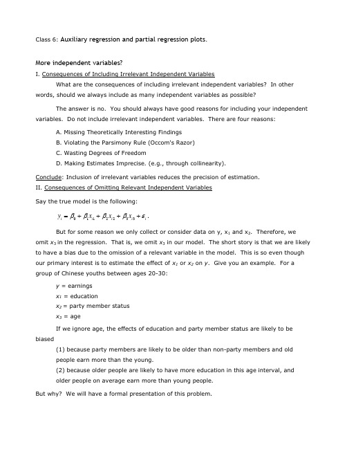
Class 6: Auxiliary regression and partial regression plots.More independent variables?I. Consequences of Including Irrelevant Independent VariablesWhat are the consequences of including irrelevant independent variables? In otherwords, should we always include as many independent variables as possible?The answer is no. You should always have good reasons for including your independentvariables. Do not include irrelevant independent variables. There are four reasons:A. Missing Theoretically Interesting FindingsB. Violating the Parsimony Rule (Occom's Razor)C. Wasting Degrees of FreedomD. Making Estimates Imprecise. (e.g., through collinearity).Conclude: Inclusion of irrelevant variables reduces the precision of estimation. II. Consequences of Omitting Relevant Independent Variables Say the true model is the following: i i i i i x x x y εββββ++++=3322110.But for some reason we only collect or consider data on y, x 1 and x 2. Therefore, weomit x 3 in the regression. That is, we omit x 3 in our model. The short story is that we are likely to have a bias due to the omission of a relevant variable in the model. This is so even though our primary interest is to estimate the effect of x 1 or x 2 on y . Give you an example. For a group of Chinese youths between ages 20-30: y = earnings x 1 = educationx 2 = party member status x 3 = ageIf we ignore age, the effects of education and party member status are likely to be biased(1) because party members are likely to be older than non-party members and old people earn more than the young.(2) because older people are likely to have more education in this age interval, and older people on average earn more than young people.But why? We will have a formal presentation of this problem.III: Empirical Example of Incremental R-SquaresXie and Wu’s (2008, China Quarterly) study of earnings inequality in three Chinese cities: Shanghai, Wuhan, and Xi’an in 1999. See the following tables:Variables DF R2∆R2(1) ∆R2(2)City 2 17.47 *** 18.11 *** 19.12 *** Education Level 5 7.82 *** 5.49 *** 4.46 *** Experience+Experience2 2 0. 23 0.17 0.05 Gender 1 4.78 *** 4.84 *** 3.05 *** Cadre Status 1 3.08 *** 2.27 *** 0.63 *** Sector 3 3.54 *** 2.18 *** 1.80 *** Danwei Profitability(linear) 1 12.52 *** 9.30 *** Danwei Profitability(dummies) 4 12.89 ***N = 1771Note: DF refers to degrees of freedom.∆R2(1) refers to the incremental R2 after the inclusion of Danwei'sfinancial situation (linear).∆R2(2) refers to the incremental R2 after the inclusion of all the other variables.*** p< 0.001, ** p<0.01, * p<0.05, based on F-tests.Source: 1999 Three-City Survey.Table 2: Estimated Regression Coefficients on Logged EarningsVariables Observed Effects Adjusted Effects β SE(β) β SE(β)City (Shanghai=excluded)-0.465 *** 0.033 -0.539 *** 0.028 Xi’an-0.628 *** 0.034 -0.658 *** 0.028 Constant 9.402 *** 0.024Education Level (no schooling=excluded)Primary 0.536 * 0.216 0.414 * 0.170 Junior high 0.737 *** 0.202 0.447 ** 0.161 Senior high 0.770 *** 0.201 0.592 *** 0.161 Junior college 1.049 *** 0.203 0.778 *** 0.162 College 1.253 *** 0.207 0.923 *** 0.166 Constant 8.120 *** 0.210Experience+Experience2-11.235 6.029 2.421 4.775 Experience2 (x1000) 0.288 * 0.144 -0.017 0.114 Constant 9.113 *** 0.059Gender (male=excluded)Female -0.276 *** 0.029 -0.225 *** 0.023 Constant 9.144 *** 0.019Cadre Status (non-cadre=excluded)0.375 *** 0.050 0.185 *** 0.042 Constant 8.992 *** 0.015Sector (government+public=excluded)State owned -0.133 *** 0.037 -0.043 0.030 Collectively owned -0.397 *** 0.057 -0.224 *** 0.045 Privately owned 0.027 0.047 0.114 ** 0.037 Constant 9.129 *** 0.031Danwei Profitability (linear) 0.256 *** 0.016 0.227 *** 0.013 Constant 8.270 *** 0.050Danwei Profitability (dummies)(very poor=excluded)Relatively poor 0.100 0.062Average 0.405 *** 0.054Fairly good 0.702 *** 0.059Very good 0.918 *** 0.108Constant 8.624 *** 0.050Constant 8.237 *** 0.171 R2 (N = 1771)43.92%Note: Observed effects on logged earnings are derived from bivariate models. Adjusted effects are derived from a multivariate model including all variables.*** p< 0.001, ** p<0.01, * p<0.5, based on two-sided t-tests.IV. Auxiliary Regressions True regression:(1)i p i p p i p i i x x x y εββββ+++++=----)1()1()2()2(110Without loss of generality, say that 1-p x is omitted: (2)i p i p i i x x y δααα++++=--)2()2(110We can have an auxiliary regression to express the missing variable x p -1: (3)i p i p i p x x x μτττ++++=---)2()2(1101Substitute (3) into (1): (4) ii p p i p p p i p p ii p i p i p p i p i i x x x x x x y εμβτββτββτββεμτττββββ++++++++=+++++++++=------------)1()2()2()1()2(11)1(10)1(0)2()2(110)1()2()2(110)()()(Now you can see where the biases are: k p k k τββα1-+=,where k p τβ1- is called the bias. The bias is the product of the effect of the omitted variable on the dependent variable (1-p β) and the effect of the independent variable of interest on the omitted variable (k τ). Thus, there are two conditions for the existence of omitted variable bias: (1) Relevance Condition: the variable omitted is relevant, that is 0)1(≠-p β(2) Correlation Condition: the variable omitted is related to the variable of interest.[blackboard : path diagram]How does an experimental design help eliminate omitted bias? [through eliminating the correlation condition)Short of experiments, we need to include all relevant variables in order to avoid omitted variable bias.V. Criteria for Variable Inclusion and ExclusionA. Theoretical Reasoning for InclusionB. F-Tests to Exclude Irrelevant Variables: A Review Do not exclude variables on the basis of F-tests alone. Both theoretical reasoning andF-tests should be used.VI. Partial Regression Estimation True regression:i p i p i i x x y εβββ++++=--)1()1(110....In matrix:εβ+=X yThis model can always be written into: (1)1122y X X ββε=++where now []⎥⎦⎤⎢⎣⎡==2121,βββX X X21X and X are matrices of dimensions )(,2121p p p p n p n =+⨯⨯ and 21ββ+are parametervectors, of dimensions 21,p p .We first want to prove that regression equation (1) is equivalent to the following procedure: (1) Regress1on X y , obtain residuals *y ;(2) Regress 12on X X , obtain residuals *2X ;(3) Then regress *y on *2X , and obtain the correct least squares estimates of 2β(=2b ), sameas those from the one-step method.This is an alternative way to estimate 2β. Note that we do not obtain estimates for 1β in thisway. Proof:pre-multiply (1) by ')'(11111X X X X -:(1H hat matrix based on X 1; ).')'( call us let 111111X X X X H -=(2)εββ')'(')'(')'(')'(111112211111111111111111X X X X X X X X X X X X X X y X X X X ----++= (The last term is zero by assumption), thus (3)221111ββX H X y H +=Now (1)-(3):εβ+-+=-2211)(0)(X H I y H I(4)εβ+=22**X y .Therefore, the estimation of 2βfrom (4) should be identical to the estimation of 2βfrom (1). This is always true: three-step estimation of partial regression coefficients.Note the same residual term ε appears in (4) as in (1). Interpretation:(1) purge y of linear combinations of *1y ⇒X . (2) purge 2X of linear combinations of *21X ⇒X(3) regress y * on 2X *, noting that both y* and 2X * are purged of the confounding effects of X 1.Note: 2X in general can be a matrix, i.e., contains more than one independent variable. Regress one column in 2X at a time, until all columns are regressed on 1X .Note that the degrees of freedom for MSE from the last step is not correct. This is the only thing that needs to be adjusted for manually. DF for MSE = n-p (instead of n-p 2)This is an important result. It was on my preliminary exam. Unfortunately, it is often neglected (even in textbooks).VII. Partial Regression Plots (Added Variable Plots)We now focus on one (and only one) particular independent variable and wish to see its effect while controlling for other independent variables. A. Based on "Partial Regression Estimation" with 3 steps:We divide X into two parts: X -k + x k1. Regress y on X -k , obtain residuals called y*2. Regress x k on X -k , obtain residuals called x k *3. Regress y* on x k* gives the true partial regression coefficient of x k.Definition: A plot between y* and x k* is called a partial regression plot or an added-variable plot.Question: what is different between the three-stage partial regression method and a one-step multiple regression?Point estimate: the sameResiduals: the sameMSE: different because it is necessary to adjust the degrees of freedom: n-p instead of n-1.Therefore, you cannot use the computer output directly for any statistical inference if you do a 3-step partial regression estimation.B. Sum of Squares from the Partial Regression PlotsVIII. Illustration with an example:Model Description SSE DF SSE1 y on 1, x1, x2SSE1n-32 y on 1, x1⇒ y* SSE2n-23 x2 on 1, x1⇒ x2* SSE3n-24 y* on x2* SSE4n-3Note: SSE4 = SSE1; DE SSE4 = DE SSE1For example, if we only know Models 2 and 4, can we test the hypothesis that x2 has no effect after x1 is controlled?Yes. We can nest Models 2 and 4:F1, n-3 = (SSE2 - SSE4)/(SSE4/(n-3)).C. Examplesy = incomex1 = sexx2 = abilityn=100Model Description SSE DF SSE R2 SST1 y on 1, x1, x230 [97] .70 SST=1002 y on 1, x1⇒ y* 60 [98] [.40]3 x2 on 1, x1⇒ x2* 4000 [98] 0.60 SST=10000Reported4a y* on x2* 30 [99] [0.50] *ImportantMeaningful4b y* on x2* 30 [97] [0.70]Test the hypothesis that x2 has no partial effect after controlling for x1 even if we do not run Model 1:Nesting Models 2 and 4b:F = (60 - 30)/(30/97) = 30/0.31 = 96.77, significant.。

北大暑期课程回归分析

北大暑期课程《回归分析》(Linear-Regression-Analysis)讲义pku4说课材料

Class 4: Inference in multiple regression.I. The Logic of Statistical InferenceThe logic of statistical inference is simple: we would like to make inferences about a population from what we observe from the sample that has been drawn randomly from the population.The samples' characteristics are called "point estimates."It is almost certain that the sample's characteristics are somewhat different from the population's characteristics. But because the sample was drawn randomly from the population, the sample's characteristics cannot be "very different" from thepopulation's characteristics. What do I mean by "very different"? To answer this question, we need a distance measure (or dispersion measure), called the standard deviation of the statistic.To summarize, statistical inferences consist of two steps:(1) Point estimates (sample statistics) (2) Standard deviations of the point estimates (dispersion of sample statisticsin a hypothetical sampling distribution).II. Review: For a sample of fixed size y n i ,,1 is the dependent variable;11,,1 p x x X contains independent variables.We can write the model in the following way: , X yUnder certain assumptions, the LS estimator 1()b X X X yAs certain desirable properties:A1 => unbiasedness and consistency A1 + A2 => BLUE, with 12()()V b X XA1 + A2 + A3 =>BUE 12()()V b X X(even for small samples)III. The Central Limit Theorem Statement: The mean of iid random variables (with mean of , and variance of 2 ) approaches a normal distribution as the number of random variables increases. n n N X n as ),/,(2The property belongs to the statistic -- sample mean in the sampling distribution of all sample means, even though the random variables themselves are not normally distributed. You can never check this normality because you can only have one sample statistic.In regression analysis, we do not assume that is normally distributed if we have a large sample, because all estimated parameters approach to normal distributions. Why: all LS estimates are linear function of (proved last time). Recall a theorem: a linear transformation of a variable distributed as normal is also distributed as normal.IV. Inferences about Regression CoefficientsA. Presentation of Regression ResultsCommon practice: give a star beside the parameter estimate for significance level of 0.05, two stars for 0.01, and three stars for 0.001. For example: Dependent Variable: EarningsIndependent Variable:Father's education 0.900*Mother's education 0.501***Shoe size -2.16What is the problem with this practice?First, we want to have a quantitative evaluation of the significance level. We should not blindly rely on statistical tests. For example,Father's education 0.900* (0.450)Mother's education 0.501*** (0.001)Shoe size -2.16 (1.10)In this case, is father's education much more significant than shoe size? Not really. They are very similar. By contrast, mother's is far more significant than the other two.A second practice is to report the t or z values:Coeffi. t.Father's education 0.900 2.0Mother's education 0.501 500.Shoe size -2.16 -1.96This solution is much better. However, very often, our hypothesis is not about deviation from zero, but from other hypothetical values. For example, we are interested in the hypothesis whether a one-year increase in father's education will increase son's education by one year. The hypothesis here is 1 instead of 0.The preferred way of presentation is: Coeff.(S.E.) Father's education 0.900(0.450) Mother's education 0.501(0.001) Shoe size-2.16 (1.10) B. Difference between Statistical Significance and the Size of an EffectStatistical significance always refers to a stated hypothesis. You will see a lot of misuses in the literature, sometimes by well-known sociologists. They would saythat this variable is highly significant. That one is not significant. This is not correct. I am not responsible for their mistakes, but I want to warn you not to commit the same mistakes again. In our example, you could say Mother's education is highly significant from zero. But it is not significant from 0.5. Had your hypothesis been that the parameter for Mother's education is 0.5, the result would be consistent with the hypothesis. That is, statistical significance should always be made with reference to a hypothesis. Follow2/)(022b SE b z Another common mistake is to equate statistical significance with the size of an effect. A variable can be statistically significant from zero. But the estimated coefficient is small. The contribution of father's education to the dependent variable is larger than that of mother's education even though mother's education is more statistically significant from zero than father's education.Important: you should look at both coefficients and their standard errors.C. Confidence Intervals for Single Parameters)(96.1j j j b SE bD. Hypothesis Testing for Single ParametersCompare )(/)(0j j j b SE b z , if z is outside the range of -1.96 and 1.96, the hypothesis is rejected. Otherwise, we fail to reject the hypothesis.V. Inferences about Linear Combinations of Two ParametersExample 1: 21(equality hypothesis), ==> 021Example 2: 2110 (proportionality hypothesis), ==>01021Example 3: 221(surplus hypothesis), ==> 221In general form, we may have )(2211 c cHypothesis testing:c c c 2211 Confidence interval:2211 c c lies between (low limit, upper limit)Procedure:A. Point estimate:Compute 2211b c b cB. Degree of Imprecision),(2)()()(21212221212211b b Cov c c b V c b V c b c b c V and then take square root of )(2211b c b c V .We would need to obtain the variance-covariance matrix of the parameter vector in order to carry out the calculation.)( and )(21b V b V are on the diagonal,),(21b b Cov is off-diagonal.Let us look at the first half the example. Compute the confidence interval for the hypothesis that 1= 2.Step 1. b 1 - b 2 = 5732.0- 3146.0 = 0.2586.Step 2: V(b 1 - b 2) = 0642.0+ 0310.0-2* (0227.0 ) = 0.1406.SD(b 1 - b 2) = 0.14061/2 = 0.3750.Step 3:Computet 2 = (0.2586 -0)/ 0.3750 = 0.6897, insignificant (unsurprising result).Note DF = 5-3 = 2.I use two parameters as an example.Examples of Hypothesis Testing:Example 1: 21 (equality hypothesis), ==>021Example 2: 2110 (proportionality hypothesis), ==>01021Example 3: 221 (surplus hypothesis), ==>221In general form,We may have c c 2211Hypothesis testing: c c c 2211Confidence interval: 2211c c lies between (low limit, upper limit)Procedure:A. Find point estimate:Compute 1c 1b +2c 2bB. Find degree of Imprecision 21212221212211b ,b Cov c c 2b V c b V c b c b c V and then take square root of 2211b c b c V .We would need to obtain the variance-covariance matrix of the parameter vector in order to carry out the calculation.V(1b ) and V(2b ) are on the diagonal,Cov(1b ,2b ) is off-diagonal.Numerical Example: Multiple regressions For the following small data set (n = 5), use matrix operations to solve the following problems. You should make use of the information below as much as possible. Let65420',40201',42301',12121x x y x xIt is known that813271775'4610'y0582.0426.1381.0426.1205.0239.1381.0239.7030.)'(11. Write out X and y in full. 1112212231324142515211101110201,12431105211464x x x x x x y x x x x2. Write X X and y X in full.57171072132,2317328146X X X y3. Estimate b with the help of a calculator (b is the least squares estimator of , theregression coefficients of X ).10.703 -0.024 -0.138 100.128 (')'-0.024 0.120 -0.043 230.573 -0.138 -0.043 0.058 460.315 b X X X y4. Find the predicted values for y . $0.701 1100.128 0.757 1020.573 2.533 1240.315 1.701 105 4.308 146y X b5. Calculate SST, SSR, and SSE. (Hint: to obtain SSR, you may use the results from 4. µµ222222222222222222222222222()(12)(02)(32)(22)(42)10103245210()(0.7012)(0.7572)(2.5332)(1.7012)(4.3082)8.9350.7010.757 2.533 1.701 4.308i i i i SST Y Y Y nY SSR YY Y nY 8.935108.935 1.065SSE SST SSR6. Calculate the variance-covariance matrix of b .1110.703 -0.024 -0.138 0.375 -0.013 -0.074 1.065()(')'()(')(')-0.024 0.120 -0.043 -0.013 0.064 -0.023 53-0.138 -0.043 0.058 -0.074 -0.023 0.031 V b X X X V e X X X X X MSE。

1、下载文档前请自行甄别文档内容的完整性，平台不提供额外的编辑、内容补充、找答案等附加服务。
2、"仅部分预览"的文档,不可在线预览部分如存在完整性等问题,可反馈申请退款(可完整预览的文档不适用该条件!)。
3、如文档侵犯您的权益，请联系客服反馈,我们会尽快为您处理(人工客服工作时间：9:00-18:30)。

Class 5: ANOVA (Analysis of Variance) and F-testsI. What is ANOVAWhat is ANOVA? ANOVA is the short name for the Analysis of Variance. The essenceof ANOVA is to decompose the total variance of the dependent variable into two additive components, one for the structural part, and the other for the stochastic part, of a regression. Today we are going to examine the easiest case.II. ANOVA: An IntroductionLet the model beεβ+= X y .Assuming x i is a column vector (of length p) of independent variable values for the i th'observation,i i i εβ+='x y .Then b 'x i is the predicted value.sum of squares total:[]∑-=2Y y SST i []∑-+-=2'x b 'x y Y b i i i[][][][]∑∑∑-+-+-=Y -b 'x b 'x y 2Y b 'x b 'x y 22i i i i i i[][]∑∑-+=22Y b 'x e i ibecause [][][]∑∑=-=--0Y b 'x e Y b 'x b 'x y ii i i i .This is always true by OLS. = SSE + SSRImportant: the total variance of the dependent variable is decomposed into two additive parts: SSE, which is due to errors, and SSR, which is due to regression. Geometric interpretation: [blackboard ]Decomposition of VarianceIf we treat X as a random variable, we can decompose total variance to the between-group portion and the within-group portion in any population:()()()i i i x y εβV 'V V +=Prove:()()i i i x y εβ+='V V()()()i i i i x x εβεβ,'Cov 2V 'V ++=()()iix εβV 'V +=(by the assumption that ()0 ,'Cov =εβk x , for all possible k.)The ANOVA table is to estimate the three quantities of equation (1) from the sample.As the sample size gets larger and larger, the ANOVA table will approach the equation closer and closer.In a sample, decomposition of estimated variance is not strictly true. We thus need toseparately decompose sums of squares and degrees of freedom. Is ANOVA a misnomer?III. ANOVA in MatrixI will try to give a simplied representation of ANOVA as follows:[]∑-=2Y y SST i ()∑-+=i i y Y 2Y y 22∑∑∑-+=i i y Y 2Y y 22∑-+=222Y n 2Y n y i (because ∑=Y n y i )∑-=22Y n y i2Y n y 'y -=y J 'y n /1y 'y -= (in your textbook, monster look)SSE = e'e[]∑-=2Y b 'x SSR i()()[]∑-+=Y b 'x 2Y b 'x 22i i()[]()∑∑-+=b 'x Y 2Y n b 'x 22i i()[]()∑∑--+=i i i e y Y 2Y n b 'x 22()[]∑-+=222Y n 2Y n b 'x i(because ∑∑==0e ,Y n y i i , as always)()[]∑-=22Yn b 'x i2Y n Xb X'b'-=y J 'y n /1y X'b'-= (in your textbook, monster look)IV. ANOVA TableLet us use a real example. Assume that we have a regression estimated to be y = - 1.70 + 0.840 xANOVA TableSOURCE SS DF MS F with Regression 6.44 1 6.44 6.44/0.19=33.89 1, 18Error 3.40 18 0.19 Total 9.8419We know∑=100xi, ∑=50y i , 12.509x 2=∑i , 84.134y 2=∑i , ∑=66.257y x i i . If weknow that DF for SST=19, what is n?n= 205.220/50Y ==84.95.25.22084.134Y n y SST 22=⨯⨯-=-=∑i()[]∑-+=0.1250.84x 1.7-SSR 2i[]∑-⨯⨯⨯-⨯+⨯=0.125x 84.07.12x 84.084.07.17.12i i= 20⨯1.7⨯1.7+0.84⨯0.84⨯509.12-2⨯1.7⨯0.84⨯100- 125.0= 6.44SSE = SST-SSR=9.84-6.44=3.40DF (Degrees of freedom): demonstration. Note: discounting the intercept when calculating SST. MS = SS/DFp = 0.000 [ask students]. What does the p-value say?V. F-TestsF-tests are more general than t-tests, t-tests can be seen as a special case of F-tests.If you have difficulty with F-tests, please ask your GSIs to review F-tests in the lab. F-tests takes the form of a fraction of two MS's.MS R/MS E F , df2df1An F statistic has two degrees of freedom associated with it: the degree of freedom inthe numerator, and the degree of freedom in the denominator.An F statistic is usually larger than 1. The interpretation of an F statistics is thatwhether the explained variance by the alternative hypothesis is due to chance. In other words, the null hypothesis is that the explained variance is due to chance, or all the coefficients are zero.The larger an F-statistic, the more likely that the null hypothesis is not true. There is atable in the back of your book from which you can find exact probability values.In our example, the F is 34, which is highly significant.VI. R 2R 2 = SSR / SSTThe proportion of variance explained by the model. In our example, R-sq = 65.4%VII. What happens if we increase more independent variables.1. SST stays the same.2. SSR always increases.3. SSE always decreases.4. R 2 always increases.5. MSR usually increases.6. MSE usually decreases.7. F-test usually increases.Exceptions to 5 and 7: irrelevant variables may not explain the variance but take up degrees of freedom. We really need to look at the results.VIII. Important: General Ways of Hypothesis Testing with F-Statistics.All tests in linear regression can be performed with F-test statistics. The trick is to run"nested models."Two models are nested if the independent variables in one model are a subset or linearcombinations of a subset （子集）of the independent variables in the other model.That is to say. If model A has independent variables (1, 1x , 2x ), and model B hasindependent variables (1, 1x , 2x ,3x ), A and B are nested. A is called the restricted model; B is called less restricted or unrestricted model. We call A restricted because A implies that0=3β. This is a restriction.Another example: C has independent variable (1, 1x , 2x +3x ), D has (1, 2x +3x ). C and A are not nested.C and B are nested. One restriction in C: 32ββ= . C and D are nested. One restriction in D: 0=1β.D and A are not nested.D and B are nested: two restriction in D: 32ββ=; 0=1β.We can always test hypotheses implied in the restricted models. Steps: run tworegression for each hypothesis, one for the restricted model and one for the unrestrictedmodel. The SST should be the same across the two models. What is different is SSE and SSR. That is, what is different is R 2. Let()()df df SSE ,df df SSE u u r r ==; df df ()()0u r u r r u n p n p p p -=---=-<Use the following formulas:()()()()(),SSE SSE /df SSE df SSE F SSE /df r u r u dfr dfu dfu u u---=or()()()()(),SSR SSR /df SSR df SSR F SSE /df u r u r dfr dfu dfu u u---=(proof: use SST = SSE+SSR)Note, df(SSE r )-df(SSE u ) = df(SSR u )-df(SSR r ) =df ∆,is the number of constraints (not number of parameters) implied by the restricted modelor()()()22,2R R /df F 1R /dfur dfr dfu dfuuu--∆=- Note thatdf 1df ,2F t =That is, for 1df tests, you can either do an F-test or a t-test. They yield the same result. Another way to look at it is that the t-test is a special case of the F test, with the numerator DF being 1.IX. Assumptions of F-testsWhat assumptions do we need to make an ANOVA table work?Not much an assumption. All we need is the assumption that (X'X) is not singular, so that the least square estimate b exists.The assumption of ε'X =0 is needed if you want the ANOVA table to be an unbiased estimate of the true ANOVA (equation 1) in the population. Reason: we want b to be an unbiased estimator of β, and the covariance between b and εto disappear.For reasons I discussed earlier, the assumptions of homoscedasticity and non-serial correlation are necessary for the estimation of ()i Vε.The normality assumption that εi is distributed in a normal distribution is needed for small samples.X. The Concept of IncrementEvery time you put one more independent variable into your model, you get an increase in 2R . We sometime called the increase "incremental 2R ." What is means is that more variance is explained, or SSR is increased, SSE is reduced. What you should understand is that the incremental 2R attributed to a variable is always smaller than the 2R when other variables are absent.XI. Consequences of Omitting Relevant Independent VariablesSay the true model is the following:0112233i i i i i y x x x ββββε=++++.But for some reason we only collect or consider data on21,,x and x y . Therefore, we omit3x in the regression. That is, we omit in 3x our model. We briefly discussed this problembefore. The short story is that we are likely to have a bias due to the omission of a relevant variable in the model. This is so even though our primary interest is to estimate the effect of1x or 2x on y.Why? We will have a formal presentation of this problem.XII. Measures of Goodness-of-FitThere are different ways to assess the goodness-of-fit of a model. A. R 2R 2 is a heuristic measure for the overall goodness-of-fit. It does not have an associated test statistic.R 2 measures the proportion of the variance in the dependent variable that is “explained” by the model: R 2 =SSESSR SSRSST SSR +=B. Model F-testThe model F-test tests the joint hypotheses that all the model coefficients except for the constant term are zero.Degrees of freedoms associated with the model F-test: Numerator: p-1 Denominator: n-p.C. t-tests for individual parametersA t-test for an individual parameter tests the hypothesis that a particular coefficient is equal to a particular number (commonly zero).t k = (b k - βk0)/SE k , where SE k is the (k, k) e lement of MSE(X’X)-1, with degree of freedom=n-p. D. Incremental R 2Relative to a restricted model, the gain in R 2 for the unrestricted model: ∆R 2= R u 2- R r 2E. F-tests for Nested ModelIt is the most general form of F-tests and t-tests.()()()()(),SSE SSE /df SSE df SSE F SSE /df r u r dfu dfr u dfu u u---=It is equal to a t-test if the unrestricted and restricted models differ only by one single parameter.It is equal to the model F-test if we set the restricted model to the constant-only model.[Ask students] What are SST, SSE, and SSR, and their associated degrees of freedom, for the constant-only model?Numerical ExampleA sociological study is interested in understanding the social determinants of mathematicalachievement among high school students. You are now asked to answer a series of questions. The data are real but have been tailored for educational purposes. The total number of observations is 400. The variables are defined as: y: math scorex1: father's education x2: mother's educationx3: family's socioeconomic status x4: number of siblings x5: class rankx6: parents' total education (note: x6 = x1 + x2) For the following regression models, we know: Table 1 SST SSR SSE DF R 2 (1) y on (1 x1 x2 x3 x4) 34863 4201 (2) y on (1 x6 x3 x4) 34863 396 .1065 (3) y on (1 x6 x3 x4 x5) 34863 10426 24437 395 .2991 (4) x5 on (1 x6 x3 x4) 269753 396 .02101. Please fill the missing cells in Table 1.2. Test the hypothesis that the effects of father's education (x1) and mother's education (x2) on math score are the same after controlling for x3 and x4.3. Test the hypothesis that x6, x3 and x4 in Model (2) all have a zero effect on y.4. Can we add x6 to Model (1)? Briefly explain your answer.5. Test the hypothesis that the effect of class rank (x5) on math score is zero after controlling for x6, x3, and x4.Answer: 1. SST SSR SSE DF R 2 (1) y on (1 x1 x2 x3 x4) 34863 4201 30662 395 .1205 (2) y on (1 x6 x3 x4) 34863 3713 31150 396 .1065 (3) y on (1 x6 x3 x4 x5) 34863 10426 24437 395 .2991 (4) x5 on (1 x6 x3 x4) 275539 5786 269753 396 .0210Note that the SST for Model (4) is different from those for Models (1) through (3). 2.Restricted model is 01123344()y b b x x b x b x e =+++++Unrestricted model is ''''''011223344y b b x b x b x b x e =+++++(31150 - 30662)/1F 1,395 = -------------------- = 488/77.63 = 6.29 30662 / 395 3.3713 / 3F 3,396 = --------------- = 1237.67 / 78.66 = 15.73 31150 / 3964. No. x6 is a linear combination of x1 and x2. X'X is singular.5.(31150 - 24437)/1F 1,395 = -------------------- = 6713 / 61.87 = 108.50 24437/395t = 10.42t ===。