Mining high-speed data streams
frequent造句
frequent造句1、Willing to have frequent travel.愿意经常出差。
2、ordinariness as a consequence of being frequent and commonplace频繁发生,经常见到。
3、a person you come to know by by frequent friendly correspondence.通过经常地友好交流相互了解的人。
4、One of the least frequent is the congregational form so familiar in the West.其中最频繁的是公理的形式非常熟悉在西方。
5、Constant and frequent retrieval of the same redundant data.频繁地检索相同的冗余数据。
6、The best ornament of a house is the friends who frequent it常来造访的朋友是房子最好的装饰。
7、Research on Aggregation Query and Mining Frequent Patterns in Data Streams数据流聚集查询和频繁模式挖掘的研究8、Nearby, residents frequent posh bars, art galleries and high-end restaurants.附近有不少豪华的酒吧、画廊与高级餐厅。
9、Second-line agents were used for steroid dependence, steroid resistance, or frequent relapses. 二线的药物被用于激素依赖型、激素抵抗型和频繁复发者。
10、Ocular symptoms are a frequent presenting chief complaint from patients in the outpatient setting.在门诊中经常可以遇到以眼部症状为主诉的病人。
亚马逊雨林简介英语作文

Amazon Rainforest IntroductionNestled deep within the heart of South America, the Amazon Rainforest stands as a veritable green lung of the planet, exhaling life and vitality. Spanning across nine countries and covering a vast area of over six million square kilometers, it is the largest tropical rainforest in the world, harboring an incredibly diverse array of plant and animal species.The Amazon Rainforest is renowned for its biodiversity, boasting over half of the world's known plant species and tens of thousands of animal species, many of which are yet to be discovered or fully understood. From towering mahogany trees to intricate orchids, and from elusive jaguars to colorful parrots, the rainforest is a living museum of natural history.The climate of the Amazon Rainforest is tropical, with high temperatures and heavy rainfall throughout the year. This wet and warm environment is conducive to the growth of lush vegetation, creating a dense canopy that shields the forest floor from direct sunlight. The resulting layers ofthe rainforest - the emergent, canopy, understory, and forest floor - each support their own unique ecosystems.The Amazon River, the lifeblood of the rainforest, flows through its heart, nurturing the rich biodiversity. Its tributaries and streams form a complex network that spreads across the entire rainforest, providing water and nutrients to the surrounding ecosystems.However, the Amazon Rainforest is facing numerous threats. Deforestation, driven by the demands of agriculture, logging, and mining, has led to significant losses of forest cover. Climate change is also having a profound impact, altering rainfall patterns and increasing the frequency of extreme weather events. These threats pose a significant challenge to the conservation of the rainforest's biodiversity and ecological balance.Despite these challenges, efforts are being made to protect the Amazon Rainforest. Conservation organizations, governments, and local communities are working together to implement sustainable practices and policies that aim to reduce deforestation and promote the preservation of the rainforest's natural resources.In conclusion, the Amazon Rainforest is a priceless treasure trove of biodiversity and ecological wisdom. It is not only a vital source of natural resources but also a crucial component of the global ecological system. Its protection and preservation are essential for safeguarding the health of our planet and ensuring a sustainable future for all.**亚马逊雨林简介**亚马逊雨林深藏于南美洲的心脏地带,宛如地球的绿色肺腑,散发着生命与活力。
Oracle各版本区别
Oracle各版本区别Oracle EE(企业版, Enterprise Edition), SE(标准版, Standard Edition), SE1(标准版1, Standard Edition One) 区别是什么?1. SE1针对部门和小企业,SE针对中小企业和单位,EE针对大中型企业和单位。
使用SE,就意味着用户不能使用EE的功能强大的选件,EE选件可以实现高性能、高可用性、高扩展性、高安全性和高级数据分析的功能。
SE和SE1最多支持 500 GB 数据量,EE则高达 8,000,000,000 GB(80亿GB),另外EE还支持数据压缩(compression)功能,特别适合存储资源有限、I/O量大的数据仓库。
2. 10g SE集群(RAC)功能有限,扩展只能到4个处理器(processor),不能使用集群文件系统(CFS)和第三方软件(如, Veritas),而且对于存储只能使用裸设备(Raw Device),不易管理。
EE没有上述限制。
3. EE支持自动故障诊断、自动调优、大规模数据库的变更管理和配置管理,降低DBA的工作强度和人为错误概率,SE不具备此功能。
4. SE适合中小数据库,只支持全备份,不支持EE所具备的增量备份(incremental backup),一个连续运行的大数据库每天做全备份是不可想像的。
EE还支持并行备份/恢复,成倍提高速度,在有限的窗口时间里完成备份/恢复,而SE没有此功能。
5. 管理用户文档的内容管理功能,SE用户必须自己开发,EE支持内容管理功能,降低用户开发成本和风险。
6. SE没有容灾功能,EE有Data Guard容灾功能,能实现远程镜像。
SE只支持单向复制(Basic Replicatio n),EE支持多主结点任意方向复制。
7. 如果从一个平台到另一个平台传输数据,SE只支持逐条记录导入、导出,比较慢。
EE支持跨平台传输表空间(Transportable tablespaces),像拷贝文件一样快;EE还支持数据仓库构建过程的数据质量控制。
Oracle EE SE SE1各版本区别

============================================================Oracle EE/SE/SE1各版本区别网络整理-王磊@2010.6.18 11:21============================================================为什么选择Oracle EE(企业版, Enterprise Edition)?简单说:EE针对大型应用系统,除数据库基本功能外,还支持系统无限扩展(scalability)、高可用性(availability)、高安全性(security)、数据分析(OLAP)、数据仓库(data warehouse)、内容管理(content management)和自动管理(auto management)功能。
适用于单机、双机、多CPU多节点集群等各种环境。
详细说:EE支持并发集群的“RAC选件”,加速大数据量访问的“分区选件”(Partitioning),多维在线分析的“OLAP选件”,预测业务发展的“数据挖掘选件”(Data Mining),管理地理信息的“空间数据选件”(Spatial),传输和存储加密的“高级安全选件”(Advanced Security),实现行级安全的“标签安全选件”(Label Security),实现内容管理的“内容数据库”和“记录数据库”(Content Database, Records Database),加强内部监控的“Database Vault”,数据仓库构建高级功能(Warehouse Builder Enterprise ETL, Warehouse Builder Data Quality),数据库自动管理功能(Enterprise Manager Packs),实现容灾的数据卫士(Data Guard),实现数据复制的流(Streams),以及支持并行执行、并行备份等。
Application_of_IRIG106_Standard_in_High-Speed_Anal
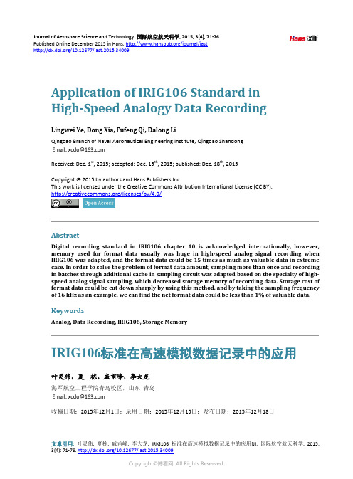
Journal of Aerospace Science and Technology 国际航空航天科学, 2015, 3(4), 71-76 Published Online December 2015 in Hans. /journal/jast /10.12677/jast.2015.34009Application of IRIG106 Standard in High-Speed Analogy Data RecordingLingwei Ye, Dong Xia, Fufeng Qi, Dalong LiQingdao Branch of Naval Aeronautical Engineering Institute, Qingdao ShandongReceived: Dec. 1st , 2015; accepted: Dec. 15th , 2015; published: Dec. 18th, 2015Copyright © 2015 by authors and Hans Publishers Inc.This work is licensed under the Creative Commons Attribution International License (CC BY). /licenses/by/4.0/AbstractDigital recording standard in IRIG106 chapter 10 is acknowledged internationally, however, memory used for format data usually was huge in high-speed analog signal recording when IRIG106 was adapted, and the format data could be 15 times as much as valuable data in extreme case. In order to solve the problem of format data amount, sampling more than once and recording in batches through additional cache in sampling circuit was adapted based on the specialty of high- speed analog signal sampling, which decreased storage memory of recording data. Storage cost of format data could be cut down sharply by using this method, and by taking the sampling frequency of 16 kHz as an example, we can find the net format data could be less than 1% of valuable data.KeywordsAnalog, Data Recording, IRIG106, Storage MemoryIRIG106标准在高速模拟数据记录中的应用叶灵伟,夏 栋,戚甫峰,李大龙海军航空工程学院青岛校区,山东 青岛收稿日期:2015年12月1日;录用日期:2015年12月15日;发布日期:2015年12月18日叶灵伟等摘要IRIG106第10章采集记录标准是国际公认的采集记录标准,但是采用IRIG106标准记录高速模拟量数据时经常存在用于存储记录格式的数据量过大的问题,极端情况下存储记录格式的数据量是有意义的记录数据量的15倍以上。
Received Revised Accepted

STRUCTURE DISCOVERY IN SEQUENTIALLY-CONNECTEDDATA STREAMSJEFFREY COBLE, DIANE J. COOK AND LAWRENCE B. HOLDERDepartment of Computer Science and EngineeringThe University of Texas at ArlingtonBox 19015, Arlington, TX 76019, USA{coble,cook,holder}@ReceivedRevisedAcceptedMuch of current data mining research is focused on discovering sets of attributes that discriminatedata entities into classes, such as shopping trends for a particular demographic group. In contrast,we are working to develop data mining techniques to discover patterns consisting of complexrelationships between entities. Our research is particularly applicable to domains in which thedata is event driven, such as counter-terrorism intelligence analysis. In this paper we describe analgorithm designed to operate over relational data received from a continuous stream. Ourapproach includes a mechanism for summarizing discoveries from previous data increments sothat the globally best patterns can be computed by examining only the new data increment. Wethen describe a method by which relational dependencies that span across temporal incrementboundaries can be efficiently resolved so that additional pattern instances, which do not resideentirely in a single data increment, can be discovered. We also describe a method for changedetection using a measure of central tendency designed for graph data. We contrast twoformulations of the change detection process and demonstrate the ability to identify salientchanges along meaningful dimensions and recognize trends in a relational data stream.Keywords: Relational Data Mining; Stream Mining, Change Detection1. IntroductionMuch of current data mining research is focused on algorithms that can discover sets of attributes that discriminate data entities into classes, such as shopping or banking trends for a particular demographic group. In contrast, our work is focused on data mining techniques to discover relationships between entities. Our work is particularly applicable to problems where the data is event driven, such as the types of intelligence analysis performed by counter-terrorism organizations. Such problems require discovery of relational patterns between the events in the environment so that these patterns can be exploited for the purposes of prediction and action.Also common to these domains is the continuous nature of the discovery problems. For example, Intelligence Analysts often monitor particular regions of the world or focus on long-term problems like Nuclear Proliferation over the course of many years. To assist in such tasks, we are developing data mining techniques that can operate with data that is received incrementally.In this paper we present Incremental Subdue (ISubdue), which is the result of our efforts to develop an incremental discovery algorithm capable of evaluating data received incrementally. ISubdue iteratively discovers and refines a set of canonical patterns, considered to be most representative of the accumulated data. We also describe an approach for change detection in relational data streams and contrast two approaches to the problem formulation.2. Structure DiscoveryThe work we describe in this paper is based upon Subdue 1, which is a graph-based data mining system designed to discover common structures from relational data. Subdue represents data in graph form and can support either directed or undirected edges. Subdue operates by evaluating potential substructures for their ability to compress the entire graph, as illustrated in Figure 1. The better a particular substructure describes a graph, the more the graph will be compressed by replacing that substructure with a placeholder. Repeated iterations will discover additional substructures, potentially those that are hierarchical, containing previously compressed substructures.Subdue uses the Minimum Description Length Principle 2 as the metric by which graph compression is evaluated. Subdue is also capable of using an inexact graph match parameter to evaluate substructure matches so that slight deviations between two patterns can be considered as the same pattern.Fig. 1. Subdue discovers common substructures within relational data by evaluating their ability to compress the graph.Compressed Graph3. Incremental DiscoveryFor our work on ISubdue, we assume that data is received in incremental blocks. Repeatedly reprocessing the accumulated graph after receiving each new increment would be intractable because of the combinatoric nature of substructure evaluation, so instead we wish to develop methods to incrementally refine the substructure discoveries with a minimal amount of reexamination of old data.3.1. Independent dataIn our previous work 3, we developed a method for incrementally determining the best substructures within sequential data where each new increment is a distinct graph structure independent of previous increments. The accumulation of these increments is viewed as one large but disconnected graph.We often encounter a situation where local applications of Subdue to the individual data increments will yield a set of locally-best substructures that are not the globally best substructures that would be found if the data could be evaluated as one aggregate block. To overcome this problem, we introduced a summarization metric, maintained from each incremental application of Subdue, that allows us to derive the globally best substructure without reapplying Subdue to the accumulated data.To accomplish this goal, we rely on a few artifacts of Subdue’s discovery algorithm. First, Subdue creates a list of the n best substructures discovered from any dataset, where n is configurable by the user.Second, we use the value metric Subdue maintains for each substructure. Subdue measures graph compression with the Minimum Description Length principle as illustrated in Equation 1, where DL(S) is the description length of the substructure being evaluated, DL(G|S) is the description length of the graph as compressed by the substructure, and DL(G) is the description length of the original graph. The better our substructure performs, the smaller the compression ratio will be. For the purposes of our research, we have used a simple description length measure for graphs (and substructures) consisting of the number of vertices plus the number of edges. C.f. Cook and Holder 1994 for a full discussion of Subdue’s MDL graph encoding algorithm 4.Subdue’s evaluation algorithm ranks the best substructure by measuring the inverse of the compression value in Equation 1. Favoring larger values serves to pick a substructure )G (DL )S |G (DL )S (DL n Compressio +=(1)that minimizes DL(S) + DL(G|S), which means we have found the most descriptive substructure.For ISubdue, we must use a modified version of the compression metric to find the globally best substructure, illustrated in Equation 2.With Equation 2 we calculate the compression achieved by a particular substructure, S i , up through and including the current data increment m . The DL(S i ) term is the description length of the substructure, S i , under consideration. The termrepresents the description length of the accumulated graph after it is compressed by the substructure S i .Finally, the termrepresents the full description length of the accumulated graph.At any point we can then reevaluate the substructures using Equation 3 (inverse of Equation 2), choosing the one with the highest value as globally best.After running the discovery algorithm over each newly acquired increment, we store the description length metrics for the top n local subs in that increment. By applying our algorithm over all of the stored metrics for each increment, we can then calculate the global top n substructures.(2) ==+=m j j m j i j i i m )G (DL )S |G (DL )S (DL )S (Compress 11 + ==m j i j i m j j )S |G (DL )S (DL )G (DL )i max(arg 11(3) =m j i j )S |G (DL 1 =m j j )G (DL 14. Sequentially Connected DataWe now turn our attention to the challenge of incrementally modifying our knowledge of the most representative patterns when dependencies exist across sequentially received data increments. As each new data increment is received, it may contain new edges that extend from vertices in the new data increment to vertices in previous increments.Figure 2 illustrates an example where two data increments are introduced over successive time steps. Common substructures have been identified and two instances extend across the increment boundary. Referring back to our counterterrorism example, it is easy to see how analysts would continually receive new information regarding previously identified groups, people, targets, or organizations.Common Increment T 0T 1Fig. 2. Sequentially connected data Fig. 3 Flowchart illustrates the high-level steps of the discovery algorithm for sequentially-connected relational data4.1. AlgorithmOur only prerequisite for the algorithm is that any pattern spanning the increment boundary that is prominent enough to be of interest is also present in the local increments. As long as we have seen the pattern previously and above some threshold of support, then we can recover all instances that span the increment boundary. Figure 3 illustrates the basic steps of the discovery algorithm at a high level. We discuss the details of the algorithm in the following sections.4.1.1. ApproachLet•G n = set of top-n globally-best substructures•I s = set of pattern instances associated with a substructure s∈ G n•V b = set of vertices with an edge spanning the increment boundary and that are potential members of a top-n substructure•S b = 2-vertex pairs of seed substructure instances with an edge spanning the increment boundary•C i = set of candidate substructure instances that span the increment boundary and that have the potential of growing into an instance of a top-n substructure. The first step in the discovery process is to apply the algorithm we developed for the independent increments discussed above. This involves running Subdue discovery on the data contained exclusively within the new increment, ignoring the edges that extend to previous increments. We then update the statistics stored with the increment and compute the set of globally best substructures G n. This process is illustrated in Figure 4.process is to evaluate the local data in the newincrementWe perform this step to take advantage of all available data in forming our knowledge about the set of patterns that are most representative of the system generating the data. Although the set of top-n substructures computed at this point in the algorithm does not consider substructure instances spanning the increment boundary and therefore will not be accurate in terms of the respective strength of the best substructures, it will be more accurate than if we were to ignore the new data entirely prior to addressing the increment boundary.vertices that could possibly be part of an instance ofa top n pattern. The third step is to create 2-vertexsubstructure instances by joining the vertices thatspan the increment boundary.The second step of our algorithm is to identify the set of boundary vertices, V b, where each vertex has a spanning edge that extends to a previous increment and is potentially a member of one of the top-n best substructures in G n. We can identify all boundary vertices, V b, in O(m), where m is the number of edges in the new increment. Where p = |V b| <<m, then for each boundary vertex in V b we can identify those that are potential members of a top-n substructure in O(k), where k is the number of vertices in the set of substructures G n, for a total complexity of O(pk). Figure 5 illustrates this process.extension, we create a reference graph,which we keep extended one step aheadof the instances it represents.new candidate instances for evaluation against the top-nsubstructures. Failed extensions are propagated back into thereference graph with marked edges and vertices, to guidefuture extensions.For the third step we create a set of 2-vertex substructure seed instances by connecting each vertex in V b with the spanning edge to its corresponding vertex in a previous increment. We immediately discard any instance where the second vertex is not a member of a top-n substructure (all elements of V b are already members of a top-n substructure), which again can be done in O(pk). A copy of each seed instance is associated with each top-n substructure, s i∈ G n, for which it is a subset.To facilitate an efficient process for growing the seed instances into potential instances of a top-n substructure, we now create a set of reference graphs. We create one reference graph for each copy of a seed instance, which is in turn associated with one top-n substructure. Figure 6 illustrates this process.the set of seed instances until they are either growninto a substructure from S t or discarded.We create the initial reference graph by extending the seed instance by one edge and vertex in all possible directions. We can then extend the seed instance with respect to the reference graph to create a set of candidate instances C i, for each top-n substructure s i∈G n, illustrated in Figure 7. The candidate instances represent an extension by a single edge and a single vertex, with one candidate instance being generated for each possible extension beyond the seed instance. We then evaluate each candidate instance, c ij∈C i and keep only those where c ij is still a subgraph of s i. This evaluation requires a subgraph isomorphism test, which is an NP-complete algorithm, but since most patterns discovered by Subdue are relatively small in size, the cost is negligible in practice. For each candidate instance that is found to not be a subgraph of a top-n substructure, we mark the reference graph to indicate the failed edge and possibly a vertex that is a dead end. This prevents redundant exploration in future extensions and significantly prunes the search space.In the fifth step (Figure 8), we repeatedly extend each instance, c ij∈C i, in all possible directions by one edge and one vertex. When we reach a point where candidate instances remain but all edges and vertices in the reference graph have already been explored, then we again extend the reference graph frontier by one edge and one vertex. After each instance extension we discard any instance in C i that is no longer a subgraph of asubstructure in G n. Any instance in C i that is an exact match to a substructure in G n is added to the instance list for that substructure, I s, and removed from C i.Once we have exhausted the set of instances in C i so that they have either been added to a substructure’s instance list or discarded, we update the increment statistics to reflect the new instances and then we can recalculate the top-n set, G n, for the sake of accuracy, or wait until the next increment.4.2. Discovery EvaluationTo validate our approach to discovery from relational streams, we have conducted two sets of experiments, one on synthetic data and another on data simulated for the counterterrorism domain.substructure embedded insynthetic data.4.2.1 Synthetic dataOur synthetic data consists of a randomly generated graph segment with vertex labels drawn uniformly from the 26 letters of the alphabet. Vertices have between one and three outgoing edges where the target vertex is selected at random and may reside in a previous data increment, causing the edge to span the increment boundary. In addition to the random segments, we intersperse multiple instances of a predefined substructure. For the experiments described here, the predefined substructure we used is depicted in Figure 9. We embed this substructure internal to the increments and also insert instances that span the increment boundary to test that these instances are detected by our discovery algorithm.Figure 10 illustrates the results for a progression of five experiments. The x-axis indicates the number of increments that were processed and the respective size in termsof vertices and edges. To illustrate the experiment methodology, consider the 15-increment experiment. We provided ISubdue with the 15 increments in sequential order as fast as the algorithm could process them. The time (38 seconds) depicted is for processing all 15 increments. We then aggregated all 15 increments and processed them with Subdue for the comparison. The five results shown in Figure 10 are not cumulative, meaning that each experiment includes a new set of increments. It is reasonable to suggest then that adding five new increments – from 15 to 20 – would require approximately three additional seconds of processing time for ISubdue, whereas Subdue would require the full 1130 seconds because of the need to reprocess all of the accumulated data. Figure 11 depicts a similar set of experimentsFig. 10. Comparison of ISubdue and Subue on on increasingnumber of increments for synthetic data.In addition to the speedup achieved by virtue of the fact that ISubdue need only process the new increment, additional speedup is achieved because of a sampling effect. This is illustrated in Figure 10 where each independent experiment produces a significant run-time improvement for ISubdue even when processing an identical amount of data as standard Subdue. The sampling effect is an artifact of the way in which patterns are grown from the data. Since ISubdue is operating from smaller samples of data, there are fewer possible pattern instances to evaluate. There are limiting conditions to the speedup achievable with the sampling effect but a full discussion is beyond the scope of this paper.Fig. 11. A section of the graph representation of the counterterrorism data used for our evaluation. 4.2.2. Counterterrorism DataThe counterterrorism data was generated by a simulator created as part of the Evidence Assessment, Grouping, Linking, and Evaluation (EAGLE) program, sponsored by the U.S. Air Force Research Laboratory. The simulator was created by a program participant after extensive interviews with Intelligence Analysts and several studies with respect to appropriate ratios of noise and clutter. The data we use for discovery represents the activities of terrorist organizations as they attempt to exploit vulnerable targets, represented by the execution of five different event types. They are:Two-way-Communication: Involves one initiating person and one responding person. N-way-Communication: Involves one initiating person and multiple respondents. Generalized-Transfer: One person transfers a resource.Applying-Capability: One person applies a capability to a targetApplying-Resource: One person applies a resource to a targetFig. 12. Comparison of run-times for ISubdue and Subdue onincreasing numbers of increments for counterterrorism data.Fig. 13. The top 3 substructures discovered by both ISubdueand Subdue for the counterterrorism data.The data also involves targets and groups, groups being comprised of member agents who are the participants in the aforementioned events. All data is generalized so that no specific names are used. Figure 11 illustrates a small cross-section of the data used in our experiments.The intent of this experiment was to evaluate the performance of our research on ISubdue against the performance of the original Subdue algorithm. We are interested inmeasuring performance along two dimensions, run-time and the best reported substructures.Figure 12 illustrates the comparative run-time performance of ISubdue and Subdue on the same data. As for the synthetic data, ISubdue processes all increments successively whereas Subdue batch processes an aggregation of the increments for the comparative result. Each experiment was independent as it was for the synthetic data.Figure 13 depicts the top three substructures consistently discovered by both ISubdue and Subdue for all five experiments introduced in Figure 12.4.3 Qualitative AnalysisIn this paper we have described an algorithm to facilitate complete discovery in connected graph data to ensure that we can accurately evaluate the prevalence of specific patterns, even when those patterns are connected across temporal increment boundaries. The basis for using Subdue is that the prevalence of patterns is important, with the prevalence being derived from the number of instances present in the data. If we did not fully evaluate the increment boundaries, we would lose pattern instances and therefore patterns could not be accurately evaluated for their prevalence.To illustrate this process, we conducted an experiment using synthetic data similar to that described in section 4.2.1, where the increments were processed both with and without boundary evaluation. The synthetic data consisted of 50 increments, each with 560 vertices and approximately 1175 edges. Interspersed within the random graph data are instances of two different patterns, illustrated in Figure 14, shown with the total number of instances each. The difference is that most of the instances for the first patternFig. 14 Two patterns embedded in the random graphs in each data increment and spanning the increment boundary 625 instances250 instances gspan the increment boundaries, where all of the instances of the second pattern fall completely within single increments.We ran three separate tests on this data. The first is a benchmark test with the original Subdue algorithm run over the aggregate data, which totals 53,500 vertices and 108,666 edges. As expected, the most prevalent pattern (g1) is reported by Subdue as the most prevalent with 625 instances discovered.The second test was run with ISubdue with boundary evaluation enabled. Again, the most prevalent pattern (g1) was found with 624 instances discovered (occasionally the order of instance growth will result in the loss of an instance and happens for both Subdue and ISubdue).The last test was run with ISubdue with boundary evaluation disabled. In this case, the second pattern (g2) is returned as the most prevalent with 250 instances discovered. The first pattern (g1) was reported as the fourth best with 125 instances discovered. The second-best pattern was a subset of pattern g1and the third-best pattern was a small subset of pattern g2.Clearly this experiment illustrates the importance of including our boundary evaluation algorithm into the full ISubdue capability. Without the ability to recover pattern instances that do not reside entirely within a single increment we sacrifice the ability to provide accurate discovery results.5. Detecting ChangeResearchers from several fields, such as Machine Learning and Econometrics, have developed methods to address the challenges of a continuous system, like the sliding window approach5, where only the last n data points are used to learn a model. Many of these approaches have been used with success in attribute-based data mining. Other attribute-based methods, such as those involving Ensemble Classifiers6 and continuously updated Decision Trees7, have also been successfully demonstrated. However, these methods do not easily translate into relational discovery because of the complex, interconnected nature of the data. Since the data is relationally structured, it can be difficult to quantify the ways in which it may change over time. For example, an attribute vector can be changed by altering the probability distribution of the discrete set of attributes. Conversely, a relational data set may contain a collection of entities and relationship types that can be configured in a large number of different permutations. For a diverse relational dataset, the number of unique patterns may be intractably large. This makes it difficult to quantify the nature of change and so it is not straightforward to apply methods that rely on sampling, such as the sliding window approach.The remainder of this paper is devoted to describing a process by which we are able to compute a representative point in graph space for sequential sets of patterns discovered by ISubdue from successive data increments received from a continuous stream. We can use these representative points in the graph space, along with a distance calculation, to iteratively measure the evolving set of discoveries to detect and assess change. The objective of this work is to enable a method for measuring pattern drift in relational data streams, where the salient patterns may change in prevalence or structure over time. With a measure of central tendency for graph data, along with a method for calculating graph distance, we can begin to adapt time-series techniques to relational data streams. As part of our evaluation we have experimented with two different formulations for computing the median graphs – by aggregating sequential sets of local discoveries and by considering the evolving sets of globally-ranked discoveries. Each is discussed below.5.1. Error-correcting graph isomorphismThe ability to compute the distance between two graphs is essential to our approach for detecting and measure change in incremental discoveries. To compute this distance we rely on the error-correcting graph isomorphism (ecgi)8. An ecgi is a bijective function, f , that maps a graph g 1 to a graph g 2, such that:where V 1 and V 2 are the vertices from graphs g 1 and g 2, respectively. The ecgi function, f(v) = u , provides vertex mappings such that 1V v ′∈ and 2V u ′∈, where 1V ′ and 2V ′ are the sets of vertices for which a mapping from g 1 to g 2 can be found. The vertices 11V - V ′ in g 1 are deleted and the vertices 22V - V ′ in g 2 are inserted. A cost is assigned for each deletion and insertion operation. Depending on the formulation, a direct substitution may not incur cost, which is intuitive if we are looking to minimize cost based on the difference between the graphs. It should be noted that the substitution of a vertex from g 1 to g 2 may not be an identical substitution. For instance, if the vertices have different labels, then the substitution would be indirect and a cost would be incurred for the label transformation. The edit operations for edges are similar to those for vertices. We again have the situation where the edge mappings may not be identical substitutions. The edges may differ in their labeling as well as their direction.Figure 15 illustrates the mapping of vertices from graph g 1 to g 2. Vertex substitutions are illustrated with dashed lines in Figure 15.b, along with the label transformation. Figure 15.c depicts the edge substitution, deletion and insertion operations.221121V V V V V V :f ⊆′⊆′′→′ ; ;The ecgi returns the optimal graph isomorphism, where optimality is determined by the least-cost set of edit operations that transform g 1 to g 2. The costs of edit operations can be determined to suit the needs of a particular application or unit costs can be assigned. The optimal ecgi solution is known to be NP-complete and is intractable for even relatively small graphs. In the following sections we discuss an approximation method for the ecgi calculation.5.2. Graph metricsThe objective of this work is to develop methods for applying metrics to relational data so that we can quantify change over time. At the heart of almost all statistical analysis techniques is a measure of central tendency for the data sample being evaluated. The most prevalent of such measures is the mean. By definition, a mean is the point where the sum of all distances from the mean to the sample data points equals zero, such that:where ∆x i is the distance from the mean to data point x i . This definition can be rephrased to say that an equal amount of variance lies on each side of the number line from the mean. Unfortunately there is no straightforward translation of this definition into the space of graphs, since there is no concept of positive and negative that can be applied systematically. A mean graph was defined in Bunke and Guenter 20019, but only for a single pair of input graphs. This is possible because a mean graph can be found that is equidistant from the two input graphs, which causes it to satisfy the form of a statistical1=∆=n i i x Fig. 15. Example of error-correcting graphisomorphism function mapping g 1 to g 2.label transformation (c)。
智能机器人研究和综合分析

前期研究 Multi-Agent Systems
Planning via Graph-Searches
Tressle
当前研究 Artificial Intelligence
1. Multi-agent planning and scheduling, multi-agent learning, multi-agent negotiation, and decision support for human teams. 2. Simulated agents and mobile robots that cooperate, observe the world, reason, act, and learn.
Caisson Construction 3D Modeling System
Reflectance Perception
Geometrically Coherent Image Interpretation
Modeling by Videotape
当前研究 Manipulation
1. Exploring the limits of robotics in terms of speed, precision, dexterity and miniaturization. 2. Developing miniature sensor and actuator systems using integrated-circuit fabrication processes.
Data Aggregation
Autonomous Science
前期研究 Manipulation & Control
Planning in the presence of clutter and humans
面向有效载荷高速数据流的数据处理方法
面向有效载荷高速数据流的数据处理方法王静;王春梅;智佳;杨甲森;陈托【摘要】针对卫星有效载荷数传数据传输速度快、实时处理难等特点,提出一种面向有效载荷高速数据流的实时数据处理方法.借鉴MapReduce的多线程并行模式,采用hash算法与归并排序算法相结合的方式,提高数据处理吞吐率,实现实时处理;采用基于XTCE (XML telemetry&command exchange)数据模型的参数解析算法,实现通用性.实验结果表明,该方法能够满足有效载荷对数据处理的实时性和正确性的要求.%Aiming at the characteristics of high speed transmitting and difficulty in real-time data processing for payload transmitted data,a method of data processing for high speed data stream of payload was presented.By drawing on multi-threaded parallel mode of MapReduce framework,hash algorithm and merge sort algorithm were combined to improve the throughput rate of data processing and achieve real-time processing.A parameter parsing algorithm based on XTCE (XML telemetry & command exchange) data model was employed to improve generality.Results of the experiments indicate the proposed method can meet data processing requirements of payload on reabtime performance and validity.【期刊名称】《计算机工程与设计》【年(卷),期】2017(038)004【总页数】5页(P941-945)【关键词】有效载荷高速数据流;数据处理;映射归约;吞吐率;基于可扩展标记的遥测遥控信息交换【作者】王静;王春梅;智佳;杨甲森;陈托【作者单位】中国科学院国家空间科学中心,北京100190;中国科学院大学,北京100049;中国科学院国家空间科学中心,北京100190;中国科学院国家空间科学中心,北京100190;中国科学院国家空间科学中心,北京100190;中国科学院国家空间科学中心,北京100190【正文语种】中文【中图分类】TP311面对大规模高码率传输的卫星有效载荷数传数据,即有效载荷高速数据流,采用常规的逐帧参数解析方法不能满足科学任务对实时性和正确性的要求。
- 1、下载文档前请自行甄别文档内容的完整性,平台不提供额外的编辑、内容补充、找答案等附加服务。
- 2、"仅部分预览"的文档,不可在线预览部分如存在完整性等问题,可反馈申请退款(可完整预览的文档不适用该条件!)。
- 3、如文档侵犯您的权益,请联系客服反馈,我们会尽快为您处理(人工客服工作时间:9:00-18:30)。
Pedro Domingos
Dept. of Computer Science & Engineering University of Washington Box 352350 Seattle, WA 98195-2350, U.S.A.
12§W"@ª}b©06"06£¦A$%¡&¥$%¡¤@¡p12!£S!£Sg¡¤bSb7!a¦¡¤!§£S"@rf'S0 B §7!06£06a¤ !"X1T0e¡£S$8120612§W©¥fr¦£§Q06¡¤12bS7!06"@e(uQ'S0#7h¡¤06©c¡©0#9¥¦ba¡7!7!¥ !£U§I)506©A"RSbbS7!¥frd£f'S0"06£"0e'(¡!"3!12bd§"" B 70eHQ!'Ua6R©A ©06£¦2¥eD"¥¦"0612"§F1g¡¤0¨RS"08§V2¡7!7i§WVp'061°HQ!'£`'S0 ¡&)¡¤!79¡ B 7!03a6§12bRS@¡¤§W£%¡¤7(©06"§R©a606"@e~p"T¡p©06"R7@rS1T§"w§V}'S0 ¡&)¡¤!79¡ B 7!0T0G¡¤12bS7!06"i§eRS£¦RS"0G$%r¡¤£S$gRS£$S06©«!£S21g¡&¥4©0G"RS7!@| 06£§RSW'$%¡¤@¡§#12§$S0G7S)506©¥3a6§W12bS7!06cbS'S0G£S§1T06£%¡!"p¡&)¡¤7h¡ B 7!0¦r B R!£(¡bSb©§b©9¡¤067!¥2"!12bS7!0w12§$S0G7"#¡©0wbS©§$SRa606$ B 06a¡RS"0wHY0 ¡©0R£%¡ B 7!0#§2@¡¤50#VjRS7!7Q¡¤$S)S¡£¦@¡W0#§V%'0D$%¡¤@¡e%uQ'fR"X'S0#$S0GA )5067!§WbS1206£¦Q§WV%'S!'7¥h06±Ta6!06£¦T¡¤7!§©!'12" B 0Ga6§120G"2¡ib©!§©!9¥fe ² RS©©0G£f7!¥fr'0i12§W"06±2aG0G£fD¡7!§W©!'S12"3¡&)S¡!7h¡ B 7!0h¦0e e!ro!§W³{hª a6§W£Sa606£¦©@¡¤0Q§£21g¡¤¤¦£D!bd§W"" B 7!0X§D12!£S0Q$(¡@¡ B ¡"06"v'%¡¤}$S§ £S§W}«S}!£21g¡!£120G12§©¥ B ¥3§W£S7!¥3©06q¦RS!©!£SD"06q¦R06£¦9¡¤7S"a¦¡¤£S"v§V 'S0c$S!"¤e´RSp06)506£F'S06"04¡7!§W©!'S12"#'(¡)0T§£7!¥ B 0606£F06"06$ §£¨RSb4§g¡wV06H®12!7!7!§W£F0G¡¤12bS7!06"@e%9£81g¡£¦¥f¡bbS7!!a¦¡!§£"i'!" !"D7!06""#'%¡¤£`¡$(¡¥g "DH§©'F§Vv$%¡@¡Wepy§©i06¡12b7!0¦r06)506©¥4$(¡&¥ ©06@¡¤7at'(¡!£S"v©06a6§W©$212!7!7!§W£S"§Vd©@¡£"@¡a6!§W£S"@r067!06a6§W1213RS£S!a¦¡¤A !§£"3aG§12b(¡£S!06"3a6§W£S£S0Ga6#12!7!7!§W£S"3§VQa¦¡¤77!"@r7h¡¤©0 B ¡¤£S¤¦"#bS©§WA a606""#1T7!7!!§£"#§Vv~u3 µ¡¤£S$ga6©06$!Da¦¡©$F§bd0G©@¡!§£"@r¡¤£S$gbd§bA RS7h¡¤©id0 B "!06"p7!§We1T7!7!!§£"p§V}'"@ev~p"X'S006¦b%¡¤£S"!§£¨§V}'S0 9£¦06©£06a6§W£¦£¦R06"3¡£$8R B !q¦RS!§R"a6§1TbSRS!£ B 06a6§W1206"c¡w©0GA ¡7!!9¥frH0Fa¡£ 06¦bd06aG8'(¡h"RSa' $%¡¤@¡¨)5§7!R1206"eHQ7!7 B 0Ga6§120 'S0¨©RS7!0¢©@¡'06©'%¡¤£E'S0¨06¦a606bS!§W£%e ² RS©©0G£f$(¡@¡h12!£S!£S "¥¦"0612"g¡¤©0¨£§T0GqfR!bSbd06$§ga6§bd08HQ!'`'061ged '06££S0GH 06¡1TbS7!06"¢¡¤©©!)50U¡¤¢¡2'S!W'S06©3©@¡0e'%¡¤£¶'06¥Fa¦¡£ B 0h12!£S06$(r 'S03q¦R%¡¤£f!h¥8§WVR£fR"06$4$(¡@¡D©§IHQ"#HQ!'S§WRS B §WRS£$S"T¡"p!120 bS©§W©06""0G"@e·)06£4"!12bS7!¥ebS©06"0G©)f!£'S0#06¡1TbS7!06"wV§©wVRRS©0 RS"0pa¦¡£ B 0h¡ibS©§ B 7!061¸HQ'06£¨'06¥£S0G06$8§ B 0p"06£¦Q§T0G©9¡¤©¥ "§©@¡¤0¦r3¡©0g0¦¡¤"!7¥E7§W"8§W©8aG§©©RSb06$%r§W© B 06aG§120gRS£¦R"@¡ B 7!0 HQ'S0G£8'0i©067!06)S¡£¦a6§£¦06¦R%¡¤7d!£SV§W©1g¡!§W£¨!"£S§37!§£06©¡&)S¡!7!A ¡ B 7!0¦eTd 'S0G£'02"§R©a60§V0G¡¤12bS7!06"#!"8¡£§bd06£A06£S$06$$(¡@¡ "©0¦¡¤1gr'0T£S§W!§£f§WVY12!££¡$%¡@¡ B ¡¤"0§VY«¦06$"!60T"0G7V B 06a6§W1206"wq¦RS06"!§£(¡ B 70e 9$0¦¡7!7!¥fr%HY0¨H§R7$¶7!!¤508§F'%¡&)50e¥eD"¥¦"0612"2'(¡T§Wbd06©@¡0 a6§W£f!£¦RS§WRS"7!¥¡¤£S$#!£S$06«S£!067!¥frt!£Sa6§W©bd§©@¡!£w0G¡¤12bS7!06"¡"'S06¥ ¡©©!)50r2¡£$®£06)506©87!§"!£S bd§W06£¦h¡7!7!¥ )¡¤7R(¡ B 70!£SV§W©1g¡!§W£%e ¹ Rat'g$06"!$S06©@¡¤@¡¨¡©0cVR7«7!70G$ B ¥4!£SaG©061206£¦@¡7}7!0¦¡¤©£S!£Se1206'A §$S"¦¡¤7"§f¤f£§IHQ£¡"h§W£S7!!£S0¦rY"Ra6a606""!)50¢§W©e"0GqfR06£¦h¡7X1206'A §$S"@ªr¦§£4HQ'!at'¡w"R B "@¡¤£¦9¡¤77!!06©@¡R©006¦""@e%p§IH06)506©@r'S0 ¡&)¡¤!79¡ B 7!08¡7!§W©!'S12"i§V%'S!"X9¥¦bd0h¦0e e!ro!m©W{9ª}'%¡&)50D"!W£S!«Sa¦¡¤£¦ "'S§W©a6§1T£"%Vj©§1'0¥eD¢bd§!£¦(§WV)¦!06H3e ¹ §120D¡©0Y©0¡"§£A ¡ B 7!¥¨06±2aG0G£f@r B RSX$§£S§wR(¡©@¡¤£f0G03'(¡w'S012§$0677!0¦¡¤©£S06$ HQ!7!7 B 0#"!12!7h¡©w§2'S0#§W£S0D§ B @¡!£06$ B ¥h70¡©£S!£§£¨'0#"@¡120 $%¡¤@¡3!£ B ¡a'1T§$S0¦e#uQ'S06¥`¡¤©02'S!'7!¥¢"06£S"!!)50§e06¡12b70 §©$06©!£Srbd§06£¦h¡7!7!¥£06)506©©06aG§@)06©!£S¢V©§W1º¡£UR£SV¡&)5§W©@¡ B 70 "063§VX0¦¡¤©7¥06¡12b7!06"@eU»Y'S0G©"cb©§$SRSaG0'S0h"@¡120e12§$067#¡¤"